Abstract
The COVID-19 pandemic took the world by surprise and surpassed the expectations of epidemiologists, governments, medical experts, and the scientific community as a whole. The majority of epidemiological models failed to capture the non-linear trend of the susceptible compartment and were unable to model this pandemic accurately. This study presents a variant of the well-known SEIRD model to account for social awareness measures, variable death rate, and the presence of asymptomatic infected individuals. The proposed SEAIRDQ model accounts for the transition of individuals between the susceptible and social awareness compartments. We tested our model against the reported cumulative infection and death data for different states in the US and observed over 98.8% accuracy. Results of this study give new insights into the prevailing reproduction number and herd immunity across the US.
Keywords: Compartmental modeling; COVID-19; Herd immunity; Nonlinear trend; Social awareness; Reproduction Number,s SEIRD
1. Introduction
Modeling the spread of contagious diseases in a community where the susceptible uninfected population is in contact with one or more infected individuals has been the premise of numerous studies. While several models have been developed over the past century to explain the behavior of epidemic outbreaks through time-dependent mathematical functions, most of these models are based on the concept of compartmental modeling. On February 11, 2020, the World Health Organization identified SARS-CoV-2 as the virus responsible for the COVID-19 pandemic [40]. The bulk of the compartmental models, however, predate the COVID-19 pandemic.
The set of extraordinary circumstances surrounding the current pandemic set it apart from the previous outbreaks, such as the Spanish Flu of 1918. One of the unusual behaviors of the COVID-19 pandemic that renders most of the compartmental models ineffective is the nonlinear nature of the number of susceptible individuals over time. This nonlinearity can be attributed to the introduction of different degrees of social awareness measures at the federal and local levels (such as social distancing, quarantine, school closure, stay at home, or complete lockdown orders) that affect the transmission rates.
At the most basic level, a compartmental model is a set of ordinary differential equations (ODEs) that divide the population into different compartments such as Susceptible, Infected, and Removed (SIR) and move individuals from one compartment to the other. Over the years, several models with additional compartments have been presented to address different circumstances. While compartmental models predating the COVID-19 pandemic accounted for variability in the transmission, they did not consider the transmission rates to be variable themselves, nor did they account for the social awareness measures that affect the number of susceptible individuals at any given time. Section 2 dives deeper into the discussion surrounding different forms of the compartmental models.
The exponential transmission rate of the SARS-CoV-2 virus [2] plays a critical role in undermining the existing epidemiological models [9]. Chatterjee et al. presented two functions for the transmission rate () that depend on the τ, the quarantine date in the timeline, to account for the variability of the transmission rate over time due to the social awareness measures. They used different exponential forms of to account for lowered interaction among the population, and consequently reduced transmission rates [7]. Similarly, Fernandez et al. accounted for a region's social and ethnic attributes by taking the density and essential customs to determine the effectiveness of social awareness measures [15].
Lingzhi et al. used a modified Susceptible, Exposed, Infected, Recovered, and Deceased (SEIRD) model to account for hospitalized individuals and the undetected cases, considering the quarantine effect on hospitalization [25]. Their model differentiated between asymptomatic individuals who may recover (or conversely die) and the symptomatic individuals hospitalized or quarantined who subsequently recover or die. Furthermore [27], & [36] presented an age-based SIR model with a focus on the hospitalized individuals. Moghadas et al. defined compartments for infected individuals in the ICU and those using ventilator units separately [27].
Volpatto et al. defined a new parameter ω for quarantine. Their model removes individuals from the susceptible, exposed, and infected compartments, directly adding them to the recovered compartment [34]. While this approach may help with the analysis and evaluating different restrictive scenarios, it can also introduce errors in the time and number of cases observed. In their model, quarantined individuals can return to the susceptible compartment, but that is not the case for the recovered individuals. The inclusion of a compartment for symptomatic or asymptomatic individuals improves the modeling capability and fluidity, specifically for this pandemic. Still, it is critical to remove the hospitalized individuals from the symptomatic compartment [34], instead of the asymptomatic compartment [21].
As seen here, new attempts at modeling the trend of this pandemic are very diverse. Besides, matching the model outcome to real-world observations is also widely varied between the models; for example [15], only uses the death data as the matching parameter, not the infected or positively tested cases.
The present study offers enhancements to the compartmental models to follow the nonlinear trend of this pandemic, which has not been fully captured by previous models [2]. The introduction of a social awareness compartment (Q) has allowed us to address the susceptible compartment's fluctuations. Also, we introduce two nonlinear rates that define the movement of individuals between S and Q compartments, which allows for a more reliable determination of model parameters. These fine-tuned parameters are used to evaluate the effects of , , and ρ on the calculation of the basic reproduction number ().
Section 2 presents an overview of the basic concepts of compartmental modeling, and its significant improvements over the years. Section 3 delves into our new model and the mathematical definition of in our model. Section 5 presents the aggregated results of modeling the spread of COVID-19 in the United States based on our new model.
2. Background
In a compartmental model, the population is considered constant and divided into different groups or compartments. An individual can only belong to one of these compartments and, after each step, transfer from one to the other. The earliest iteration of a compartmental model was presented by Bernoulli [3]. However, the landmark mathematical model that shaped the field of epidemiology was introduced by Kermack and McKendrick in 1927 [22], where the trend of an infectious disease was explained through an ODE. Their first model considered three compartments of SIR:
| (1) |
| (2) |
| (3) |
where N is the total population, S is the number of individuals in the susceptible compartment, I is the number of infected individuals, and R signifies the compartment of individuals removed from the susceptible population (either due to death or recovery). β and γ, are the rates of infection, and recovery respectively.
The SIR model's downside is the lack of differentiation between individuals in the removed (R) compartment from the recovery or death perspective. Kermack and McKendrick enhanced their model in 1932 [23] to differentiate between the removal of infected individuals. Their enhanced model considers two outcomes for the infected individuals running the course of their recovery: the individual recovers from the infection or the person passes away.
| (4) |
| (5) |
where μ is the mortality rate.
More elaborate variations of these models differentiate between Exposed (E) individuals who become infected and, upon completion of the course of their sickness, either recover (R) or die (D). This expanded class of compartmental models is usually referred to as the Susceptible, Exposed, Infected, Recovered, and Deceased (SEIRD) model [8,38]:
| (6) |
| (7) |
where is the average rate of transmission from the exposed compartment to the infected compartment, and denotes the postmortem effect of infection, i.e., the transmission rate from a dead person to susceptible individuals. is the incubation period, defined as the average time an individual may spend in the exposed compartment before showing signs of infection.
In their model, Kermack and McKendrick [23] assumed that the number of susceptible is not constant but is a function of time, and the two main factors that cause its fluctuation are birth and immigration; despite this, most of the SIR models presented over the past century take the population constant, except for a decrease due to the death of the infected individuals [7,12,13,15,20,27,34,37,42].
Depending on the contagious disease's nature, if there is no immunity after recovery, the surviving infected individuals will return to the susceptible compartment. Models describing such behavior are referred to as the SIS and do not consider any recovery compartment [41]. Other SIR variations have studied the effect of vaccination in the compartmental model [6].
It is important to note that an epidemic may vanish over time, either due to the lack of new susceptible individuals or diminishing infection force where the cause of infection gradually loses its potency [22]. However, the critical question is to determine which one of the above is at play and how to limit the spread of the infection.
2.1. The basic reproduction number
In the discussed compartmental models, a certain threshold in population density needs to be met before the infection becomes an epidemic in the community. Epidemics have a dynamic nature, where recovery and death rates vary with time, and the community density can shift to over/under the threshold value, making it prone to the epidemic or safe against it, respectively [8,11,23].
To represent the demographic aspect of infection transmission, a reproduction number, R, is considered. The basic reproduction number, , is defined as the number of susceptible individuals infected through a single infected individual. It is one of the most critical variables describing the spreading of infectious diseases. It is essential to note that the value of varies with the demographic; that is, is unique to each city, state, or country; As suggested by Ref. [2], this factor depends on the course of infection and the social, behavioral features of the society. As such, can not be assumed to have the same value as the one observed, or otherwise reported, in a different country. In other words, it is not possible to simply adopt a value for , as suggested by Ref. [4], or use values reported for China by Ref. [24] to model the spread of COVID-19 in Texas as done by Ref. [36].
While the reproduction number can differ from one demographic to the other, it can also vary with time and denote the level of containment of the epidemic; this is shown as , with an indicating control over the outbreak, meaning it is no longer an epidemic.
Transmission and transition factors, defined by the ODEs that constitute the compartmental model, also affect the reproduction number. is the dominant eigenvalue of the next generation matrix (NGM) () [11], where T denotes transmission or occurrence of new infections, and shows the effect of death or new infections in the transition of the system [1].
Inclusion of genetic heterogeneity in epidemiological models is vital in describing the behavior of epidemiological models [1]. In this theory, it is assumed that the population is homogeneous, with the exception that a fixed fraction of the population, is of genotype A which is more susceptible to infection than the remaining fraction of the population, f with genotype B that is resilient against the infectious disease. As Anderson points out, however, the lack of data and uncertainty in available data makes it very difficult to incorporate the genotypes in epidemiologic modeling. Readers are encouraged to refer to Ref. [1] for a modification to the to account for the differences in genotypes. The ultimate success is achieved when the infectious disease is wholly eradicated, i.e., when the force of infection tends to zero, [1]; one can classify factors that affect the reproduction number as:
-
•
Environmental and Societal Factors: These factors are dictated by the unique characteristics of the society under study. They may include population density in different age ranges, readiness and availability of the healthcare system, natural death rate, and the number of individuals with severe preexisting medical conditions (e.g., lung disease, diabetes, cardiovascular diseases).
-
•
Nature of the Epidemic Disease: These factors originate from the epidemic disease's characteristics. They include the rate of spreading, length of the recovery period, length of the infectiousness period, postmortem transmission, and mortality rate.
-
•
Time-Dependent Factors: Seasonal and policy-based factors, including the stay at home and quarantine policies, time of year, weather conditions, and travel season.
3. Proposed model
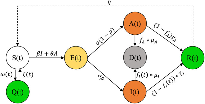
We present a model that accounts for social awareness measures, or their lack thereof, and asymptomatic infected individuals along with enhancements to compartmental models to capture the nonlinear trends of the COVID-19 epidemic curves that previous models did not fully realize [2]. These changes make our model capable of handling fluctuations in the susceptible compartment, allowing for more reliable model parameters determination. The present study borrows recent publications’ best features for a concise quarantine and asymptomatic aware SEIRD model. The Susceptible, Exposed, Asymptomatic, Infected, Recovered, Deceased, and Quarantined (SEAIRDQ) model is presented in Fig. 1 .
Fig. 1.
The proposed compartmental SEARIDQ model. The social awareness compartment, Q, contains individuals who are not susceptible (S), and will not be exposed (E). Individuals in the exposed compartment will either become asymptomatic infected (A), or symptomatic infected (I). The infected individuals (I or A) will subsequently either recover (R), or die (D, death compartment).
While adding multiple compartments [13,21,25,27,34] can help in proper allocation of available resources such as hospital beds or ventilators during this pandemic, the present study aims at developing a generalized model that can be used in similar epidemic conditions; as such, our model only uses the cumulative number of infected and dead individuals, along with the total population, as its inputs.
We assume that the pandemic's span is much shorter than the time needed for significant changes in the overall population to occur or for the natural ratio of death to birth to be affected. The social awareness compartment, Q, is defined as the individuals who are not susceptible (S), and will not be exposed (E) due to executive orders [21] that limit social presence at indoor/outdoor events, schools, or workplaces, or societal awareness factors including, but not limited to, the increased personal hygiene, social distancing, or wearing masks. It should be noted that our definition of the Q compartment is entirely different than the definition of [25] where infected individuals are quarantined at home after being positively tested.
The exposed compartment is subdivided into two sub-categories:
-
•
Symptomatic infected individuals (I)
-
•
Asymptomatic infected individuals (A)
Individuals in A do not have significant symptoms, are not tested positive, and are not hospitalized. In this compartment, an infected person may transmit the infection with a different rate , to the susceptible individuals since their symptoms (such as coughing or fever) are not as pronounced as the symptomatic infected individuals. Additionally, the course of their infection may be over with a rate other than the symptomatic individuals [21]. Equations (8)–(14) detail our model.
| (8) |
| (9) |
| (10) |
| (11) |
| (12) |
| (13) |
| (14) |
Table 1 lists the parameters used in the current model. Parameters β and θ are the infection rates in symptomatic and asymptomatic individuals, respectively. Similarly, and are the recovery rates of the symptomatic and asymptomatic individuals, respectively, with and being the rate of moving individuals from I and A to the recovered compartment, R. The time it takes for an infected individual to recover is determined through . Additionally, is taken to show what fraction of the asymptomatic individuals die and what fraction recover .
Table 1.
Modeling parameters used in the SEAIRDQ model and their respective definitions.
| Parameter | Description | Reported Value | Study Value |
|---|---|---|---|
| β | Infection rate of the symptomatic compartment | (1e-8,2e-6) | (0,0.5) |
| θ | Infection rate of the asymptomatic compartment | (1e-8,2e-6) | (0,0.5) |
| Fraction of the deceased infected individuals removed from I | |||
| Fraction of the deceased infected individuals removed from A | |||
| Recovery rate in the symptomatic compartment | (1/14,1/21) | (1/14,1/21) | |
| Recovery rate in the asymptomatic compartment | (1/14,1/21) | (1/14,1/21) | |
| Time that it takes for an infected individual in I to recover | |||
| Time that it takes for an infected individual in A to recover | |||
| σ | Incubation rate | (1/14,1/21) | (1/6,1/7.5) |
| Time that it takes for an exposed individual to show infection symptoms | |||
| ρ | Fraction of the exposed individuals ultimately becoming infected | ||
| ω | Effect of moving individuals from S to Q | ||
| ζ | Rate of leaving Q and becoming susceptible again | ||
| η | Rate of recovered individuals losing their immunity and returning to S |
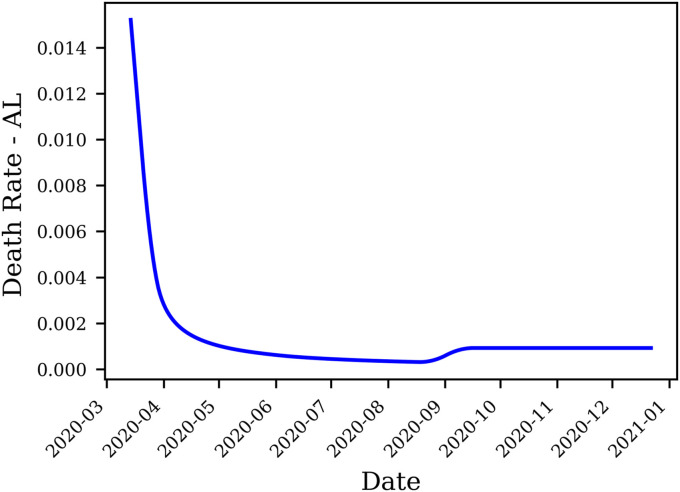
The death rate, denoted by μ, is not limited to the symptomatic compartment () only, as it can also occur in the asymptomatic compartment, denoted by . The vast improvements in medical knowledge and collaborative technology have made it possible to share the lessons learned in one country with other countries in no time; sharing findings and experiences translated to saving several lives. As a result, the death rate experienced in the early days of this pandemic was not the same as those observed later. For example, the death rate of the symptomatic individuals saw a considerable decrease, and taking it as a constant is no longer a valid assumption. The denominator in Equation (15) enables capturing different death rate trends in the symptomatic compartment, , whether it is increasing, constant, or decreasing.
| (15) |
Parameter σ shows the incubation rate, and shows the incubation time, i.e., the number of days it takes for an exposed individual to become infected. Parameter ρ signifies the fraction of exposed individuals that ultimately become infected (with for the symptomatic and for the asymptomatic compartments).
The shows the effect of moving individuals from S to Q, while accounts for the rate of leaving Q and becoming susceptible again. The and help in modeling the fluctuations of the susceptible compartment as the result of government orders, public awareness, and social distancing measures; in other words, shows the rate of reduction in S at each time-step. Unlike [34], we will not remove these individuals from S to add them to the recovered compartment (R), since they were neither exposed nor infected, to become immune in the future; instead, and are considered to be polynomial functions, allowing the model to handle nonlinear behavior of the epidemic curve.
| (16) |
| (17) |
In this model, η is considered the rate of recovered individuals losing their immunity against the virus and returning to the susceptible compartment. Parameter η can also be considered a factor that denotes the emergence of a mutated (and possibly more aggressive) variation of the virus, against which recovered individuals have no immunity.
The basic reproduction number, , is calculated based on the dominant eigenvalue of the NGM [11]:
| (18) |
As shown here, is dependent on β, which is governed by the population density, and which can be dictated by the health system infrastructure, hygiene, and availability of proper care. This signifies the uniqueness of and emphasizes the need for calculating it for each society, rather than borrowing it from one study area to another, as confirmed by Ref. [2].
Correct determination of the basic reproduction number allows for reliable calculation of another important epidemiological parameter, the herd immunity threshold . The represents the percentage of the population that needs to be protected against the infection to achieve herd immunity in the society [26], equation (19).
| (19) |
4. Methodology
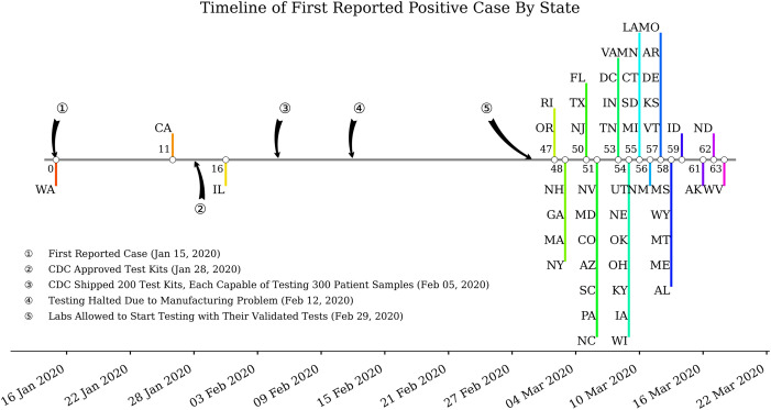
We conducted a comprehensive study of the COVID-19 pandemic at the national and regional levels; however, the early days of COVID-19 suffered from inadequate testing and lag in processing/reporting positive cases [10]. Based on the Centers for Disease Control and Prevention (CDC), the first case of the novel coronavirus was introduced to the US in Washington state on January 15, 2020, through travel from Wuhan, China [5]. Subsequent cases of infection were identified in California and Illinois on January 26 and January 31, respectively; however, for about a month until February 29, no additional cases were reported in other states across the US. Fig. 2 shows a timeline of the first reported cases across the US.
Fig. 2.
Timeline of first reported COVID-19 cases across the US. The large gap between early cases of COVID-19 reported in Washington and other states can be attributed to the availability of CDC-approved tests in other states.
During the early days of the COVID-19 pandemic, lack of appropriate testing meant that several positive cases went undetected until much later [29,31]. By the time more cases were identified in the US, different states had some level of early testing methods available to them, and detection of positive cases had become more reliable. As a result, a granular look at the spread of the virus at the state level can result in a more realistic determination of the basic reproduction number. Based on this observation, and since the determination of the basic reproduction number at the national level could introduce errors, authors used the mean basic reproduction number at the state level as the representative value for the US.
Initial conditions (ICs) play a critical role in the correct behavior of the ODEs. To set the most realistic ICs for the model, differential evolution was used on the first 60 days of the data (i.e., cumulative infections and deaths) in each state. The trained model is then used to estimate the correct ICs (, , , and ). These initial values are then used to perform a history match for the whole observation period and further refine the match parameters. The resulting models and fine-tuned parameters are later used to estimate the reproduction number, R, for each of the 50 states.
4.1. Data selection
By assuming that all individuals have an equal chance of being infected [22], we estimated the number of infected individuals and the mortalities in all states in the US. The number of daily death and reported confirmed infection cases were acquired at the county level for each state from Ref. [32]. According to Ref. [33], the data are pulled from the CDC, in addition to the state and local public health agencies. This data was combined with county-level metrics (including each county's population) to get an adequate measure of the virus's spread in each state. Aggregated county-level values were later used to model each state.
4.2. Model calibration
We adopted the approach of [34] for model calibration and to adjust our model parameters. Since common parameters such as recovery rates ( and ) and the incubation period (σ) are well studied in the literature, we aimed to calibrate the parameters that are not readily available in previous works (such as , , , , and ) or are unique to our presented model. We also included variables that are more sensitive to the output variable, i.e., β, θ, and ρ. This study uses the cumulative infected () and Death (D) as the observed quantities and defines a target output to fit these parameters.
4.3. Sensitivity analysis
To investigate how the model parameters sensitivity and some ICs affect specific modeled variables corresponding to observed input data, we used the Method of Morris (Elementary Effects method) [28] presented in the SALib library, an open-source Python library for sensitivity analysis [19], after [34].
The original Elementary Effects (EE) method presents two sensitivity measures for each input parameter: (i) the μ, evaluating the overall importance of an input parameter on the model output; (ii) the σ measure, defining non-linear effects and interactions. These two measures are obtained through a design based on the construction of a series of trajectories in the inputs’ space, where inputs are randomly moved one-at-a-time while others remain fixed. The region of experimentation omega is thus a k-dimensional p-level grid.
A specific parameter's first order sensitivity coefficient reveals how it is crucial to the target modeled variable. This study's sensitivity analysis evaluates all model parameters, , , , and to the target variable Y which is calculated using 20.
| (20) |
5. Results and discussion
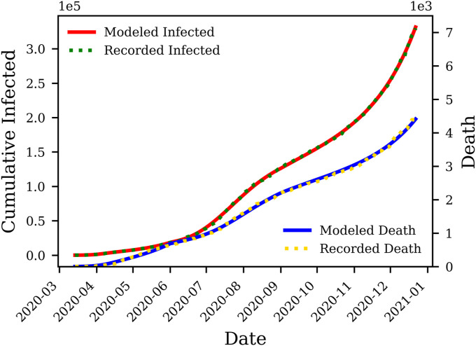
Exercising governmental orders and social awareness measures in different states has resulted in differences between initial and late spreading trends observed in the US. To capture these variabilities, the data were broken down at the inflection point intervals of approximately three months. Approaches used here have resulted in nearly perfect matches between the reported infections and deaths, versus the model outcomes. Co-visualizing cumulative death and infection cases on the same vertical axis can give false impressions about the match's accuracy for cumulative deaths. To avoid this problem, we present each one of the cumulative death and infection cases on a separate axis. As an example, Fig. 3 compares the output of the proposed model for cumulative infections and deaths in Alabama versus those observed in this state.
Fig. 3.
Deterministic history matching for death and cumulative symptomatic compartments in Alabama. The history match is performed for March 13, 2020 through December 22, 2020, with an accuracy of for matching the cumulative death, and for matching the cumulative infections.
5.1. Death rate
We can observe that the death rate exhibits a steady decline in most states; the death rate function for the state of Alabama, for example, is presented in Fig. 4 . The decrease in death rate can be attributed to better preparedness against the disease, which stems from understanding effective measures to increase the survival rate, including therapeutics’ availability.
Fig. 4.
Evolution of the death rate over time in Alabama estimated by the SEAIRDQ. A rolling average of 15 days window is applied. The death rate shows minute gain following the third peak in late August.
5.2. Symptomatic or asymptomatic
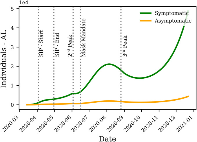
According to the laboratory data presented by Ref. [18], the asymptomatic individuals have a substantially greater number (up to 24 times) than estimated before, with the average SARS-CoV-2 positive infections being ten times more than the reported cases. To examine different theories surrounding the spread of the COVID-19 pandemic and validate their likelihood, we modeled different proportions of asymptomatic individuals, honoring both high and low ends of the possibility spectrum. In all of these cases, we aim to match the reported number of infections and deaths as accurately as possible. This is achieved through varying the death rates of I and A, as well as the size of the symptomatic and asymptomatic compartments.
Combining equations (11) and (12) shows that the ratio of asymptomatic to symptomatic compartments can be determined using ρ (the fraction of exposed individuals that ultimately become infected):
| (21) |
Based on equation (21), the model is allowed to place 13 times more individuals in the asymptomatic compartment compared to the symptomatic compartment, as (), paving the road to examine observations of [18]. A more conservative model with small sizes of the asymptomatic compartment is achieved when (). It is observed, however, that the average of ρ among all states is 0.749 (Table 2 ), suggesting that the asymptomatic population is about one third (1/3) of the symptomatic individuals. As an example, Fig. 5 shows a comparison between symptomatic and asymptomatic individuals in the state of Alabama.
Table 2.
The mean of SEAIRDQ modeling parameters after history matching the trend of COVID-19 disease in all 50 states in the US. The reported values reflect initial values that will be used by the model for subsequent runs.
| Parameter | Average |
|---|---|
| Death Rate | 0.0345 |
| Death Rate | 3.74e-04 |
| Recovery Rate | 0.0347 |
| Recovery Rate | 0.058 |
| 12.6 | |
| 90.0 | |
| 0.0604 | |
| 0.0583 | |
| 0.0949 | |
| 0.0697 | |
| 83.6 | |
| 0.407 | |
| 5.29e-03 | |
| ρ | 0.749 |
| β | 1.12e-05 |
| θ | 1.12e-05 |
| σ | 0.145 |
| 6.92 | |
| (days) | 17.1 |
| (days) | 17.7 |
| (days) | 13.9 |
| (days) | 15.3 |
Fig. 5.
The comparison between the symptomatic and asymptomatic infected individuals in the state of Alabama. The Shelter In Place (SIP) order was placed on April 3, 2020 and lifted on April 30, 2020. The peak of infection, observed in early June, is followed by a mask mandate in mid-June. A slow down is observed until the peak in late August, which coincides with the reopening of schools.
It should be noted that models with high ratios of asymptomatic patients are still possible for early portions of the data; however, such models fail to match the extended history of the disease's progression in each state. As a result, the average one-third ratio of asymptomatic to symptomatic infections observed in this study is due to the longer time span covered by the present work, compared to the early days of the pandemic where testing was not readily available; thus, observations of [18] cannot be verified through our modeling.
5.3. Initial susceptible population
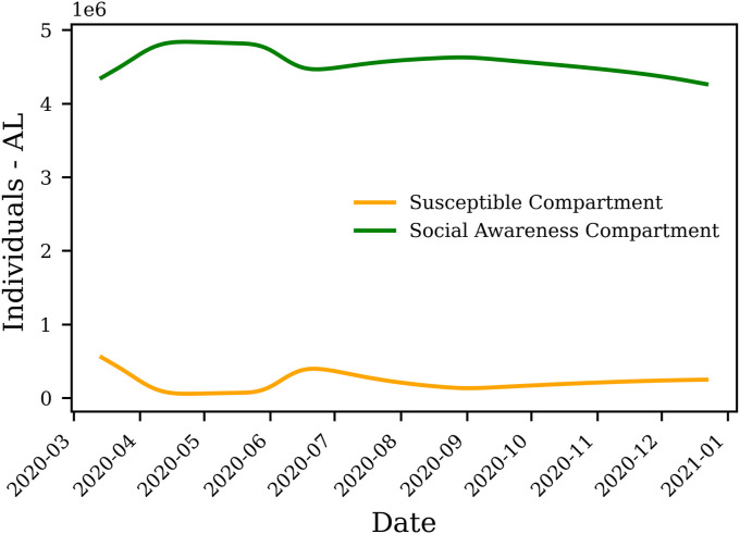
One of the most critical parameters affecting compartmental modeling is the initial susceptible population, . What makes the COVID-19 pandemic unique is the abundance of information and public awareness about this virus. The first infections in many communities were encountered while a significant portion of the population was already on high alert and practiced self-isolation long before; thus, the initial population of the (social awareness and quarantine compartment), which reflects non-susceptible individuals, is considerably high.
Precluding a reasonable , i.e., results in , where N is the total population. It should be noted that the majority of the compartmental models, except for [7,21], take to be the same as N. However, the ensemble results of our study show that the mean in the US is . Forcing to a small value, for example, 0 necessitates a rapid increase in Q (for one day) for the model to match the trends of cumulative symptomatic infections and deaths. Fig. 7 shows the evolution of Q and S compartments in the state of Alabama.
Fig. 7.
Modeled Q and S compartment for Alabama. Fluctuations in the number of individuals in the social awareness compartment (Q) reflects instigation of state-wide orders and individuals adhering to social awareness measures. These fluctuations in Q result in alteration of the number of susceptible individuals (S) over time.
5.4. Initial basic reproduction number
Table 2 shows the average observations made for the US. According to Table 2, the average of is determined to be 12.6, with the average incubation time in the US estimated to be 6.92 days. As an example, Fig. 8 shows the trend of reproduction number in the state of Alabama. While an of this magnitude can seem extremely high and raise many questions regarding the validity of observations, it is noteworthy that Jia [21] also reported the in different ranges (e.g., 8.5 for inside and 12.7 for outside of Hubei), far greater than the 2.2 reported by Ref. [24].
Fig. 8.
Trend of the reproduction number (R) over time in the state of Alabama. A decrease in R is observed as the Shelter In Place (SIP) order was instigated on April 3, 2020 and lifted on April 30, 2020. R picks up again in early June following the peak in the state. The Mask mandate of mid-June slowed down the spread and R. The reproduction number picked up again following the of late August.
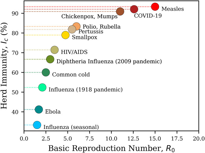
An of 12.6 puts COVID-19 among the most contagious infections, such as Mumps, Chickenpox, or Measles [17]. Fig. 6 shows a comparison between the basic reproduction number of the current COVID-19 pandemic with previously contagious diseases. The average of herd immunity for the aforementioned conditions in the US is found to be .
Fig. 6.
The comparison between the basic reproduction number () of different contagious diseases, with their corresponding herd immunity percentages, modified after [16]. Our estimated average of 12.6 in the US, puts COVID-19 among the most contagious infections, such as Mumps, Chickenpox, or Measles [17].
5.5. Model calibration and sensitivity analysis
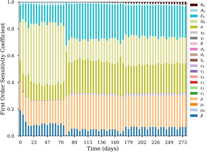
The first order sensitivity coefficient results suggest that uncertainties on and β can induce significant changes in the early epidemic trend during executive orders. However, the impact of such uncertainties decreases as the epidemic evolves, indicating that other parameters such as , ρ, and σ have more influence in the long term. The most important parameter is the , and its impact decreases after the relaxing some executive orders. (Fig. 10 ).
Fig. 10.
First-order sensitivity coefficient of all model parameters over time for Alabama.
5.6. Forecasting
Governmental decisions, the general population's response, and mass vaccination scenarios will result in different epidemic trends. Several studies have aimed to predict the number of deaths and confirmed cases related to COVID-19 [7,14,21,27,34,35,39], along with a possible end date for the pandemic or transition into an endemic [30]. Our proposed model can use the parameters extracted from the most recent 90 days of data to forecast the future. While such modeling and forecasting approaches are needed, our goal was to introduce a model capable of handling the non-linear trend and dissect its fundamental behavior (such as basic and effective reproduction numbers) through accurate history matching. Examining different societal scenarios and vaccine effectiveness requires another dedicated study and falls outside the scope of the present work.
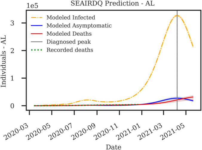
Table 3 shows a detailed comparison between estimated modeling results and the recorded cases for the state of Alabama from March 13, 2020, through December 22, 2020. As demonstrated in Table 3, and Fig. 3, the present model has an accuracy of more than for matching death and over for cumulative infections. To examine the outcome of this model for the state of Alabama, the most recent recorded confirmed cases available as of this writing were acquired, and a forecasting period of 200 days was selected. We used the fitting parameters from the third portion of the data (September 1, 2020 through December 22, 2020) for this forecasting. Fig. 9 shows the forecast of the pandemic in Alabama until July 2021. Assuming that the current trends continue onward, it is anticipated that the next major wave of the disease in the state of Alabama will hit towards the end of April, with magnitudes far more significant than what the state has already seen.
Table 3.
Comparison between the recorded cases, and the outcome of the SEAIRDQ model for the state of Alabama through December 22, 2020.
| Parameter | Value |
|---|---|
| Total population | 4,903,185 |
| Deaths (Recorded) | 4452 |
| Deaths (Estimated - SEAIRDQ) | 4400 |
| Estimated Death Accuracy | 98.83% |
| Estimated Death Percentage of the Population (SEAIRDQ) | 0.090% |
| Confirmed cases | 329,811 |
| Confirmed cases (Estimated - SEAIRDQ) | 331,808 |
| Estimated Confirmed Cases Accuracy | 99.39% |
| Estimated Infected Percentage of the Population (SEAIRDQ) | 6.767% |
| Estimated Starting Date of the Second Peak | First Week of Jun |
| Estimated Starting Date of Third Peak | Last Week of August |
Fig. 9.
Probabilistic SEAIRDQ forecast of the COVID-19 pandemic in the state of Alabama through July 2021. It is anticipated that the significant wave of infections in the state will start towards the end of April 2021.
6. Conclusion
This paper presented a new compartmental model capable of capturing the non-linear behavior of the COVID-19 pandemic while accounting for asymptomatic infected individuals. Fluctuations in the susceptible individuals (S), due to social awareness and governmental orders, were modeled through the introduction of a social awareness compartment (Q), where a set of polynomial functions controlled the movement of individuals between S and Q. The present study fitted the observed cumulative infected individuals and cumulative deaths reported in each state with an accuracy of for matching the cumulative deaths and for matching the cumulative infections. We presented an ensemble of results for the spread of the virus in the US, along with detailed results for Alabama. While minute fluctuations were observed over time, we found the average ratio of asymptomatic infected individuals to be about one-third of the symptomatic infected individuals. We also found the average reproduction number of COVID-19 to be 12.6 across the US, putting this virus among the most contagious infections, such as Mumps and Measles. Additionally, the average herd immunity in the US was estimated to be . The presented methodology, along with its results and observations can pave the road to better evaluation of different strategies at the federal and state levels.
Declaration of competing interest
None Declared.
Biographies

Somayeh Bakhtiari Ramezani is a Ph.D. Candidate at the Computer Science and Engineering Department, Mississippi State University, with research interests spanning compartmental modeling, optimization, machine learning, quantum computation, and time-series segmentation.

Amin Amirlatifi is an Assistant Professor of chemical and petroleum engineering at Swalm School of Chemical Engineering, Mississippi State University. His research interests include numerical modeling, artificial intelligence, and predictive maintenance.

Shahram Rahimi is professor and department head of the Computer Science and Engineering Department at the Mississippi State University. His research interests include Computational Intelligence, Soft Computing and Machine Learning, and Predictive Analytics with Game Theory.
References
- 1.Anderson R.M., May R.M. first ed. Oxford University Press; London: 1992. Infectious Diseases in Humans. [Google Scholar]
- 2.Anderson R.M., Vegari C., Baggaley R., Hollingsworth T.D., Maddren R. The Royal Society; 2020. Reproduction Number (R) and Growth Rate (R) of the COVID-19 Epidemic in the UK: Methods of Estimation, Data Sources, Causes of Heterogeneity, and Use as a Guide in Policy Formulation. [Google Scholar]
- 3.Bernoulli D. Essai d’une nouvelle analyse de la mortalité causée par la petite vérole, et des avantages de l’inoculation pour la prévenir. Histoire de l’Acad., Roy. Sci.(Paris) avec Mem. 1760:1–45. [Google Scholar]
- 4.Britton T., Ball F., Trapman P. A mathematical model reveals the influence of population heterogeneity on herd immunity to SARS-CoV-2. Science. 2020;369:846–849. doi: 10.1126/science.abc6810. [DOI] [PMC free article] [PubMed] [Google Scholar]
- 5.CDC First travel-related case of 2019 novel coronavirus detected in United States. 2020. https://www.cdc.gov/media/releases/2020/p0121-novel-coronavirus-travel-case.html URL.
- 6.Chang S.L., Piraveenan M., Prokopenko M. The effects of imitation dynamics on vaccination behaviours in SIR-network model. Int. J. Environ. Res. Publ. Health. 2019;16:2477. doi: 10.3390/ijerph16142477. https://www.mdpi.com/1660-4601/16/14/2477 URL. [DOI] [PMC free article] [PubMed] [Google Scholar]
- 7.Chatterjee S., Sarkar A., Chatterjee S., Karmakar M., Paul R. Studying the progress of COVID-19 outbreak in India using SIRD model. Indian J. Phys. 2020:1–17. doi: 10.1007/s12648-020-01766-8. https://link.springer.com/article/10.1007/s12648-020-01766-8 [DOI] [PMC free article] [PubMed] [Google Scholar]
- 8.Chowell G., Hengartner N.W., Castillo-Chavez C., Fenimore P.W., Hyman J.M. The basic reproductive number of Ebola and the effects of public health measures: the cases of Congo and Uganda. J. Theor. Biol. 2004;229:119–126. doi: 10.1016/j.jtbi.2004.03.006. [DOI] [PubMed] [Google Scholar]
- 9.Culp W.C. Coronavirus disease 2019. A & A Practice. 2020;14 doi: 10.1213/xaa.0000000000001218. [DOI] [PMC free article] [PubMed] [Google Scholar]
- 10.Davis K. Better late than never: COVID-19 testing across the United States. 2020. https://sitn.hms.harvard.edu/flash/2020/covid-19-testing/ URL.
- 11.Diekmann O., Heesterbeek J.A., Roberts M.G. The construction of next-generation matrices for compartmental epidemic models. J. R. Soc. Interface. 2010;7:873–885. doi: 10.1098/rsif.2009.0386. [DOI] [PMC free article] [PubMed] [Google Scholar]
- 12.Du Z., Xu X., Wu Y., Wang L., Cowling B.J., Meyers L.A. Serial interval of COVID-19 among publicly reported confirmed cases. Emerg. Infect. Dis. 2020;26:1–7. doi: 10.3201/eid2606.200357. [DOI] [PMC free article] [PubMed] [Google Scholar]
- 13.Duque D. 2020. COVID-19 How to Relax Social Distancing if You Must.http://medrxiv.org/cgi/content/short/2020.04.29.20085134 Medrxiv URL. [Google Scholar]
- 14.Duque D., Morton D.P., Singh B., Du Z., Pasco R. 2020. COVID-19 in Austin , Texas : Averting Healthcare Surges while Relaxing Social Distancing COVID-19 in Austin , Texas : Averting Healthcare Surges while Relaxing Social Distancing. Technical Report. The University of Texas at Austin, COVID-19 Modeling Consortium. Austin.https://sites.cns.utexas.edu/sites/default/files/cid/files/austin_covid-19_optimized_relaxation_of_social_distancing_0428020.pdf?m=1588082043 URL. [Google Scholar]
- 15.Fernández-Villaverde J., Jones C. National Bureau of Economic Research; Cambridge, MA: 2020. Estimating and Simulating a SIRD Model of COVID-19 for Many Countries, States, and Cities. Technical Report.http://www.nber.org/papers/w27128.pdf URL. [DOI] [PMC free article] [PubMed] [Google Scholar]
- 16.Fine P., Eames K., Heymann D.L. Herd immunity and implications for SARS-CoV-2 control. Clin. Infect. Dis. 2020;52:911–916. doi: 10.1093/cid/cir007. [DOI] [PubMed] [Google Scholar]
- 17.Guerra F.M., Bolotin S., Lim G., Heffernan J., Deeks S.L., Li Y., Crowcroft N.S. The basic reproduction number (R 0) of measles: a systematic review. Lancet Infect. Dis. 2017;17:e420–e428. doi: 10.1016/S1473-3099(17)30307-9. https://linkinghub.elsevier.com/retrieve/pii/S1473309917303079 URL. [DOI] [PubMed] [Google Scholar]
- 18.Havers F.P., Reed C., Lim T., Montgomery J.M., Klena J.D., Hall A.J., Fry A.M., Cannon D.L., Chiang C.F., Gibbons A., Krapiunaya I., Morales-Betoulle M., Roguski K., Rasheed M.A.U., Freeman B., Lester S., Mills L., Carroll D.S., Owen S.M., Johnson J.A., Semenova V., Blackmore C., Blog D., Chai S.J., Dunn A., Hand J., Jain S., Lindquist S., Lynfield R., Pritchard S., Sokol T., Sosa L., Turabelidze G., Watkins S.M., Wiesman J., Williams R.W., Yendell S., Schiffer J., Thornburg N.J. Seroprevalence of antibodies to SARS-CoV-2 in 10 sites in the United States, March 23-may 12, 2020. JAMA Inter. Med. 2020;180:1776–1786. doi: 10.1001/jamainternmed.2020.4130. https://jamanetwork.com/journals/jamainternalmedicine/fullarticle/2768834 URL. [DOI] [PMC free article] [PubMed] [Google Scholar]
- 19.Herman J., Usher W. SALib: an open-source Python library for Sensitivity Analysis. J. Open Sour. Softw. 2017;2:97. doi: 10.21105/joss.00097. [DOI] [Google Scholar]
- 20.Javan E., Fox S.J., Meyers L.A. Probability of current COVID-19 outbreaks in all US counties. medRxiv. 2020 doi: 10.1101/2020.04.06.20053561. http://medrxiv.org/content/early/2020/04/11/2020.04.06.20053561.abstract [DOI] [Google Scholar]
- 21.Jia J., Ding J., Liu S., Liao G., Li J., Duan B.E., Wang G., Zhang R.A. Modeling the control of COVID-19: impact of policy interventions and meteorological factors. Electron. J. Differ. Equ. 2020:1–24. [Google Scholar]
- 22.Kermack W.O., McKendrick A.G. vol. 115. 1927. A contribution to the mathematical theory of epidemics; pp. 700–721.https://royalsocietypublishing.org/doi/10.1098/rspa.1927.0118 (Proceedings of the Royal Society of London. Series A, Containing Papers of a Mathematical and Physical Character). URL. [Google Scholar]
- 23.Kermack W.O., McKendrick A.G. Contributions to the mathematical theory of epidemics-II.-The Problem of Endemicity. Bull. Math. Biol. 1932;53:55–83. doi: 10.1007/BF02464423. [DOI] [PubMed] [Google Scholar]
- 24.Li Q., Guan X., Wu P., Wang X., Zhou L., Tong Y., Ren R., Leung K.S., Lau E.H., Wong J.Y., Xing X., Xiang N., Wu Y., Li C., Chen Q., Li D., Liu T., Zhao J., Liu M., Tu W., Chen C., Jin L., Yang R., Wang Q., Zhou S., Wang R., Liu H., Luo Y., Liu Y., Shao G., Li H., Tao Z., Yang Y., Deng Z., Liu B., Ma Z., Zhang Y., Shi G., Lam T.T., Wu J.T., Gao G.F., Cowling B.J., Yang B., Leung G.M., Feng Z. Early transmission dynamics in wuhan, China, of novel coronavirus–infected pneumonia. N. Engl. J. Med. 2020;382:1199–1207. doi: 10.1056/nejmoa2001316. [DOI] [PMC free article] [PubMed] [Google Scholar]
- 25.Lingzhi M., Bouardi H.T., Lami O.S., Trichakis N., Trikalinos T., Zarandi M.F., Bertsimas D. MassachusettsInstituteofTechnology; 2020. Overview of DELPHI Model. Technical Report April. [Google Scholar]
- 26.Masterson S.G., Lobel L., Carroll M.W., Wass M.N., Michaelis M. Herd immunity to Ebolaviruses is not a realistic target for current vaccination strategies. Front. Immunol. 2018;9:1–7. doi: 10.3389/fimmu.2018.01025. [DOI] [PMC free article] [PubMed] [Google Scholar]
- 27.Moghadas S.M., Shoukat A., Fitzpatrick M.C., Wells C.R., Sah P., Pandey A., Sachs J.D., Wang Z., Meyers L.A., Singer B.H., Galvani A.P. Projecting hospital utilization during the COVID-19 outbreaks in the United States. Proc. Natl. Acad. Sci. U.S.A. 2020;117:9122–9126. doi: 10.1073/pnas.2004064117. [DOI] [PMC free article] [PubMed] [Google Scholar]
- 28.Morris M.D. Factorial sampling plans for preliminary computational experiments. Technometrics. 1991;33:161–174. doi: 10.1080/00401706.1991.10484804. [DOI] [Google Scholar]
- 29.Rivero E. 2020. COVID-19 May Have Been in L.A. As Early as Last December, UCLA-led Study Suggests — UCLA.https://newsroom.ucla.edu/releases/covid-may-have-been-in-la-as-early-as-december-2019 URL. [Google Scholar]
- 30.Shaman J., Galanti M. Will SARS- CoV-2 become endemic? Science. 2020;370:527–530. doi: 10.1126/science.abe5960. [DOI] [PubMed] [Google Scholar]
- 31.St John P., Mason M., Hamilton M. California coronavirus spread began earlier than reported - los Angeles Times. 2020. https://www.latimes.com/california/story/2020-04-23/morgues-hold-key-to-early-spread-of-coronavirus URL.
- 32.USA Facts, 2020. USA Facts - US Coronavirus Cases and Deaths. https://usafactsstatic.blob.core.windows.net/public/data/covid-19/covid_confirmed_usafacts.csvhttps://usafactsstatic.blob.core.windows.net/public/data/covid-19/covid_confirmed_usafacts.csvhttps://usafactsstatic.blob.core.windows.net/public/data/covid-19/covid_deaths_usafacts.csv URL.
- 33.USAFacts Detailed methodology and sources: COVID-19 data. 2020. https://usafacts.org/articles/detailed-methodology-covid-19-data/ URL.
- 34.Volpatto D., Resende A.C., dos Anjos L., Silva J., Dias C., Almeida R., Malta S. Spreading of COVID-19 in Brazil: impacts and uncertainties in social distancing strategies. medRxiv. 2020 doi: 10.1101/2020.05.30.20117283. [DOI] [Google Scholar]
- 35.Wang X., Du Z., Huang G., Fox S., Meyers L.A. The University of Texas at Austin; 2020. COVID-19 in Austin , Texas : Relaxing Social Distancing Measures COVID-19 in Austin , Texas : Relaxing Social Distancing Measures. Technical Report.https://sites.cns.utexas.edu/sites/default/files/cid/files/austin_relaxing_social_distancing.pdf?m=1587681780 COVID-19 Modeling Consortium. Austin, TX. URL. [Google Scholar]
- 36.Wang X., Du Z., Pasco R., Pierce K., Petty M., Fox S.J., Pignone M., Johnston C., Meyers L.A. The University of Texas at Austin; Austin: 2020. COVID-19 Healthcare Demand Projections: Austin, Texas. Technical Report. [Google Scholar]
- 37.Wang X., Pasco R.F., Du Z., Petty M., Fox S.J., Galvani A.P., Pignone M., Johnston S.C., Meyers L.A. Impact of social distancing measures on COVID-19 healthcare demand in central Texas. medRxiv. 2020 doi: 10.1101/2020.04.16.20068403. http://medrxiv.org/content/early/2020/04/22/2020.04.16.20068403.abstract [DOI] [PMC free article] [PubMed] [Google Scholar]
- 38.Weitz J.S., Dushoff J. Modeling post-death transmission of Ebola: challenges for inference and opportunities for control. Sci. Rep. 2015;5:1–7. doi: 10.1038/srep08751. [DOI] [PMC free article] [PubMed] [Google Scholar]
- 39.Woody S., Garcia Tec M., Dahan M., Gaither K., Fox S., Meyers L.A., Scott J.G. Projections for first-wave COVID-19 deaths across the US using social-distancing measures derived from mobile phones. medRxiv. 2020 doi: 10.1101/2020.04.16.20068163. http://medrxiv.org/content/early/2020/04/22/2020.04.16.20068163.abstract [DOI] [Google Scholar]
- 40.World Health Organization Naming the coronavirus disease (COVID-19) and the virus that causes it. https://www.who.int/emergencies/diseases/novel-coronavirus-2019/technical-guidance/naming-the-coronavirus-disease-(covid-2019)-and-the-virus-that-causes-it URL.
- 41.Zhang H., Yingqi L., Xu W. Global stability of an SEIS epidemic model with general saturation incidence. ISRN Appl. Math. 2013:1–11. doi: 10.1155/2013/710643. [DOI] [Google Scholar]
- 42.Zou D., Wang L., Xu P., Chen J., Zhang W., Gu Q. Epidemic model guided machine learning for COVID-19 forecasts in the United States. medRxiv. 2020 doi: 10.1101/2020.05.24.20111989. [DOI] [Google Scholar]


