A map of object space in primate inferotemporal cortex

Abstract

The inferotemporal (IT) cortex is responsible for object recognition, but it is unclear how the representation of visual objects is organized in this part of the brain. Areas that are selective for categories such as faces, bodies, and scenes have been found^1–5, but large parts of IT cortex lack any known specialization, raising the question of what general principle governs IT organization. Here we used functional MRI, microstimulation, electrophysiology, and deep networks to investigate the organization of macaque IT cortex. We built a low-dimensional object space to describe general objects using a feed forward deep neural network trained on object classification⁶. Responses of IT cells to a large set of objects revealed that single IT cells project incoming objects onto specific axes of this space. Anatomically, cells were clustered into four networks according to the first two components of their preferred axes, forming a map of object space. This map was repeated across three hierarchical stages of increasing view invariance, and cells that comprised these maps collectively harboured sufficient coding capacity to approximately reconstruct objects. These results provide a unified picture of IT organization in which category-selective regions are part of a coarse map of object space whose dimensions can be extracted from a deep network.

Object recognition, the process by which distinct visual forms are assigned distinct identity labels, lies at the heart of our ability to make sense of the visual world. It underlies many neural processes that operate on objects, including consciousness, attention, visual memory, decision making, and language. Befitting the central importance and computational complexity of object recognition, a large volume of the brain, IT cortex, is dedicated to solving this challenge⁷.

One of the most striking features of IT is the existence of several distinct anatomical networks that are specialized for processing specific categories^2,4,5 or stimulus dimensions^8–11. However, these networks comprise only part of IT, and much of IT is not differentially activated by any known stimulus comparison. Here we investigate whether this ‘unexplained’ IT shows any functional specialization. Furthermore, beyond simply parcelling IT, we investigate whether there is an overarching general principle governing the anatomical layout of IT cortex.

Many previous studies have tried to address this latter question, but the answers obtained remain piecemeal. Early studies using electrophysiology in monkeys suggested a columnar architecture for visual shape¹², but the small field-of-view of electrophysiology precluded understanding the larger-scale organization of these columns. Later studies, using functional MRI (fMRI) in humans, proposed various schemes to explain large-scale IT organization including retinotopy¹³ and real-world size¹⁴, but these proposals did not provide a complete account of IT organization and lacked ground-truth validation at the level of single units. Here, we combined fMRI, electrical microstimulation, and electrophysiology in the same animals to investigate the organization of macaque IT at multiple scales, and found that a large portion of macaque IT cortex is topographically organized into a map of object space that is repeated three times.

Identifying a new IT network

To discover the functional specialization of still unexplained parts of IT cortex, one strategy would be to guess. However, lacking any good guesses, we decided to approach the problem from an anatomical perspective. We ran a large set of stimulus comparisons to localize face, body, scene, colour, and disparity patches in a specific monkey (Ml) and thereby define the ‘no man’s land’ of IT cortex in this monkey: regions that were not identified by any known localizer (Fig. 1a, b). We then electrically microstimulated a random site within this no man’s land in central IT cortex¹⁵. This experiment revealed that the stimulated region (NML2) was connected to two other, discrete regions in IT (NML1, NML3) (Fig. 1b, Extended Data Fig. 1), forming a previously unknown anatomical network within no man’s land.

Fig. 1: Microstimulation reveals a new anatomical network in IT cortex.

a, Stimulus contrasts used to identify known networks in IT (see Methods), b, Inflated brain (right hemisphere) for monkey M1 showing known IT networks mapped in this animal. Regions activated by microstimulation of NML2 are shown in yellow. All activation maps shown at a threshold of P < 10⁻³ not corrected for multiple comparisons. Yellow and magenta outlines indicate the boundaries of TE and TEO, respectively³⁹.

To understand the function of this new network, we first recorded the neural responses of cells in the three patches to 1,224 images, consisting of 51 objects each presented at 24 views belonging to 6 different categories (Extended Data Fig. 2a, b). Responses were remarkably consistent (Fig. 2a, Extended Data Fig. 3a–d). Cells in all three patches responded minimally to faces. Their preferred stimuli, while consistent across patches, were not confined to any one semantic category (Fig. 2a).

Fig. 2: Distinct object preferences among four different networks in IT cortex.

a–d, Top, responses of cells to 51 objects from six different categories. Responses to each object were averaged across 24 views. Cells were recorded in three patches (NML1, NML2 and NML3) from the NML network (a); in three patches of the body network (b); in patch ML of the face network (c); and in two patches of the stubby network (d). Middle, blue charts show average responses to each object in each network. Numbers indicate the five most-preferred objects. Bottom, five most-preferred (top row) and least-preferred (bottom row) objects for each network, based on averaged responses; images 1 to 5 are shown from left to right, e, Coronal slices containing NML1, NML2, and NML3 from monkeys M1, M2, M3, and M4 showing difference in activation in response to the five most-preferred versus five least-preferred objects determined from electrophysiology in the NML network of monkey M1. In M1, the microsimulation result is also shown as a cyan overlay with threshold P < 10⁻³, uncorrected. Inset numbers indicate AP coordinate relative to interaural 031. f, Responses of cells from patches NML2 and NML3 of the NML network to a line segment that varied in aspect ratio, curvature, and orientation. Responses are averaged across orientation, and curvature runs from low to high from left to right for each aspect ratio. Aspect ratio accounts for 22.8% of response variance on average across cells, curvature for 5.6% of variance, and orientation for 3.5% of variance.

To investigate whether this network exists in every animal, we identified the five most- and least-preferred objects of the network based on mean responses of cells recorded from monkey M1 (Fig. 2a). We presented these stimuli to monkey M1 in an fMRI experiment and confirmed that the resulting map overlapped that revealed by microstimulation (Fig. 2e). We then presented these stimuli to three other monkeys (M2–M4) and found similar networks in all three animals (Fig. 2e). Single-unit recordings targeted to this network in monkey M2 revealed a response pattern that was highly consistent with that in monkey M1 (Fig. 2a) (Pearson correlation of the mean responses to each object between monkeys M1 and M2, r = 0.89, P < 10⁻¹⁶). This justifies referring to an ‘NML network’ across animals.

In the face patch network, neurons in posterior patches are view-specific whereas those in the most anterior patch are view-invariant¹⁶. We found a similar difference between the three NML patches in terms of their view invariance. Significantly more cells in NML3 were view-invariant than in NML1 (two-tailed t-test; t(137) = 5.10, P < 10⁻⁵; Extended Data Fig. 3e). Population similarity matrices to objects at different views also showed an increase in view invariance going anteriorly, with emergence of parallel diagonal stripes in the NML3 similarity matrix (Fig. 3a (top), Extended Data Fig. 3f). Notably, many cells showed view invariance to objects that the monkey had not experienced, such as an aeroplane (Fig. 3b (top)).

Fig. 3: Each network contains a hierarchy of increasingly view-invariant nodes, and single cells in each node show ramp-shaped tuning.

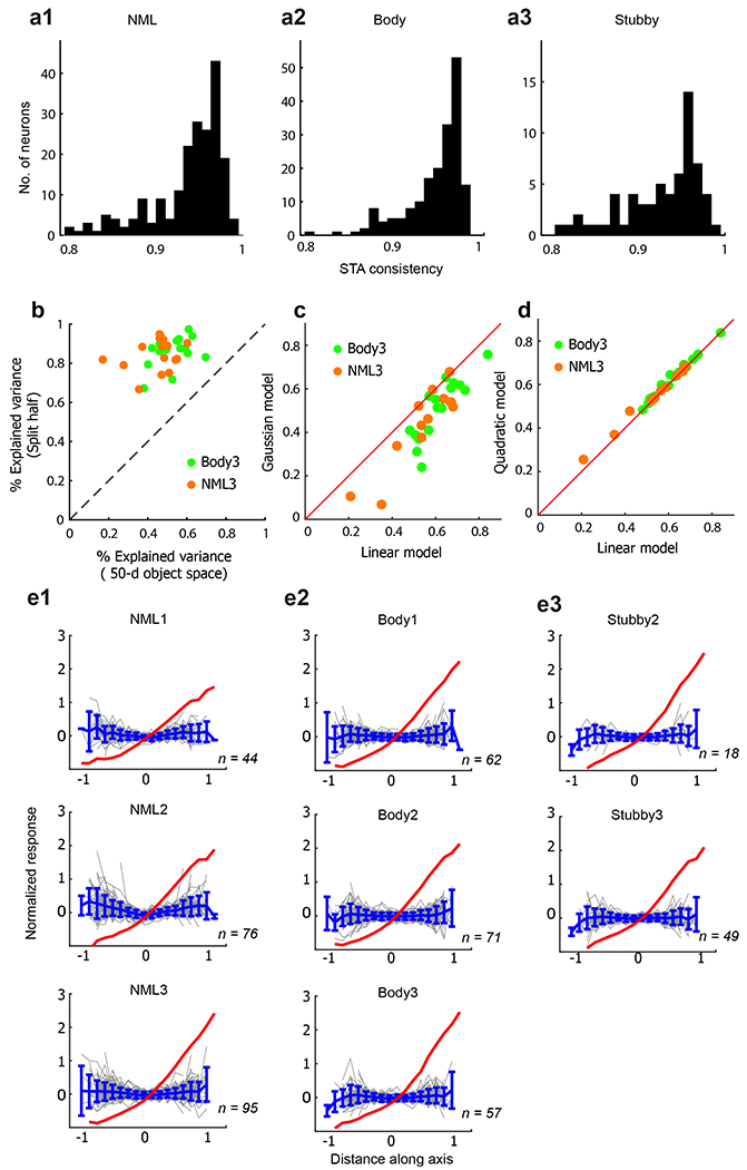
a, Population similarity matrices in the three patches of the NML network (top), three patches of the body network (middle) and two patches of the stubby network (bottom) pooled across monkeys M1 and M2. An 88 × 88 matrix of correlation coefficients was computed from responses of cells in each patch to 88 stimuli (8 views × top 11 preferred objects). b, Responses from three example cells recorded in NML3 (top), the body network (middle) and the stubby network (bottom) to 51 objects at 24 views. Four different views of the most preferred object are shown below each response matrix. c, Responses of neurons recorded from patches in the NML network (top), the body network (middle) and the stubby network (bottom) as a function of distance along the preferred axis. The abscissa is rescaled so that the range [−1,1] covers 95% of the stimuli. Half the stimulus trials were used to compute the preferred axis for each cell, and held-out data were used to plot the responses shown.

Next, we investigated what is being coded by cells in this network. Scrutinizing the most- and least-preferred objects (Fig. 2a (bottom)), we noticed that all of the preferred objects contained thin protrusions, whereas the non-preferred objects were round. This suggested that one feature NMF neurons might be selective for is high aspect ratio. We confirmed this using both responses to the original object image set (Extended Data Fig. 3g, see Methods) as well as a simplified stimulus set consisting of a line segment independently varied in aspect ratio, curvature, and orientation (Fig. 2f, Extended Data Fig. 2c). Thus a common preferred feature of cells in the NMF network is high aspect ratio.

NML cells encode axes of object space

We next attempted to identify the relevant shape dimensions for the NMF network in a systematic way that does not depend on subjective visual inspection. Until recently, this was difficult because of the lack of a computational scheme to parametrize arbitrary objects. Deep networks trained to classify objects provide a powerful solution to this problem¹⁷. They allow parametrization of arbitrary objects through computation of a few thousand numbers, the unit activations in a deep layer. To make the parametrization even more compact, one can perform principal components analysis (PCA) on these unit activations.

We built an object space by passing the stimulus set we presented to the monkey (Extended Data Fig. 2a, b) through AlexNet, a deep network trained on object classification6, and then performing PCA on the responses of units in layer fc6 of this network (Extended Data Fig. 4a). The first principal component (PC) corresponds roughly to things with protrusions (spiky) versus those without (stubby) (Extended Data Fig. 4b). The second PC corresponds roughly to animate versus inanimate (note that we use ‘animate’ and ‘inanimate’ as shape descriptors without any semantic connotation). We determined that 50 object dimensions could explain 85% variance in the AlexNet fc6 response (Extended Data Fig. 4c) and thus used 50 dimensions in the remaining analyses. We then analysed the responses of cells in the NML network by computing a ‘preferred axis’ for each cell through linear regression, namely, the coefficients c in the equation R = c·f + c₀, where R is the response of the cell, f is the 50D object feature vector, and c₀ is a constant offset (see Methods).

Cells showed significant tuning to many of the 50 object dimensions (Pearson correlation P < 10⁻³ between feature values and neural responses). On average, each cell was significantly tuned to seven dimensions. Notably, the preferred axis of each cell was stable to the precise image set (Extended Data Fig. 5a). The 50D linear object space model could explain 44.7% variance, or 53.3% of the explainable variance of NML neurons on average (Extended Data Fig. 5b); this is significantly higher than a Gaussian model and similar to a quadratic model (Extended Data Fig. 5c, d). Consistent with the high explained variance by the linear model, cell tuning along the preferred axis in the 50D object space was ramp-shaped (Fig. 3c, top). Similar ramp-shaped tuning has previously been reported for face-selective cells¹⁸. NML neurons also showed approximately flat tuning along orthogonal axes (Extended Data Fig. 5e), another property that has been previously observed in face-selective cells¹⁸. Together, ramp-shaped tuning along the preferred axis and flat tuning along orthogonal axes implies that cells in the NML network are linearly projecting incoming objects, formatted as vectors in object space, onto specific preferred axes.

Overall, the organization and code of the NML network are strikingly similar to those of the face patch network. The NML network consists of connected patches, cells within the network show a consistent pattern of selectivity, there is increasing view invariance along the network, and finally, single cells in the network represent object identity through an axis code. Thus there seems to be a clear structural parallel between the face network and the NML network. We therefore investigated whether additional networks in IT cortex follow the same scheme.

The body network follows the same scheme

We next recorded from the macaque body network, a set of regions adjacent to face patches that respond more to animate compared to inanimate objects⁴ (Fig. 2b), as well as the face network (Fig. 2c). Population similarity matrices showed increased view invariance in the most anterior body patch (Fig. 3a, b (middle), Extended Data Fig. 3e, f), consistent with a previous study¹⁹. Cells in the body network also showed ramp-shaped tuning along their preferred axes (Fig. 3c (middle), Extended Data Fig. 5a) and flat tuning along orthogonal axes (Extended Data Fig. 5e). Thus the body network follows the same general anatomical organization and coding scheme as the NML and face networks.

A general rule governing IT organization

The finding of three networks (NML, body and face) that all follow the same organization and coding scheme suggests that there might be a general principle that governs the organization of IT cortex. Recall that the first two axes of object space are roughly stubby versus spiky, and animate versus inanimate (Extended Data Fig. 4b). We noticed a remarkable relationship between these two axes and the selectivity of the NML, body, and face networks. Face patches prefer stubby animate objects; body patches prefer spiky, animate objects; and NML patches prefer spiky objects regardless of animacy (Fig. 2a). These observations made us wonder whether all of IT might be topographically organized according to the first two dimensions of object space (Fig. 4a), in the same way that retinotopic cortex is organized according to polar angle and eccentricity.

Fig. 4: A map of object space revealed by fMRI.

a, A schematic plot showing the map of objects generated by the first two PCs of object space. The stimuli in the rectangular boxes were used for mapping the four networks shown in c, d using fMRI. b, All the stimuli used in the electrophysiology experiments (Extended Data Fig. 2a, b) projected onto the first two dimensions of object space (grey circles). For each network, the top 100 preferred images are marked (body network: green, face network: blue, stubby network: magenta, NMF network: orange). Numbers in parentheses indicate the number of neurons recorded from each network. c, Coronal slices from posterior, middle, and anterior IT of monkeys M3 and M4 showing the spatial arrangement of the four networks (maps thresholded at P < 10⁻³, uncorrected). Here, the networks were computed using responses to the stimuli in a. d, As in c, showing the four networks in monkeys M3 and M4 overlaid on a flat map of the left hemisphere. e, Left, spatial profiles of the four patches along the cortical surface within posterior IT for data from two hemispheres of four animals. The y-axis shows the nonnalized significance level for each comparison of each voxel, and the x-axis shows the position of the voxel on the cortex (see Methods). Right, anatomical locations of the peak responses plotted against the sequence of quadrants in object space, f, g, As in e for voxels from middle IT (f) and anterior IT (g).

As a first step to test this hypothesis, we projected all the stimuli that we showed to the monkey onto the first two dimensions of object space, and marked the top 100 images for the NML, body, and face networks (Fig. 4b; orange, green, and blue dots). They approximately spanned three quadrants of the space. If IT cortex is indeed laid out according to the first two dimensions of object space, we predicted there should be a fourth network representing objects that project strongly onto the remaining unrepresented quadrant—namely stubby, inanimate objects without protrusions (for example, a USB stick or radio).

To test this prediction, we first ran an fMRI experiment with four blocks, corresponding to the four quadrants of object space (Fig. 4a). Comparison of stubby versus other blocks revealed a network that contained multiple patches selective for stubby objects (Fig. 4c). Electrophysiology targeted to two of these patches revealed cells that were strongly selective for stubby objects (Fig. 2d), whose preferred axes occupied the previously unrepresented quadrant (Fig. 4b, magenta dots). The general properties of the stubby network were very similar to those of the NML, face, and body networks. Population similarity matrices showed increased view invariance in the most anterior stubby patch (Fig. 3a, b (bottom), Extended Data Fig. 3f). Cells in the stubby network also showed ramp-shaped timing along their preferred axes (Fig. 3c (bottom), Extended Data Fig. 5a) and flat timing along orthogonal axes (Extended Data Fig. 5e). Thus, the hypothesis that IT is organized according to the first two dimensions of object space revealed a second new shape network.

One potential concern is that the 51 objects at 24 views that we used to assess the selectivity of cells in each network were too sparse and may not have allowed identification of the true selectivity of cells. We presented 1,593 completely different objects to a subset of cells in the NML, body, and stubby networks and found responses consistent with those to our original stimulus set (Extended Data Fig. 6a, b). In particular, preferred axes measured using the new stimuli segregated into three different regions of object PC1–PC2 space (Extended Data Fig. 6a), and the preferred stimuli of each network were qualitatively similar to those identified using the original stimuli (Extended Data Fig. 6b).

It might seem suspiciously serendipitous for IT to be organized according to the first two dimensions of an object space computed using a specific image set with a specific deep convolutional network. In fact, these first two axes do not depend strongly on the particular image set (Extended Data Fig. 4d–f) or network (Extended Data Fig. 4g–j) used to compute them (see Supplementary Information).

A map of object space

What is the anatomical layout of the face, body, NML, and stubby networks? An overlay of the four networks onto coronal slices and a cortical flat map revealed a remarkably ordered progression (Fig. 4c, d; see Extended Data Fig. 7 for response time courses from each patch). There is a clear sequence from body to face to stubby to NML in both hemispheres that is repeated in the same order in posterior, middle, and anterior IT. This pattern was consistent across animals (Fig. 4c, d) and confirmed by quantitative analysis of the linear fit between patch-ordered label and cortical location of patch peak (P < 10⁻¹⁸ for posterior, middle, and anterior IT, Fig. 4e–g). This strikingly regular progression suggests the existence of a coarse map of object space that is repeated at least three times, with increasing view invariance at each stage.

These four networks, together with the disparity, scene, and colour networks, occupy about 53% of IT cortex, so additional networks may exist. Not all of the networks consisted of exactly three patches; for example, the stubby and NML networks each contained four patches (Fig. 4d, see Supplementary Information), and previous work has suggested that there are six face patches in each hemisphere, with some individual variability²⁰. Thus, IT cortex may contain additional repetitions of die object space map. Furthermore, we emphasize that our study addresses IT organization at a coarse spatial scale and does not exclude the possibility of additional organization at finer spatial scales (Extended Data Fig. 8; see Supplementary Information). Recordings from multiple grid holes suggest that each patch spans 3–4 mm (Extended Data Fig. 8a–d). Although we failed to find clustering at finer scales within a patch (Extended Data Fig. 8e, f) or clustering for any dimensions beyond the first two (Extended Data Fig. 8g, h), it is possible that mapping techniques with higher spatial resolution may reveal additional substructure within patches.

If the first two dimensions of object space derived from a deep network are indeed meaningful in terms of brain representation, we should be able to design novel stimuli to identify the four networks. To this end, we generated three new image sets (silhouettes, fake objects, and deep dream images) with very different properties from those of the original image set of Fig. 4a. In each case, fMRI revealed four networks similar to those in Fig. 4c (Extended Data Fig. 6c–e).

Explaining previous accounts of IT

The principle that IT cortex is organized according to the first two axes of object space provides a unified explanation for many previous observations concerning the functional organization of IT, including not only the existence of facei and body areas3, but also gradients for representing animate versus inanimate and small versus large objects¹⁴ (Extended Data Fig. 9a, b), a gradient for representing open versus closed topologies²¹ (Extended Data Fig. 9c), the curvature network11 (Extended Data Fig. 9d), and the visual word form area²² (Extended Data Fig. 9e). Furthermore, within category-selective regions, the object space model explains activity better than the semantic category hypothesis²³ (Extended Data Fig. 10). Overall, these results demonstrate the large explanatory power of the object space model.

Reconstructing general objects

We next investigated the richness of the feature space represented by cells in the four networks that comprise the map of object space. To quantify the object information available in the map of object space formed by the four networks, we attempted to decode object identity using the responses of cells from these networks. We used leave-one-object-out cross-validation to learn the linear transform that maps responses to features (Extended Data Fig. 11a, b). The explained variance for each dimension showed that many dimensions are coded in each network beyond the first two (Extended Data Fig. 11e), allowing a target object to be identified among distractors (Extended Data Fig. 11d–f).

To directly visualize the information about object features that is carried by neurons in these four networks, we attempted to reconstruct general objects using neural activity. We passed decoded object feature vectors through a generative adversarial network trained to invert layer fc6 of AlexNet²⁴. Reconstructions were impressively accurate in details (Fig. 5a). Figure 5b shows the distribution of normalized reconstruction distances between the actual and best possible reconstructions (see Methods). As a second method to recover objects from neural activity, we searched a large auxiliary object database for the object with a feature vector closest to that decoded from neural activity. This method also yielded recovered images that picked up many fine structural details (Extended Data Fig. 11g). Overall, these results suggest that the four networks of the IT object space map are sufficient to encode a reasonably complete representation of general objects, and thus the number of networks used to solve general object recognition need not be astronomically high.

Fig. 5: Reconstructing objects using neuronal responses from the IT object-topic map.

a, Reconstructions using 482 cells from NMF, body, stubby, and face networks. Example reconstructed images from the three groups defined in b are shown. Each row (group) of four images shows from left to right: 1, the original image; 2, the reconstructed image using the fc6 response pattern to the original image; 3, the reconstructed image using the fc6 response pattern projected onto the 50D object space; and 4, the reconstructed image based on neuronal data. b, Distribution of nomalized distances between reconstructed feature vectors and best-possible reconstmcted feature vectors (see Methods).

Discussion

We have shown that IT contains a coarse map of object space that is repeated three times, with increasing invariance at each stage. This map consists of at least four regions that tile object space. This map parsimoniously accounts for the previously reported face and body networks, as well as two new networks: the NML network and the stubby network. Single cells in each of the four networks use a coding principle similar to that previously identified for the face network—projection of incoming objects, formatted as points in object space, onto a preferred axis. The four networks that comprise the IT object-topic map, together with the scene, colour, and disparity networks, cover about 53% of IT. Pooling responses across the four networks enabled reasonable reconstruction of general objects, suggesting that these four networks provide a basis that spans general object space. By showing that the modular organization previously thought to be unique to a few categories may actually extend across a much larger swath of IT, we provide a powerful new map for experiments that require spatially specific interrogation of object representations.

It remains unknown whether borders between the patches are continuous or discrete²⁵, as fMRI-guided single-unit recording is not ideal for mapping sub-millimetre-scale structure. If the borders turn out to be continuous, this would imply that the entire notion of IT modularity may be an artefact of limited field of view. On the other hand, if the borders turn out to be discrete, this would suggest that additional factors (for example, extensive experience with specific categories²⁶) may support the formation of uniquely specialized modules of cortex. The coarse map of object space identified here provides a foundation for future fine-scale mapping studies to tackle this question.

The finding that neurons in IT are clustered according to axis similarity resonates with recent approaches to unsupervised learning of object representations that seek optimal clustering of data in low-dimensional embeddings²⁷. It will be important to understand why IT physically clusters neurons with similar axes—something not currently implemented in deep networks. One possible reason is that physical clustering may help to refine object representations through lateral inhibition and aid object identification in clutter²⁸.

Our results cast the face patch system in a new light. Previously, it was thought that the face system, with its striking clustering of face-selective cells, was a unique evolutionary consequence of the importance of face recognition to primate social behaviour. Here we show that the face system arises naturally from the statistical structure of object space. One prediction is that face-deprived animals should still show a network specialized for round objects (for example, clocks, apples), even if it is not specialized for faces per se. Selectivity for additional features may develop with face experience²⁶.

Our hypothesis that IT cortex is organized according to the first two dimensions of object space makes multiple new predictions. We have already confirmed several of these, including the existence of the stubby network (see Supplementary Information). Additional new predictions are that lesions in any part of IT should lead to agnosias in specific sectors of object space²⁹, and that other brain regions that contain face patches may also harbour maps of object space³⁰. Finally, it will be important to discover whether remaining unaccounted-for regions of IT can be explained within the same general framework of a map of object space.

Methods

Five male rhesus macaques (Macaca mulatta) between 5 and 8 years old were used in this study. All procedures conformed to local and US National Institutes of Health guidelines, including the US National Institutes of Health Guide for Care and Use of Laboratory Animals. All experiments were performed with the approval of the Caltech Institutional Animal Care and Use Committee.

No statistical methods were used to predetermine sample size. The experiments were not randomized and investigators were not blinded to allocation during experiments and outcome assessment.

Visual stimuli

Stimuli for electrophysiology experiments

Three different stimulus sets were used. 1) A set of 51 objects from 6 different categories, each presented at 24 different views (Extended Data Fig. 2a, b). Except for face models, other 3D models were downloaded from https://www.3d66.com. Face 3D models were generated by Facegen (Singular Inversions) software using random parameters. The images at 24 views for each object were generated using 3dMax (Autodesk) software. Each image was presented for 250 ms interleaved with 150 ms of a grey screen. Each image was presented 4–8 times. 2) A set of line segments that varied along three dimensions: curvature, aspect ratio, and orientation (Extended Data Fig. 2c). Each image was presented for 150 ms interleaved with 150 ms of a grey screen. Each image was presented 6–8 times. 3) A set of object images consisting of 1,392 different images downloaded from www.fireepngs.com. We also included 201 face images from the FEI database (https://fei.edu.br/~cet/facedatabase.html). Thus there were 1,593 images in total (Extended Data Fig. 2d). Each image was presented for 150 ms interleaved with 150 ms of a grey screen. Each image was presented 4–8 times.

Localizer for NML network

Preferred and non-preferred objects were identified from electrophysiological responses recorded in the NML network of monkey M1 (Fig. 2a, top) by computing average, baseline-subtracted responses in the window [60 220] ms after stimulus onset (the baseline was computed from the window [−25 25] ms), averaging across all 24 views. The localizer contained three types of block. Block 1 contained images of the five most-preferred objects each at eight views (0° rotation in the y–z space, first row in Extended Data Fig. 2b). Block 2 contained images of the five least-preferred objects each at eight views. Block 3 contained images of five objects that belonged to the animal category each at eight views. A block containing phase-scrambled noise patterns preceded each stimulus block (using the images shown in blocks 1–3). To construct phase-scrambled images, we performed fast Fourier transform (FFT) on images, added a random phase to each frequency component, and then performed an inverse FFT. During the fMRl experiment, stimuli were presented in 24-s blocks at an interstimulus interval of 500 ms. In each scan, the order of the stimulus blocks was fixed as follows: preferred objects, non-preferred objects, animals, non-preferred objects, animals, preferred objects, animals, preferred objects, non-preferred objects. In addition, a block containing phase-scrambled noise was added at the end of each scan. Each scan lasted 456 s. Four monkeys were tested with this localizer, and 6–9 scans were performed for each monkey.

Localizer for body network

The localizer contained eight types of block, each consisting of 16 images taken from the following 8 categories: monkey bodies, animals, faces, fruits, hands, man-made objects, houses, and scenes. Stimuli were presented in 24-s blocks at an interstimulus interval of 500 ms. In each run, the eight blocks were each presented once, interleaved with phase-scrambled noise patterns (computed using images from the eight object blocks). A block containing phase-scrambled noise was added at the end of each scan. Each scan lasted 408 s. Four monkeys were tested with this localizer, and 6–9 scans were performed for each monkey.

Localizer for stubby network

The localizer contained four types of block, each consisting of 20 images taken from the four quadrants of object PC1–PC2 space (Fig. 4a). The images were selected from an image set containing 19,300 background-free object images (http://www.freepngs.com). The images were passed through AlexNet, and projected to object PC1–PC2 space built using the original 1,224 images (see ‘Building an object space using a deep network’). Then 20 different images were selected from each of the four quadrants of object PC1–PC2 space, each with a polar angle roughly centred on the respective quadrant. The images were presented in 24-s blocks at an interstimulus interval of 500 ms. In each run, the four blocks were each presented twice, interleaved with phase-scrambled noise patterns (computed using images from the four object blocks). A block containing phase-scrambled noise was added at the end of each scan. Each scan lasted 408 s. Four monkeys were tested with this localizer, and 6–18 scans were performed for each monkey.

Localizer for face network

The localizer contained five types of block, consisting of faces, hands, technological objects, vegetables/fruits, and bodies. Face blocks were presented in alternation with non-face blocks. Stimuli were presented in 24-s blocks at an interstimulus interval of 500 ms. In each run, the face block was repeated four times and each of the non-face blocks was shown once. Blocks of grid-scrambled noise patterns preceded each stimulus block. A block containing grid-scrambled noise was added at the end of each scan. Each scan lasted 408 s. Additional details were as described previously³¹. Four monkeys were tested with this localizer, and 5–12 scans were performed for each monkey.

Localizer for scene network

The localizer contained ten types of block: five scene blocks and five non-scene blocks. Stimuli were presented in 24-s blocks at an interstimulus interval of 500 ms. In each run, the ten blocks were each presented once, interleaved with blocks of grid-scrambled noise. Additional details were as previously described⁵. Two monkeys were tested with this localizer, and 8–12 scans were performed for each monkey.

Localizer for colour network

The localizer contained two types of block: a colour block and a grey block. The colour block consisted of an equiluminant red/green colour grating (2.9 cycles/degree, drifting at 0.75 cycles/s), while the grey block consisted of an identical black–white grating. Stimuli were presented in 24-s blocks, 16 blocks to a mn. Each scan lasted 432 s. Additional details were as previously described^8,32. Four monkeys were tested with this localizer, and 8–14 scans were performed for each monkey.

Localizer for 3D network

The 3D localizer contained two sets of blocks. One set of blocks contained 3D shapes generated by random dot stereograms, including curved shapes such as ripples and saddles and simple flat shapes such as stars and squares. The other set of blocks contained random dots presented at zero disparity. The two sets of blocks were interleaved, and each block lasted 24 s. The images were presented at an interstimulus interval of 500 ms. Each scan lasted 600 s. Monkeys viewed the stimuli through red–green glasses. Four monkeys were tested with this localizer, and 5–12 scans were performed for each monkey.

Silhouette experiment

The localizer contained four types of block, each consisting of 20 images taken from the four quadrants of object PC1-PC2 space (Extended Data Fig. 6c). The images were selected from an image set containing 19,300 background-free object images (images from http://www.freepngs.com). The images were first binarized by setting any pixel that belonged to the object to 0 and any pixel that did not belong to the object to 1. Images were then passed through AlexNet and projected to object PC1–PC2 space built using the original 1,224 images (see ‘Building an object space using a deep network’). Then, 20 different images were selected from each of the four quadrants of object PC1–PC2 space. The images were presented in 24-s blocks at an interstimulus interval of 500 ms. In each run, the four blocks were each presented twice, interleaved with blocks only showing a background with fixation point. A block containing a background with fixation point was added at the end of each scan. Each scan lasted 408 s. Three monkeys were tested with this localizer, and 12–24 scans were performed for each monkey.

Fake object experiment

The experiment was largely identical to the silhouette experiment, but with different stimuli. We used a deep GAN²⁴ to generate ‘fake object’ images (Extended Data Fig. 6d). The GAN was trained to generate images using response patterns in AlexNet layer fc6. To generate fake objects, we first passed an image set containing 19,300 real object images through Alexnet; for each object image, a 4,096-unit response pattern for layer fc6 was generated. We randomly selected pairs of different patterns, and evenly and randomly recombined these pairs into new patterns³³. Each new pattern was passed into the GAN to generate one fake object image. Twenty thousand new ‘fake objects’ were generated, and four groups of stimuli (twenty images per group) were selected from this set on the basis of their projection onto PC1–PC2 space. Three monkeys were tested with this localizer, and 10–32 scans were performed for each monkey.

Deep dream experiment

The experiment was largely identical to the silhouette experiment, but with different stimuli. We used deep dream techniques (Matlab 2017b, Deep Learning Toolbox, deep dream image function) to generate images projecting strongly onto the four quadrants of object space. Instead of performing gradient ascent on activity of a single fc6 unit, four groups of images were generated through gradient ascent on activation of four Active units (PC1 + PC2, PC1 – PC2, −PC1 −PC2, −PC1 + PC2), corresponding to linear weighted sums of fc6 units (Extended Data Fig. 6e). For each Active unit, 20 different images were generated after 100 iterations of gradient ascent, starting with different Gaussian noise patterns. We further confirmed that the images projected to extreme coordinates in PC1–PC2 space by passing the images through AlexNet and projecting the resulting fc6 response pattern onto PC1–PC2 space. Three monkeys were tested with this localizer, and 12–22 scans were performed for each monkey.

fMRI scanning and analysis

Five male rhesus macaques were trained to maintain fixation on a small spot for a juice reward. Eye position was monitored using an infrared camera (ISCAN) sampled at 120 Hz. Monkeys were scanned in a 3T TIM (Siemens, Munich, Germany) magnet equipped with AC88 gradient insert while passively viewing images on a screen. Feraheme contrast agent was injected to improve the signal/noise ratio for functional scans. A single-loop coil was used for structural scans at isotropic 0.5 mm resolution. A custom eight-channel coil was used for functional scans at isotropic 1 mm resolution. Further details about the scanning protocol were as described previously³⁴.

MRI data analysis

Surface reconstruction based on anatomical volumes was performed using FreeSurfer³⁵ after skull stripping using FSL’s Brain Extraction Tool (University of Oxford). After applying these tools, segmentation was further refined manually.

Analysis of functional volumes was performed using the FreeSurfer Functional Analysis Stream³⁶. Volumes were corrected for motion and undistorted based on acquired field map. The resulting data were analysed using a standard general linear model. For the scene contrast, the average of all scene blocks was compared to the average of all non-scene blocks. For the face contrast, the average of all face blocks was compared to the average of all non-face blocks. For the colour contrast, the colour block was compared to the non-colour blocks. For the body contrast, monkey body and animal blocks were compared to all other blocks. For the stubby contrast, the stubby, inanimate object block was compared to three other blocks. For the 3D contrast, the 3D shape blocks were compared to zero disparity blocks. For the microstimulation contrast, blocks with concomitant electrical stimulation were compared to blocks without stimulation. All the contrasts were performed with a non-paired two-sided t-test. P value was not adjusted for multiple comparisons.

To determine the area of TE and TEO in each subject, we first co-registered the MRI volume for each subject to a monkey atlas³⁷. Then each subject’s TE and TEO were defined using the atlas.

To quantify the reproducibility of patch progression on the cortical surface, we plotted significance values for the four stimulus comparisons defining the four networks in Fig. 4c along three paths in posterior, middle, and anterior IT tracing the centre of the grey matter, spanning the following ranges: 1) lower bank of STS and inferotemporal gyrus at AP position 3; 2) lower bank of STS and inferotemporal gyrus at AP position 13; 3) antero-dorsal (TEad) and antero-ventral (TEav) parts of area TE at AP position 18. Non-significant responses (P > 10⁻³) were set to 0.

Microstimulation

The stimulation protocol followed a block design. We interleaved nine blocks of fixation-only with eight blocks of fixation plus electrical microstimulation; we started and ended with a block without microstimulation. Each block lasted 32 s. During microstimulation blocks we applied one pulse train per second, lasting 200 ms with a pulse frequency of 300 Hz. Bipolar current pulses were charge balanced, with a phase duration of 300 μs and a distance between the two phases of 150 μs. We used a current amplitude of 300 μA. Stimulation pulses were delivered using a computer-triggered pulse generator (S88X; Grass Technologies) connected to a stimulus isolator (A365, World Precision Instruments). All stimulus generation equipment was stored in the scanner control room; the coaxial cable was passed through a wave guide into the scanner room. We obtained 30 scans for monkey M1.

Single-unit recording

Tungsten electrodes (1–20 MΩ at 1 kHz, FHC) were back-loaded into plastic guide tubes. The guide tube length was set to reach approximately 3–5 mm below the dura surface. The electrode was advanced slowly using a manual advancer (Narishige Scientific Instrument, Tokyo, Japan). Neural signals were amplified and extracellular action potentials were isolated using the box method in an on-line spike sorting system (Plexon, Dallas, TX, USA). Spikes were sampled at 40 kHz. All spike data were re-sorted using off-line spike sorting clustering algorithms (Plexon). We recorded data from every neuron encountered. Only well-isolated units were considered for further analysis; otherwise, every neuron was included for analysis. Electrodes were lowered through custom angled grids that allowed us to reach the desired targets; custom software was used to design the grids and plan the electrode trajectories³⁸.

Behavioural task

Monkeys were head fixed and passively viewed the screen in a dark Wisconsin box. Stimuli for electrophysiology were presented on a CRT monitor (DELL PI 130). The screen size covered 27.7 × 36.9 visual degrees and stimulus size spanned 5.7°. The fixation spot size was 0.2° in diameter. Images were presented in random order using custom software. Eye position was monitored using an infrared eye tracking system (ISCAN). Juice reward was delivered every 2–4 s if fixation was properly maintained.

Data analysis

Computing view-identity similarity matrices

For each network, we first identified the 11 most-preferred objects by computing average, baseline-subtracted responses in the window [60 220] ms after stimulus onset (the baseline was computed from the window [−25 25] ms), averaging across all 24 views. We then used responses to these 11 most-preferred objects at 24 views (264 images in total) for the analysis. A 264 × 264 similarity matrix of Pearson’s correlation coefficients was computed between the population response vector from each patch to each of the 264 stimuli. Owing to size limitations, only the first 88 × 88 (first 8 views) are shown in Fig. 3a. To compute view-invariant identity selectivity as a function of time (Extended Data Fig. 3f), at each time point t between 0 and 400 ms following stimulus onset, in increments of 50 ms, a similarity matrix was computed from mean responses between t − 25 and t + 25 ms. We then calculated a ‘same object correlation value’ as the average of correlation values between the same object across different views (solid traces in Extended Data Fig. 3f), and a ‘different object correlation value’ as the average of correlation values between different objects across same and different views (dashed traces in Extended Data Fig. 3f).

Building an object space using a deep network

The stimulus set consisting of 51 objects at 24 different views (1,224 images) was fed into the pre-trained network AlexNet⁶. Then the responses of 4,096 nodes in layer fc6 were extracted to form a 1,224 × 4,096 matrix. PCA was performed on this matrix, yielding 1,223 PCs, each of length 4,096. To further reduce the dimensionality of the object space, we retained only the first 50 PCs, which captured 85% of the response variance across AlexNet fc6 units. The first two dimensions accounted for 27% of the response variance across AlexNet fc6 units.

To test the robustness of object PC1–PC2 space to the particular set of 1,224 images used to build it (Extended Data Fig. 4d, e), over multiple iterations we randomly picked 1,224 images from a new database (http://www.freepngs.com) containing 19,300 background-free object images. The 1,224 images were fed into Alexnet, and we followed the same procedure to build a new object space, which we call PC1′–PC2′ space. The original 1,224 images were passed through Alexnet, and the vector of fc6 unit activations was projected onto both PC1–PC2 space and PC1′–PC2′ space. Thus we have a set of 1,224 coordinates in both PC1–PC2 space and PC1′–PC2′ space. We then determined the best affine transform of PC1′–PC2′ space so that the coordinates of the 1,224 images in the two spaces would have minimum distance using linear regression.

$$\left(\begin{array}{c}{x}_{1,1}{x}_{1,2}\\ ⋮\\ x_{1224,1}{x}_{1224,2}\end{array}\right)=\left(\begin{array}{c}{x}_{1,1}^{\prime }{x}_{1,2}^{\prime }\\ ⋮\\ x_{1224,1}^{\prime }{x}_{1224,2}^{\prime }\end{array}\right)\left(\begin{array}{cc}u& w\\ u^{\prime }& w^{\prime }\end{array}\right)$$

where (x_i,1 x_i,2) is the coordinate of image i in PC1–PC2 space, and $\left(x_{i,1}^{\prime }{x}_{i,2}^{\prime }\right)$ is the coordinate of image i in PC1′–PC2′ space. After matching, we calculated the Pearson’s correlation r between PC1 and affined transformed PC1′, and PC2 and affine transformed PC2′. We used a similar procedure to test the robustness of object PC1–PC2 space to the particular network used to compute it (Extended Data Fig. 4i).

Quantifying the aspect ratio of objects

The aspect ratio of an object (Extended Data Fig. 3g) was defined as a function of perimeter P and area A:

$$\mathrm{Aspect\; ratio}=\frac{P^2}{4\pi A}$$

P was measured by the number of pixels lying on the object image’s boundary, and was computed using the Matlab bwboundaries function. The area was measured by the number of pixels that belonged to the object, and was computed using the Matlab regionsprops function.

Computing the preferred axis of an IT cell

The number of spikes in a time window of 60–220 ms after stimulus onset was counted for each stimulus. To estimate the preferred axis, we used linear regression to compute the coefficients c in the equation R = c·F + c₀, where R is the response vector of the cell to the set of images, F is the matrix of 50D object feature vectors for the set of images, and c₀ is a constant offset. Using this definition of preferred axis, cells will necessarily show an increasing firing rate for increasing value of projection onto the preferred axis. To generate Fig. 3c, we randomly picked half die stimulus trials to compute the preferred axis for each cell, and then used the held-out data to plot the responses shown.

Computing tuning along dimensions orthogonal to the preferred axis

To compute timing along orthogonal dimensions (Extended Data Fig. 5e, black traces), for each neuron we first computed the preferred axis. There are 49 dimensions spanning the subspace orthogonal to this preferred axis. To find the longest orthogonal axis in this 49D subspace, we first represented each of the 1,224 images in our stimulus set as a 50D vector in object space, and subtracted the preferred axis of the cell from each of these image feature vectors, to obtain a set of feature vectors lying in the 49D orthogonal subspace. We performed PCA on this set of 1,224 vectors, and picked the top PC. This PC represents the axis orthogonal to the preferred axis of the cell that captures the largest variation in the images. For each cell, the tuning curve of the cell along this axis was computed.

Quantifying consistency of a cell’s preferred axis

The consistency of the preferred axis of each cell (Extended Data Fig. 5a) was measured as follows: in each iteration, the whole image set (1,224 images) was randomly split into two subsets of 612 images, and a preferred axis was calculated using the responses to each subset. Then the Pearson correlation (r) was calculated between the two. This was repeated 100 times, and the consistency of preferred axis for the cell was defined as the average r value across 100 iterations.

Quantifying explained variance along an object dimension

In Extended Data Fig. 11b, c, the explained variance R² was determined by the difference between the reconstructed feature value $y_i^{\prime }$ and the real object feature value y_i:

$$R^2=1-\frac{{\sum }_1^{1224}{\left(y_i-y_i^{\prime }\right)}^2}{{\sum }_1^{1224}{\left(y_i-\overline{y}\right)}^2}$$

Quantifying explained variance in single neuron firing rate and model comparison

In Extended Data Fig. 5b–d, to compute explained variance we first fit responses to a set of 1,593 objects (Extended Data Fig. 2d) using the axis model and then tested it on responses to a different set of 100 objects. To obtain high signal quality, the 100 objects were repeated 15–30 times. In Extended Data Fig. 5c, d, we compared three different models: (1) the axis model, which assumed the 50D features are combined linearly; (2) a Gaussian model, defined as R = ae^{(−(x − x0)2/σ2)}; and (3) a quadratic model, defined as R = a(x − x₀)² + b(x − x₀) + c. The percentage of explainable variance in responses to 100 objects explained by each model was used to quantify the quality of fit. In Extended Data Fig. 5b, for each cell the explained variance R² was determined by the difference between the predicted responses $r_i^{\prime }$ and real observed responses to 100 test images r_i:

For calculating the upper bound of explained variance (y-axis values in Extended Data Fig. 5b), different trials of responses to the stimuli were randomly split into two halves. The Pearson correlation (r) between the average responses from two half-splits across images was calculated and corrected using die Spearman–Brown correction:

$$r^{\prime }=\frac{2r}{1+r}$$

The square of r′ was considered as the upper bound of the explained variance.

k-means cluster analysis

To determine whether neurons in the same network are grouped as a cluster based on their preferred axes, we applied k-means analysis on the entire population of neurons recorded in the four networks (Extended Data Fig. 8g, h). The distance between each pair of neurons was calculated as the Pearson’s correlation between preferred axes of the neurons in the 50D space. To determine the optimal number of clusters, we calculated the Calinski–Harabasz value (CH) for different numbers of clusters (k).

$$\mathrm{CH}\left(k\right)=\frac{B\left(k\right)\times \left(n-k\right)}{w\left(k\right)\times \left(k-1\right)}$$

B(k) is the between-cluster variation, w(k) is the within-cluster variation, n is the number of neurons, and k is the cluster number. The larger the value of CH, the better the cluster model is. To check whether clusters exist beyond the first two PCs, k-means analysis was performed by defining the distance between a pair of neurons as the correlation in preferred axes in 48 dimensions after removing the first two PCs in the original 50D object space.

Decoding analysis

We found that cells in each IT network were performing linear projection onto specific preferred axes (Fig. 3 c, Extended Data Fig. 5a, e) and could be well modelled by the equation R = c·f + c₀ where R is the vector of responses of different neurons, c is the matrix of weighting coefficients for different neurons, f is the vector of feature values in the object space, and c₀ is the offset vector. This suggests that by simply inverting this equation, we should be able to decode the vector of feature values in the object space from the IT response vector: f = R·c′ + c₀′. We first used responses to all but one of the objects (1,224 – 24 = 1,200 images) to fit c′ and c₀′. Then the linear model was applied to responses to the remaining object for each of the 24 views to compute the predicted feature vector (Fig. 5, Extended Data Fig. 11).

To quantify overall decoding accuracy (Extended Data Fig. 11d–f), we randomly selected a subset of N object images from the set of 1,224 images and compared their actual object feature vectors to the reconstructed feature vector for one image (‘target’) in the set of 1,224 using Euclidean distance. If the object feature vector with the smallest distance to the reconstructed object feature vector portrays the actual target, the decoding is considered correct. We repeated the procedure 100 times for each of the 1,224 object images to estimate decoding accuracy.

Object reconstruction

To reconstruct objects from neural activity (Fig. 5), we used a pre-trained GAN₂₄. For each image, a 50D object feature vector was reconstructed from neural activity elicited by that image; then the resulting 50D feature vector was transformed back into an fc6 layer pattern using the Moore–Penrose pseudoinverse. Finally, we passed this fc6 response pattern to the generative network to generate reconstructed images. Since the generative network cannot perfectly reconstruct images from AlexNet fc6 layer responses, for comparison we also reconstructed each image using (1) its original fc6 response pattern and (2) the original fc6 response pattern projected onto the 50D object space; the latter constitutes the best possible reconstruction. We computed a ‘normalized distance’ to quantify the reconstruction accuracy for each object:

$$\text{Normalized distance}=\frac{\left|\mathit{f}\mathit{c}{\mathit{6}}_{\text{recon}}-\mathit{f}\mathit{c}{\mathit{6}}_{\text{original}}\right|}{\left|\mathit{f}\mathit{c}{\mathit{6}}_{\text{best possible recon}}-\mathit{f}\mathit{c}{\mathit{6}}_{\text{original}}\right|}$$

Where fc6_recon is the fc6 response pattern to the reconstruction obtained using neural data, fc6_original is the fc6 response pattern to the original image shown to the monkey and fc6_{best possible recon} is the fc6 response pattern to the best possible reconstruction.

As an alternative to directly reconstructing images using a GAN, we recovered images using an auxiliary database (Extended Data Fig. 11g, h). We passed an image set containing 18,700 background-free object images (http://www.freepngs.com) and 600 face images (FEI database), none of which had been shown to the monkey, through AlexNet, and projected these images to the object space computed using our original stimulus set of 1,224 images. For each image, the object feature vector reconstructed from neural activity was compared with object feature vectors for images from the new image set. The image in the new image set with the smallest Euclidean distance to the reconstructed object feature vector was considered as the ‘reconstruction’ of this object feature vector.

To take into account the fact that the object images used for reconstruction did not include any of the object images shown to the monkey, setting a limit on how good the reconstruction can be, we computed a ‘normalized distance’ to quantify the reconstruction accuracy for each object. We defined the normalized reconstruction distance for an image as

$$\text{Normalized distance}=\frac{\left|{\mathit{v}}_{\text{recon}}-{\mathit{v}}_{\text{original}}\right|}{\left|{\mathit{v}}_{\text{best possible recon}}-{\mathit{v}}_{\text{original}}\right|}$$

where v_recon is the feature vector reconstructed from neuronal responses, v_original is the feature vector of the image presented to the monkey, and v_{best possible recon} is the feature vector of the best possible reconstruction. A normalized distance of one means that the reconstruction has found the best solution possible.

Object specialization index computation

To quantify whether a particular object is better represented by a particular network compared to other networks (Extended Data Fig. 11i), for each of 1,224 objects and each of three networks (body, NML, stubby), we computed a specialization index SI_^ij that measures how much better decoding accuracy for object i computed from activity in network j is compared to decoding accuracy for object i computed across all other networks using the same number of neurons:

$${\mathrm{SI}}_{ij}=\frac{{\mathrm{DA}}_{i,j}-{\mathrm{DA}}_{i,~j}}{{\mathrm{DA}}_{i,j}+{\mathrm{DA}}_{i,~j}}$$

where DA_i,j is the decoding accuracy for object i computed using N random neurons from network j, and DA_i,~j is the decoding accuracy for object i computed using N random neurons from all networks except j. SI_ij quantifies how specialized network j is for representing object i.

Extended Data

Extended Data Figure 1. Time courses from NML1-3 during microstimulation of NML2.

a. Sagittal (top) and coronal (bottom) slices showing activation to microstimulation of NML2. Dark track shows electrode targeting NML2. b. Time courses of microstimulation together with fMRI response from each of the three patches of the NML network.

Extended Data Figure 2. Stimuli used in electrophysiological recordings.

a. 51 objects from 6 categories were shown to monkeys. b. 24 views for one example object, resulting from rotations in the x-z plane (abscissa) combined with rotations in the y-z plane (ordinate). c. A line segment parametrically varied along three dimensions was used to test the hypothesis that cells in the NML network are selective for aspect ratio: 4 aspect ratio levels × 13 curvature levels × 12 orientation levels. d. 36 example object images from an image set containing 1593 images.

Extended Data Figure 3. Additional neuronal response properties from different patches.

a1. Average responses to 51 objects across all cells from patch NML2 are plotted against those from patch NML1. The response to each object was defined as the average response across 24 views and across all cells recorded from a given patch. b1. Same as (a1) for NML3 against NML2. (c1) Same as (a1) for NML3 against NML1. (a2, b2, c2) Same as (a1, b1, c1) for three patches of the body network. a3. Same as (a1) for Stubby3 against Stubby2. d. Similarity matrix showing the Pearson correlation values (r) between the average responses to 51 objects from 9 patches across 4 networks. e. Left: cumulative distributions of view-invariant identity correlations for cells in the three patches of the NML network. Right: same as left, for cells in the three patches of the body network. For each cell, the view-invariant identity correlation was computed as the average across all pairs of views of the correlation between response vectors to the 51 objects at a pair of distinct views. The distribution of view-invariant identity correlations was significantly different between NML1 and NML2 (t-test two-tailed, p < 0.005, t(118) = 2.96), NML2 and NML3 (t-test two-tailed, p < 0.005, t( 169) = 2.9), Body1 and Body2 (t-test two-tailed, p < 0.0001, t(131) = 6.4), and Body2 and Body3 (t-test two-tailed, p < 0.05, t(126) = 2.04). * means p < 0.05, ** means p < 0.01. (f1) Time course of view-invariant object identity selectivity for the three patches in the NML network, computed using responses to 11 objects at 24 views and a 50-ms sliding response window (solid lines). As a control, time courses of correlations between responses to different objects across different views were also computed (dashed lines) (see Methods). f2. Same as (f1) for body network. (f3) Same as (f1) for stubby network. g. Top: Average responses to each image across all cells recorded from each patch are plotted against the logarithm of aspect ratio of the object in each image (see Methods). Pearson r values are indicated in each plot (all p < 10⁻¹⁰). The rightmost column shows results with cells from all three patches grouped together. Bottom: Same as top, with responses to each object averaged across 24 views, and associated aspect ratios also averaged. The rightmost column shows results with cells from all three patches grouped together.

Extended Data Figure 4. Building an object space using a deep network.

a. A diagram illustrating the structure of AlexNet⁶. Five convolution layers are followed by three fully connected layers. The number of units in each layer is indicated below each layer. b. Images with extreme values (highest: red, lowest: blue) of PC1 and PC2 are shown. c. The cumulative explained variance of responses of units in fc6 by 100 PCs; 50 dimensions explain 85% variance. d. Images in the 1593 image set with extreme values (highest: red, lowest: blue) of PC1 and PC2 built by the 1593 image set after affine transform (see Methods). Preferred features are generally consistent with those computed using the original image set shown in (b). However, PC2 no longer clearly corresponds to an animate-inanimate axis; instead, it corresponds to curved versus rectilinear shapes. e. Distributions showing the canonical correlation value between the first two PCs obtained by the 1224 image set and first two PCs built by other sets of images (1224 randomly selected non-background object images, left: PC1, right: PC2; see Methods for details). The red triangles indicate the average of the distributions. f. 19,300 object images were passed through AlexNet and PC1-PC2 space was built with PCA. Then we projected 1224 images on this PC1-PC2 space. The top 100 images for each network are indicated by colored dots (compare Fig. 4b). (g) Decoding accuracy for 40 images using object spaces built by responses of different layers of AlexNet (computed as in Extended Data Fig. 11d). There are multiple points for each layer because we performed PCA before and after pooling, activation, and normalization functions. Layer fc6 showed highest decoding accuracy, motivating our use of the object space generated by this layer throughout the paper. h. To compare IT clustering determined by AlexNet with that by other deep network architectures, we first determined the layer of each network giving best decoding accuracy, as in (g). The bar plot shows decoding accuracy for 40 images in the 9 different networks using the best-performing layer for each network. i. Canonical correlation values between the first two PCs obtained by Alexnet and first two PCs built by 8 other deep-learning networks (labelled as 2-9). The layer of each network yielding highest decoding accuracy for 40 images was used for this analysis. The name of each network and layer name can be found in (j). j. Same as Fig. 4b using PC1 and PC2 computed from 8 other networks.

Extended Data Figure 5. Neurons across IT perform axis coding.

a1. The distribution of consistency of preferred axis for cells in the NML network (see Methods). a2. Same as (a1) for the body network. a3. Same as (a1) for the stubby network. (b) Different trials of responses to the stimuli were randomly split into two halves, and the average response across half of the trials was used to predict that of the other half. Percentage variances explained, after Spearman-Brown correction (mean = 87.8%), are plotted against that of the axis model (mean = 49.1%). Mean explainable variance for 29 cells was 55.9%. c. Percentage variances explained by a Gaussian model are plotted against that of the axis model. d. Percentage variances explained by a quadratic model are plotted against that of the axis model. Inspection of coefficients of the quadratic model revealed a negligible quadratic term (mean ratio of 2^nd-order coefficients/1^st-order coefficient = 0.028). (e1) Top: The red line shows the average modulation along the preferred axis across the population of NML1 cells. The gray lines show, for each cell in NML1, the modulation along the single axis orthogonal to the preferred axis the in 50-d objects space that accounts for the most variability. The blue line and error bars represent the mean and SD of the gray lines. Middle, bottom: analogous plots for NML2 and NML3. e2. Same as (e1) for the three body patches. (e3) Same as (e1) for the two stubby patches.

Extended Data Figure 6. Similar functional organization is observed using a different stimulus set.

a. Projection of preferred axes onto PC1 versus PC2 for all neurons recorded using two different stimulus sets (left: 1593 images from freepngs image set, right: the original 1224 images consisting of 51 objects × 24 views). The PC1-PC2 space for both plots was computed using the 1224 images. Different colors encode neurons from different networks. b. Top 21 preferred stimuli based on average responses from the neurons recorded in three networks to the two different image sets. (c1) Four classes of silhouette images projecting strongly on the four quadrants of object space. c2. Coronal slices from posterior, middle, and anterior IT of monkeys M2 and M3 showing the spatial arrangement of the four networks revealed with silhouette images of (c1) in an experiment analogous to that in Fig. 4a. (d1) Four classes of “fake object” images projecting strongly on the four quadrants of object space. Note fake objects projecting onto the face quadrant no longer resembled real faces. d2. Same as (c2) with fake object images of (d1). (e1) Four example stimuli generated by deep dream techniques projecting strongly on the four quadrants of object space. e2. Same as (c2) with deep dream images of (e1). The results in (c-e) support the idea that IT is organized according to the first two axes of object space rather than low-level features, semantic meaning, or image organization.

Extended Data Figure 7. Response time courses from the four IT networks spanning object space.

Time courses were averaged across two monkeys. To avoid selection bias, odd runs were used to identity regions of interest, and even runs were used to compute average time courses from these regions.

Extended Data Figure 8. Searching for substructure within patches.

a. Axial view of the Stubby2 patch, together with projections of three recording sites. b. Mean responses to 51 objects from neurons grouped by recording sites shown in (a) (same format as Fig. 2a1). c. Axial view of the Stubby3 patch, together with projections of two recording sites. d. Mean responses to 51 objects from neurons grouped by recording sites shown in (c). e. Projection of preferred axis onto PC1-PC space for neurons recorded from different sites within the Stubby2 patch. There is no clear separation between neurons from the three sites in PC1-PC2 space. The gray dots represent all other neurons across the four networks. f. Same as (e) for cells recorded from two sites in the Stubby3 patch. g1. Projection of preferred axes onto PC1-PC2 space for all recorded neurons. Different colors encode neurons from different networks. g2. Same as (g1), but the color represents the cluster that the neuron belongs to. Clusters were determined by k-means analysis, with number of clusters set to 4, and distance between neurons defined by the correlation between preferred axes in the 50-d object space (see Methods). Comparison of (g1) and (g2) reveals highly similarity between the anatomical clustering of IT networks and the functional clustering determined by k-means analysis. g3. Calinski-Harabasz criterion values were plotted against the number of clusters for k-means analysis performed with different number of clusters (see Methods). The optimal cluster number is 4. h1. Same as (g1) for projection of preferred axes onto PC3 versus PC4. (h2) Same as (h1), but the color represents the cluster that the neurons belongs to. Clusters were determined by k-means analysis, with number of clusters set to 4, and distance between neurons defined by the correlation between preferred axes in the 48-d object space obtained by removing the first two dimensions. The difference between (h1) and (h2) suggests there is no anatomical clustering for dimensions beyond the first two PCs. (h3) Same as (g3), with k-means analysis in the 48-d object space. By the Calinski-Harabasz criterion, there is no functional clustering for higher dimensions beyond the first two.

Extended Data Figure 9. The object space model parsimoniously explains previous accounts of IT organization.

a1. The object images used in ¹⁴ are projected onto object PC1-PC2 space (computed as in Fig. 4b, by first passing each image through AlexNet). A clear gradient from big (red) to small (blue) objects is seen. a2. Same as (a1), for the inanimate objects (big and small) used in ⁴⁰. a3. Same as (a1), for the original object images used in ⁴¹. a4. Same as (a1) for the texform images used in ⁴¹. (b2, b3, b4) Projection of animate and inanimate images from original object images (b2, b3) and texforms (b4). c. Left: colored dots depict projection of stimuli from the four conditions used in ²¹. Right: example stimuli (blue: small object-like, cyan: large object-like, red: landscape-like, magenta: cave-like). d. Left: gray dots depict 1224 stimuli projected onto object PC1-PC2 space; colored dots depict projection of stimuli from the four blocks of the curvature localizer used in ¹¹. Right: example stimuli from the four blocks of the curvature localizer (blue: real-world round shapes, cyan: computer-generated 3D sphere arrays, red: real-world rectilinear shapes, magenta: computer-generated 3D pyramid arrays). e. Images of English and Chinese words are projected onto object PC1-PC2 space (black diamonds), superimposed on the plot from Fig. 4b. They are grouped into a small region, consistent with their modular representation by the VWFA.

Extended Data Figure 10. Object space dimensions are a better descriptor of response selectivity in the body patch than category labels.

a. Four classes of stimuli: body stimuli projecting strongly onto body quadrant of object space (bright red), body stimuli projecting weakly onto body quadrant of object space (dark red), non-body stimuli projecting equally strongly as (2) onto body quadrant of object space (dark blue), and non-body stimuli projecting negatively onto body quadrant of object space (bright blue). b. Predicted response of the body patch to each image from the four stimulus conditions in (a), computed by projecting the object space representation of each image onto the preferred axis of the body patch (determined from the average response of body patch neurons to the 1224 stimuli). c. Left: fMRI response time course from the body patches to the four stimulus conditions in (a). Center: Mean normalized single-unit responses from neurons in body1 patch to the four stimulus conditions. The error band represents the SE across different neurons. Right: Mean local field potential (LFP) from body1 patch to the four stimulus conditions. The error band represents the SE across different recording sites.

Extended Data Figure 11. Object decoding and recovery of images by searching a large auxiliary object database.

a. Schematic illustrating the decoding model. To construct and test the model, we used responses of m recorded cells to n images. Population responses to images from all but one object were used to determine the transformation from responses to feature values by linear regression, and then the feature values of the remaining object were predicted (for each of 24 views). b. Model predictions are plotted against actual feature values for the first PC of object space. c. Percentage explained variances for all 50 dimensions using linear regression based on responses of four different neural populations: 215 NML cells (yellow); 190 body cells (green); 67 stubby cells (magenta); 482 combined cells (black). d. Decoding accuracy as a function of number of object images randomly drawn from the stimulus set for the same four neural populations as in (c). Dashed line indicates chance performance. e. Decoding accuracy for 40 images plotted against different numbers of cells randomly drawn from same four populations as (c). f. Decoding accuracy for 40 images plotted as a function of the numbers of PCs used to parametrize object images. g. Example reconstructed images from the three groups defined in (h) are shown. In each pair, the original image is shown on the left, and image reconstructed using neural data is shown on the right. h. The distribution of normalized distances between predicted and reconstructed feature vectors. The normalized distance takes account of the fact that the object images used for reconstruction did not include any of the object images shown to the monkey, setting a limit on how good the reconstruction can be (see Methods). A normalized distance of 1 means that the reconstruction has found the best solution possible. Images were sorted into three groups based on the normalized distance. i. Distribution of specialization indices SI_ij across objects for the NML (left), body (center) and stubby (right) networks (see Supplementary Information). Example objects for each network with SI_ij ~1 are shown. Red bars: objects with SI_ij significantly greater than 0 (t-test two-tailed, p<0.01).

References

- 1.Kanwisher N, McDermott J & Chun MM The fusiform face area: a module in human extrastriate cortex specialized for face perception. Journal of neuroscience 17, 4302–4311 (1997). [DOI] [PMC free article] [PubMed] [Google Scholar]
- 2.Tsao DY, Freiwald WA, Knutsen TA, Mandeville JB & Tootell RB Faces and objects in macaque cerebral cortex. Nature neuroscience 6, 989 (2003). [DOI] [PMC free article] [PubMed] [Google Scholar]
- 3.Downing PE, Jiang Y, Shuman M & Kanwisher N A cortical area selective for visual processing of the human body. Science 293, 2470–2473 (2001). [DOI] [PubMed] [Google Scholar]
- 4.Popivanov ID, Jastorff J, Vanduffel W & Vogels R Heterogeneous single-unit selectivity in an fMRI-defined body-selective patch. Journal of Neuroscience 34, 95–111 (2014). [DOI] [PMC free article] [PubMed] [Google Scholar]
- 5.Kornblith S, Cheng X, Ohayon S & Tsao DY A network for scene processing in the macaque temporal lobe. Neuron 79, 766–781 (2013). [DOI] [PMC free article] [PubMed] [Google Scholar]
- 6.Krizhevsky A, Sutskever I & Hinton GE in Advances in neural information processing systems. 1097–1105. [Google Scholar]
- 7.Gross CG, Rocha-Miranda C. d. & Bender DB Visual properties of neurons in inferotemporal cortex of the macaque. Journal of neurophysiology 35, 96–111 (1972). [DOI] [PubMed] [Google Scholar]
- 8.Lafer-Sousa R & Conway BR Parallel, multi-stage processing of colors, faces and shapes in macaque inferior temporal cortex. Nature neuroscience 16, 1870 (2013). [DOI] [PMC free article] [PubMed] [Google Scholar]
- 9.Verhoef B-E, Bohon KS & Conway BR Functional architecture for disparity in macaque inferior temporal cortex and its relationship to the architecture for faces, color, scenes, and visual field. Journal of Neuroscience 35, 6952–6968 (2015). [DOI] [PMC free article] [PubMed] [Google Scholar]
- 10.Janssen P, Vogels R & Orban GA Selectivity for 3D shape that reveals distinct areas within macaque inferior temporal cortex. Science 288, 2054–2056 (2000). [DOI] [PubMed] [Google Scholar]
- 11.Yue X, Pourladian IS, Tootell RB & Ungerleider LG Curvature-processing network in macaque visual cortex. Proceedings of the National Academy of Sciences 111, E3467–E3475 (2014). [DOI] [PMC free article] [PubMed] [Google Scholar]
- 12.Fujita I, Tanaka K, Ito M & Cheng K Columns for visual features of objects in monkey inferotemporal cortex. Nature 360, 343 (1992). [DOI] [PubMed] [Google Scholar]
- 13.Levy I, Hasson U, Avidan G, Hendler T & Malach R Center-periphery organization of human object areas. Nat. Neurosci 4, doi: 10.1038/87490 (2001). [DOI] [PubMed] [Google Scholar]
- 14.Konkle T & Oliva A A real-world size organization of object responses in occipitotemporal cortex. Neuron 74, 1114–1124 (2012). [DOI] [PMC free article] [PubMed] [Google Scholar]
- 15.Moeller S, Freiwald WA & Tsao DY Patches with links: a unified system for processing faces in the macaque temporal lobe. Science 320, doi: 10.1126/science.1157436 (2008). [DOI] [PMC free article] [PubMed] [Google Scholar]
- 16.Freiwald WA & Tsao DY Functional compartmentalization and viewpoint generalization within the macaque face-processing system. Science 330, 845–851 (2010). [DOI] [PMC free article] [PubMed] [Google Scholar]
- 17.Yamins DL et al. Performance-optimized hierarchical models predict neural responses in higher visual cortex. Proceedings of the National Academy of Sciences 111, 8619–8624 (2014). [DOI] [PMC free article] [PubMed] [Google Scholar]
- 18.Chang L & Tsao DY The code for facial identity in the primate brain. Cell 169, 1013–1028. e1014 (2017). [DOI] [PMC free article] [PubMed] [Google Scholar]
- 19.Kumar S, Popivanov ID & Vogels R Transformation of visual representations across ventral stream body-selective patches. Cereb. Cortex 29, doi: 10.1093/cercor/bhx320 (2019). [DOI] [PubMed] [Google Scholar]
- 20.Tsao DY, Moeller S & Freiwald WA Comparing face patch systems in macaques and humans. Proceedings of the National Academy of Sciences 105, 19514–19519 (2008). [DOI] [PMC free article] [PubMed] [Google Scholar]
- 21.Vaziri S, Carlson ET, Wang Z & Connor CE A channel for 3D environmental shape in anterior inferotemporal cortex. Neuron 84, 55–62 (2014). [DOI] [PMC free article] [PubMed] [Google Scholar]
- 22.McCandliss BD, Cohen L & Dehaene S The visual word form area: expertise for reading in the fusiform gyrus. Trends in cognitive sciences 7, 293–299 (2003). [DOI] [PubMed] [Google Scholar]
- 23.Baldassi C et al. Shape similarity, better than semantic membership, accounts for the structure of visual object representations in a population of monkey inferotemporal neurons. PLoS computational biology 9, e1003167 (2013). [DOI] [PMC free article] [PubMed] [Google Scholar]
- 24.Dosovitskiy A & Brox T in Advances in neural information processing systems. 658–666. [Google Scholar]
- 25.Aparicio PL, Issa EB & DiCarlo JJ Neurophysiological organization of the middle face patch in macaque inferior temporal cortex. Journal of Neuroscience 36, 12729–12745 (2016). [DOI] [PMC free article] [PubMed] [Google Scholar]
- 26.Arcaro MJ, Schade PF, Vincent JL, Ponce CR & Livingstone MS Seeing faces is necessary for face-domain formation. Nature neuroscience 20, 1404 (2017). [DOI] [PMC free article] [PubMed] [Google Scholar]
- 27.Zhuang C, Zhai AL & Yamins D in Proceedings of the IEEE International Conference on Computer Vision. 6002–6012. [Google Scholar]
- 28.Bao P & Tsao DY Representation of multiple objects in macaque category-selective areas. Nature communications 9, 1774 (2018). [DOI] [PMC free article] [PubMed] [Google Scholar]
- 29.Rajalingham R & DiCarlo JJ Reversible inactivation of different millimeter-scale regions of primate IT results in different patterns of core object recognition deficits. Neuron 102, 493–505. e495 (2019). [DOI] [PubMed] [Google Scholar]
- 30.Haile TM, Bohon KS, Romero MC & Conway BR Visual stimulus-driven functional organization of macaque prefrontal cortex. Neuroimage 188, 427–444, doi: 10.1016/j.neuroimage.2018.n.060 (2019). [DOI] [PMC free article] [PubMed] [Google Scholar]
- 31.Tsao DY, Freiwald WA, Tootell RB & Livingstone MS A cortical region consisting entirely of face-selective cells. Science 311, 670–674 (2006). [DOI] [PMC free article] [PubMed] [Google Scholar]
- 32.Chang L, Bao P & Tsao DY The representation of colored objects in macaque color patches. Nature communications 8, 2064 (2017). [DOI] [PMC free article] [PubMed] [Google Scholar]
- 33.Ponce CR et al. Evolving images for visual neurons using a deep generative network reveals coding principles and neuronal preferences. Cell 177, 999–1009. e1010 (2019). [DOI] [PMC free article] [PubMed] [Google Scholar]
- 34.Ohayon S, Grimaldi P, Schweers N & Tsao DY Saccade modulation by optical and electrical stimulation in the macaque frontal eye field. Journal of Neuroscience 33, 16684–16697 (2013). [DOI] [PMC free article] [PubMed] [Google Scholar]
- 35.Dale AM, Fischl B & Sereno MI Cortical surface-based analysis. I. Segmentation and surface reconstruction. Neuroimage 9, doi: 10.1006/nimg.1998.0395 (1999). [DOI] [PubMed] [Google Scholar]
- 36.Reuter M & Fischl B Avoiding asymmetry-induced bias in longitudinal image processing. Neuroimage 57, 19–21 (2011). [DOI] [PMC free article] [PubMed] [Google Scholar]
- 37.Reveley C et al. Three-dimensional digital template atlas of the macaque brain. Cerebral Cortex 27, 4463–4477 (2016). [DOI] [PMC free article] [PubMed] [Google Scholar]
- 38.Ohayon S & Tsao DY MR-guided stereotactic navigation. Journal of neuroscience methods 204, 389–397 (2012). [DOI] [PMC free article] [PubMed] [Google Scholar]
- 39.Saleem KS & Logothetis NK A combined MRI and histology atlas of the rhesus monkey brain in stereotaxic coordinates. (Academic Press, 2012). [Google Scholar]
- 40.Konkle T & Caramazza A Tripartite organization of the ventral stream by animacy and object size. Journal of Neuroscience 33, 10235–10242 (2013). [DOI] [PMC free article] [PubMed] [Google Scholar]
- 41.Long B, Yu C-P & Konkle T Mid-level visual features underlie the high-level categorical organization of the ventral stream. Proceedings of the National Academy of Sciences 115, E9015–E9024 (2018). [DOI] [PMC free article] [PubMed] [Google Scholar]
Associated Data
This section collects any data citations, data availability statements, or supplementary materials included in this article.