Evaluation of the Use of Single- and Multi-Magnification Convolutional Neural Networks for the Determination and Quantitation of Lesions in Nonclinical Pathology Studies

Abstract

Digital pathology platforms with integrated artificial intelligence have the potential to increase the efficiency of the nonclinical pathologist’s workflow through screening and prioritizing slides with lesions and highlighting areas with specific lesions for review. Herein, we describe the comparison of various single- and multi-magnification convolutional neural network (CNN) architectures to accelerate the detection of lesions in tissues. Different models were evaluated for defining performance characteristics and efficiency in accurately identifying lesions in 5 key rat organs (liver, kidney, heart, lung, and brain). Cohorts for liver and kidney were collected from TG-GATEs open-source repository, and heart, lung, and brain from internally selected R&D studies. Annotations were performed, and models were trained on each of the available lesion classes in the available organs. Various class-consolidation approaches were evaluated from generalized lesion detection to individual lesion detections. The relationship between the amount of annotated lesions and the precision/accuracy of model performance is elucidated. The utility of multi-magnification CNN implementations in specific tissue subtypes is also demonstrated. The use of these CNN-based models offers users the ability to apply generalized lesion detection to whole-slide images, with the potential to generate novel quantitative data that would not be possible with conventional image analysis techniques.

Introduction

Toxicologic pathology is a branch of pathology that encompasses the evaluation of the histomorphological and pathophysiological effects induced by toxicants on living beings, ranging from a molecular to a clinical level, via the evaluation of tissues and body fluids, notably through the use of laboratory animals in the context of nonclinical toxicity studies. The principal reason for conducting nonclinical toxicity studies is to ensure the safety of humans in trials testing investigational drugs, particularly early in the development cycle of compounds. According to Food and Drug Administration guidance on rodent subchronic toxicity, it is recommended to assess over 40 different tissues, in 20 animals of each sex, in each group,¹ resulting in more than 3000 tissues just for the control and high-dose groups. Among these, toxicologic pathologists observe a disproportionate amount of normal tissue to abnormal tissues in comparison to their clinical peers. Furthermore, the heterogeneity within tissue architectures and morphologies gives rise to the potential presence of multiple different lesion types per organ type per animal, while the complexity of these lesion types implies a vast spectrum of variant ontologies that can be diagnosed per study.

Recently, the growing shortage of qualified veterinary pathologists available to support this effort has presented a challenge to the pharmaceutical industry.² Efforts to address the gap through productivity gains and novel approaches, such as the application of artificial intelligence (AI), have been proposed to alleviate the growing pressure within the industry. By reducing the time spent by pathologists on more tedious tasks, this will drive toward a more efficient workflow.³ With the advent of AI and digital pathology, potential time-saving opportunities can be identified by performing rudimentary diagnostic triaging of hundreds of samples and highlighting potential abnormalities in advance of a pathologist’s assessment.

The use of AI-based approaches is contingent upon access to high-quality digital images of the specimens. The significant improvements in digital pathology performance over the past 20 years have greatly influenced the recent transition toward a digitized workflow in toxicologic pathology. Whole-slide imaging (WSI) encompasses the digitization of entire histology slides or preselected areas, at either ×20 or ×40 magnification. Digital pathology scanners can now digitize slides quickly, with high automation levels which, when combined with new digital pathology software solutions, can be demonstrated to deliver productivity on a par with conventional microscopy.⁴ Other driving forces include advantages in standardization and traceability where the WSIs are saved permanently with easy and rapid retrieval of cases compared to glass slides, for research and quality assurance. For peer review or diagnostic concordance, digital analysis of the same case can be conducted by different observers concurrently, the results of which can be automatically integrated into the pathology report, and various information systems. There are numerous special interest groups⁵ or working groups established such as the Society of Toxicologic Pathology’s (STP) Scientific and Regulatory Policy committee to promote appropriate industry practices for the adoption of digital pathology in nonclinical settings. Concurrently, regulatory hurdles are being overcome to facilitate regulated good laboratory practice peer and primary review, with several trials already underway.

The application of AI to digital pathology images mainly utilizes “deep learning” (DL). Deep learning refers to a class of machine learning methods that model high-level abstractions in data through the use of modular architectures, typically composed of multiple nonlinear transformations estimated by training procedures. Notably, DL architectures based on “convolutional neural networks” (CNNs) hold state-of-the-art accuracy in numerous image classification tasks without prior feature selection. Previously, several DL methods have been applied to the analysis of histological images for “clinical” diagnosis, whereby DL has already displayed impressive effectiveness and utility in the clinical arena detecting cancers and dermatologic lesions.^6–10 Convolutional neural networks are a group of machine learning processes that learn to identify features from images that have been used for training. Pixel analysis, diagnostic patterns, and visual clues can be improved through the analysis of quantitative data derived from the images. The application of these approaches in toxicologic pathology has yet to gain widespread momentum and garner the full potential that digital workflows afford for revolutionizing the toxpath field.

Even with all of the potential offerings, controversy surrounding the adoption of AI in pathology is still evident. This stems from a minority of pathologists inferring its usage as a replacement for primary diagnosis.¹¹ A recent survey¹² was conducted to gain insight into the pathology community perception, level of understanding, concerns, and opinions on the emerging use of AI in pathology practice, research, and training. A small number reported being concerned (17.6%) or extremely concerned (2.1%) that AI tools would displace human jobs. Despite the positive attitudes toward AI tools, most respondents felt that diagnostic decision-making should remain a predominantly human task (48.3%). However, recent successes of AI in computational pathology^8,13–15 significantly strengthen the positive narrative toward augmenting a digital pathology workflow with AI.

The use of AI can help pathologists identify areas of interest on tissue samples, thus improving efficiency and reducing time observed examining the entire tissue sample.¹⁶ Workload has been shown to be reduced upon using AI systems at multiple opportunities, as a triaging system whereby tumor-negative slides were omitted through the implementation of CNNs and ultimately improving turnaround time and efficiency.¹⁷ Evaluating potential toxicity often requires enumeration of certain features, such as necrosis, infiltration of foamy macrophages (phospholipidosis), or an increase in mitotic figures, a process that can be quite prone to intra-user/inter-user variance. Convolutional neural networks developed specifically to automate the classification and enumeration of single cells have been reported^18–21 and have been shown to be instrumental in streamlining the analysis of hematoxylin and eosin (H&E) slides.

Applying multiview information with DL has given greater perspective over single field-of-view approaches,²² this added layer of information provides greater context for the neural network layers. An example of the application of a multiview approach was reported in breast cancer classification whereby a CNN classifies breast lesions as benign and malignant. During the observer performance test, the diagnostic results of all human reviewers had increased area under the curve (AUC) values and sensitivities after referring to the classification results of the proposed CNN, and 80% of the AUCs were significantly improved.²³ Similarly, multi-magnification makes use of the different magnification layers in a WSI. This more closely resembles how a pathologist would analyze a slide using a microscope. The use of different levels of magnification allows the model to extract contextual features around the point of interest, which may not be possible to detect at a single magnification. Multi-magnification models are an emergent technology in the field of computational pathology and have so far been applied to multiclass image segmentation of breast cancer slides. Ho and colleagues²⁴ developed a tissue segmentation architecture that processes a set of patches from multiple magnifications for the analysis of breast cancer histology images. They demonstrated far more accurate predictions using this method in comparison to standard DL approaches.

In this manuscript, we address the development of a robust data set for lesion detection in key organs, and the application of numerous segmentation models trained on nonclinical lung, liver, brain, kidney, and heart H&E data to detect lesions in these tissues. These include FCN8/FCN16-,^25,26 SegNet-,²⁷ DeepLabV3-,²⁸ and U-Net-²⁹ based architectures with InceptionV3,^30–32 ResNET,^33–35 Xception,^36,37 and EfficentNet³⁸ as backbones, which have shown great utility in the analysis of clinical WSIs. An approach of adapting the existing model architectures for use with multiple image magnification layers is investigated herein to determine whether improved classification can be achieved using this approach.

Methods

Data Set Collation and Processing

One of the key predicates for AI experimentation is the collation of an extensive data set of both images and associated pathology annotations. Image data for the experiments were selected from a mixture of publicly available data and data from the internal Janssen R&D database. Specifically, liver and kidney digital slides were sourced from the “Open TG-GATEs” open-source database,³⁹ while the image data for the brain, heart, and lung organs were provided by Janssen Pharmaceutica. The diversity of the variant information sources and annotation breakdown is outlined in Table 1.

Table 1.

Breakdown of Content Used in This Study by Organ Type, Origin, Number of Slides Reviewed, Number of Slides Annotated, Tiles and Pixels Annotated, Annotated Lesion Pixels, % of Tile Annotated, and % of Tiles Annotated as Lesion.

Organ	Origin	Reviewed slides	Annotated slides	Annotated tiles	Annotated pixels	Annotated lesion pixels	% of tile annotated	% of tiles annotated as lesion
Heart	Janssen	420	155	1826	478,674,944	21,128,264	100	4
Lung	Janssen	470	339	2670	687,635,094	45,449,429	98	6
Kidney	TG-GATEs	841	373	5425	491,312,131	24,517,184	35	3
Liver	TG-GATEs	1664	441	6701	286,407,173	103,410,586	16	6
Brain	Janssen	251	34	470	70,831,946	2,231,786	57	2
Total		3646	1342	17,092	2,014,861,288	196,737,249	45	4

TG-GATEs data set

The TG-GATEs database is a broad online open toxicogenomics and histopathology database of 170 liver and kidney toxicants whose administration is known to trigger the occurrence of a wide variety of lesions in the 2 organs. All participants were Crl: CD Sprague-Dawley rats. The original data were generated and analyzed by a range of Japanese companies and organizations over 10 years (National Institute of Biomedical Innovation, National Institute of Health Sciences, and a total of 18 pharmaceutical companies).⁴⁰ All slides available in the database were scanned using an Aperio ScanScope AT (.svs files) and were made publicly available via their open-source portal.

In this project, specific studies were selected by the extent and amount of lesions reported. The total number of slides used from TG-GATEs data sets was 4319 livers and 1474 kidneys, originating from 67 different compounds.

Janssen data set

Toxicity studies conducted at Janssen R&D (Belgium) on Sprague-Dawley rats for a duration of less than or equal to 3 months were de-archived and provided for brain, heart, and lung data analytics. These studies were primarily selected based on the occurrence of test compound–related findings in the high-dose group compared to the control (vehicle) group. In total, the organs provided by Janssen R&D amounted to 458 heart, 959 brain, and 470 lung samples. All slides were scanned at ×40 using a Hamamatsu NanoZoomer XR whole-slide scanner (.ndpi files). The Janssen R&D findings were reviewed by internal pathologists and adapted to INHAND nomenclature.⁴¹

Review and Standardization of Metadata

Confirmation of findings in the TG-GATEs data set was performed via peer review by Pathology Experts GmbH for all of the liver and kidney studies. This resulted in full curation of the original data sets and correction of findings, including the adoption of SEND format and INHAND notation. All of the metadata was amended accordingly to reflect updated peer-reviewed findings. Finally, standardization of metadata representation was performed across all organ cohorts prior to data integration.

Development of Annotation Sets and Annotation Strategy

Prior to the application of AI, all images were annotated using annotation software to indicate areas of lesions. Kidney, liver, heart, lung, and brain studies were generally annotated at ×10; however, cellular changes were reannotated at ×20 magnification to facilitate documentation of specific features that were not contextually visible at ×10 magnification. The diversity of annotated findings is outlined in Table 2. For the purpose of this research, only lesions annotated in the ×10 annotation sets were used for training. The representation of each of the classes by annotation amount is illustrated in the corresponding pixel quantity for each class, along with the corresponding annotation magnification.

Table 2.

Representation of Lesion Distribution in Annotation Sets Across Liver, Kidney, Heart, Lung, and Brain Cohorts.^a

Organ	Lesion	Annotated pixels	Annotation magnification
Liver	Degeneration, hydropic	18,026,132	×10
	Cytoplasmic alteration	17,147,565	×10
	Necrosis	13,634,298	×10
	Fatty change	11,893,205	×10
	Hypertrophy, hepatocellular	9,425,525	×10
	Infiltration	4,080,865	×10
	Bile duct hyperplasia	3,307,131	×10
	Hepatocellular adenoma	3,269,991	×10
	Hepatodiaphragmatic nodule	2,567,971	×10
	Serositis	2,559,431	×10
	Granuloma/mineralization	1,459,255	×10
	Extramedullary hematopoiesis	1,360,209	×10
	Focus of cellular alteration	1,163,486	×10
	Fibrosis Granuloma	678,139 405,716	×10 ×10
	Amyloidosis	61,738	×10
	Infiltration, neutrophil	35,474	×10
	Bile duct metaplasia, squamous	15,248	×10
	Mineralization	4467	×10
	Oval cell hyperplasia	3149	×10
	Inclusions	847	×10
	Karyocytomegaly	5,783,648	×20
	Mitosis	2,308,005	×20
	Fatty change	2,122,304	×20
	Atrophy, bile duct epithelium	1,117,404	×20
	Vacuolation, hepatocyte	725,106	×20
	Hypertrophy, hepatocellular	483,517	×20
	Single-cell necrosis (apoptosis)	436,097	×20
	Necrosis	148,383	×20
	Ito cell hyperplasia	119,400	×20
	Oval cell hyperplasia	39,693	×20
	Hypertrophy, mesothelial cell	26,494	×20
	Degeneration hydropic	19,610	×20
	Bile stasis	10,721	×20
	Pigmentation	876	×20
Kidney	Casts	84,461,55	×10
	Degeneration, tubule	4,983,040	×10
	Infiltrate, inflammatory cell	1,587,612	×10
	Cyst	1,531,495	×10
	Regeneration, tubule	1,336,929	×10
	Basophilia, tubule	1,312,782	×10
	Dilation, tubule	1,273,031	×10
	Necrosis/dilation, tubule	1,048,576	×10
	Mineralization	679,483	×10
	Vacuolation	618,716	×10
	Fibrosis, interstitial	493,430	×10
	Angiectasis	435,980	×10
	Fatty change	93,800	×10
	Atrophy, glomerulus	45,114	×10
	Karyomegaly	39,967	×10
	Hypertrophy, tubule	18,726	×10
	Atrophy, tubule	16,007	×10
	Karyomegaly	439,121	×20
	Mitotic figures, tubule	12,159	×20
	Pigment	371	×20
Heart	Inflammation, chronic	4,950,651	×10
	Thrombus, atrium	3,296,941	×10
	Edema, myocardium Infiltrate, mononuclear	2,545,431 1,973,988	×10 ×10
	Necrosis, cardiomyocyte	1,796,513	×10
	Inflammation, acute	1,434,179	×10
	Degeneration, cardiomyocyte	1,374,072	×10
	Mineralization, cardiomyocyte	1,329,961	×10
	Mineralization, media, artery	1,225,454	×10
	Infiltrate, mixed	324,408	×10
	Edema, epicardium	196,349	×10
	Degeneration/necrosis, artery	149,900	×10
	Rupture, aorta	132,424	×10
	Vacuolation, cardiomyocyte	130,722	×10
	Fibrosis	109,922	×10
	Hemorrhage	84,679	×10
	Infiltrate, mononuclear (foamy)	66,439	×10
	Bacterial colonies	6231	×10
Lung	Inflammation, acute	8,225,344	×10
	Congestion	8,184,888	×10
	Edema	8,041,972	×10
	Aspiration blood	6,815,711	×10
	Infiltrate, mononuclear	3,386,047	×10
	Inflammation, chronic Macrophages, increased	2,895,018 2,434,133	×10 ×10
	Infiltrate, eosinophilic	1,751,408	×10
	Pleuritis	1,685,594	×10
	Emphysema	1,310,720	×10
	Hyperplasia, mucous cell	444,399	×10
	Metaplasia, osseous	123,210	×10
	Mineralization	107,619	×10
	Infiltrate, mixed	37,894	×10
	Fibrin	4878	×10
	Hemorrhage (hemoglobin crystals)	594	×10
	Macrophages, increased	1,253,557	×20
	Infiltrate, eosinophilic	974,776	×20
	Mineralization	257,951	×20
	Hemorrhage	252,228	×20
	Hyperplasia, mucous cell	131,652	×20
	Metaplasia, osseous	60,696	×20
Brain	Pigment/foreign material, eosinophilic	957,018	×20
	Vacuolation, neuron	753,470	×20
	Necrosis, neuron	237,013	×20
	Foamy cells	177,780	×20
	Infiltrate, neutrophilic	106,505	×20

^a Annotated pixel amount and magnification used to annotate are included. Highlighted (in bold) lesions were selected for individual lesion classification.

All slides were uploaded to the Patholytix Preclinical platform (Deciphex Ltd) for review, annotation, and analysis. Annotations were performed by toxicologic pathologists with the “AI Annotation Tool” available within Patholytix Preclinical Study Browser. In each case, annotations were added to the regions of the tissue where lesions were identified, after a review of the entire slide. Annotations were also created in areas where no lesions were present to create a diverse representation of normal tissue for each organ. Annotations were ultimately represented as a series of image tiles consisting of 512 × 512 pixels. Tiles are the smallest units of the image that are directly used as input to the training algorithm. The makeup of annotations by pixel amount per lesion class is illustrated in Table 2. The number of slides annotated for each organ depends on the presence of lesions in the data set, the extent of lesions present, and the overall number of slides available for that organ. Highlighted (bold) lesions in Table 2 are selected for individual analysis.

Annotations are tracked by pixel amount since lesions may cover only a small portion of a 512 × 512 tile. Annotated pixels allow us to maintain a more accurate view on the ratio of the annotated classes in the data sets and are incorporated into our training data class-balancing strategy.

Consolidation of Annotation Sets

The work described in this article had 3 main goals:

• Evaluate the potential of CNN models to detect multiple lesions concurrently as part of a multiclass classification system.

• Evaluate the potential of CNN models to detect consolidated lesions and provide a generalized lesion detection classifier for each tissue type.

• Evaluate the potential of CNN models to detect unique lesions in the selected types of tissues.

To facilitate generation of training and testing data sets for generalized lesion detection, the software was adapted to allow us to consolidate pathologist annotations of individual lesions into a common “lesion” class. This involves creating a copy of the annotations made previously and mapping each of the lesion class annotations to the new single lesion class. This feature was also used to create “single lesion” versus “normal tissue” training and testing sets. To facilitate this, a number of lesions that have sufficient representation in the multiclass data set are selected and binary classifiers are created for detecting those lesions individually versus normal tissue. Remaining lesions are removed from the annotation set and are excluded from training those classifiers.

Infrastructure for AI Experimentation

Training and inference of models developed as part of this study were managed using Patholytix AI software (Deciphex), running on an on-premise multimachine graphics processing unit (GPU) cluster. Patholytix AI is a framework designed for digital pathology, facilitating the configuration and coordination of the training and inference of AI models across a computing grid. Model configurations are defined using Patholytix AI and allocated to one of the processing engines running in the cluster. Patholytix AI uses a TensorFlow 2.0 environment to implement the model architecture. The cluster consisted of NVIDIA GEFORCE GTX 1080 Ti and RTX 2080 Ti GPU units running on both Windows and Linux, in single- and multi-GPU configurations. Approximately 20 GPUs were generally available to perform the experimental work. For these experiments, each model was trained using a single GPU.

Model Selection and Implementation

The models utilized popular architectures, including FCN8/FCN16-,^25,26 SegNet-,²⁷ DeepLabV3-,²⁸ and U-Net-²⁹ based architectures with InceptionV3,^30–32 ResNET,^33–35 Xception,^36,37 and EfficientNet³⁸ as backbones. The model names and their corresponding architectures are given in Table 3. We implement all models using TensorFlow. FCN8 and FCN16 are based on architectures previously described in literature,^25,26 similarly with DeepLabV3.²⁸ For U-Net-based architectures, the segmentation framework (Seg_Model)⁴² is used. The input tile size is 512 × 512 pixels, and the size of an output prediction is 512 × 512 pixels. The tiles that have annotations are selected for training and extracted at the same magnification layer as the annotations. No overlap is introduced when extracting the tiles for a model that uses data from a single-magnification layer. When multiple magnification layers are used, the tiles from the lower magnification layers overlap, whereas the base layer tiles do not overlap (see Figure 1).

Table 3.

Models Used and Considered for Pixel Segmentation Task and Their Corresponding Architectures.

Model name	Model architecture	Backbone
AE_Base8	Convolutional Autoencoder	–
AE_FCN8	Full Convolution Network	–
AE_FCN16	Full Convolution Network	–
AE_Inception	U-Net	Inception
AE_InceptionV3	U-Net	InceptionV3
AE_ResNet50	U-Net	ResNet50
AE_Xception	U-Net	Xception
DeepLabV3Plus	DeepLabV3Plus	–
Seg_Model	U-Net	EfficientNetB0

Figure 1.

Schematic representation of the Multi-Encoder Multi-Decoder Single Concatenation model architecture applied to all convolutional neural network models.²⁴ For simplicity purposes, only layers with skip connection to the decoder are shown. MBConv indicates mobile-inverted bottleneck convolution.³⁸ Red arrows are center-crop operations where cropping rates are written in red. The operation crops the center regions of ×5 and ×2.5 feature maps in all channels to map the corresponding ×10 feature maps.

Model Training

For all experiments, the encoder networks were initialized with pretrained ImageNet⁴³ weights whereas the decoders were initialized randomly using techniques previously described in the literature.⁴⁴ Focal loss⁴⁵ was used as our training loss function. For partially annotated tiles, the unlabeled pixels were ignored during loss calculation. The Adam optimizer was used, with a learning rate of 0.001, a β1 of .9, and a β2 of .999. For model training, 70% of the available annotated tiles were used as a training data set, 15% as a testing data set, and 15% as a blind validation data set. The selection of the tiles is random and based on the original distribution of the data set, making sure that each of the splits has an equivalent distribution of the classes in the data sets. The splits are mutually exclusive on the tile level, which means that each tile belongs to a single-split bucket. The training set is used to learn the features of each class in the data set to update CNN model weights. The test set is used to assess model training progress and to determine when to save the model weights. Finally, the validation set is a fully blinded set of data that is not seen during training and is used to assess and compare the performance of each classifier. Pixel segmentation masks, generated during validation, provide a visual representation of classification results.

This data-split approach allows a single data set to be used for training, testing, and validation by splitting it into 3 mutually exclusive sets. The tiles from the same slide can belong to multiple sets; however, this potentially introduces the adverse possibility of a model “overfitting,” with the highest results on the test data set. An improvement to this approach would be to make sure that the tiles from the same slide are added to a single set (training, test, or validation)—this requires a sufficient amount of slides to be annotated for each class to allow for this. The ideal validation set would be the annotated data set taken from different sources and annotated by multiple pathologists to avoid annotation bias.

Model Optimization

During classifier training, a number of parameters may be modified including model-specific hyperparameters (eg, loss function, optimizer learning rate), data-split parameters (eg, train/test/validation percentages/class balancing for underrepresented data), and data augmentation parameters (eg, color, geometric and elastic deformation transformations to enrich data representation). To develop optimal classifiers, combinatorial experiments were performed on each model, varying the values for each of the parameters during training and selecting the combination that produced the highest performance.

Class Balancing

Class balancing is implemented by augmenting the data set using replication. The tiles that are underrepresented in the data set are replicated to increase their representation in the data and to introduce a more balanced view of the data. In total, 126 experiments were performed without class balancing and 475 experiments with class balancing, included in the pipeline. Different effects of class balancing were observed when varying components in the classifier creation pipeline. To assess the effect of class balancing in different scenarios, multiple experiments were performed when varying model hyperparameters such as dropout factor, number of layers, as well as augmentation based on color, geometric transformations, and elastic deformation. The average F1 score is taken across the experimental results.

Elastic Deformation

Elastic deformation incorporated generating an elastic field of random pixel offsets to which the image is warped, as described by Ronneberger et al.²⁹ We generate random displacement vectors on a 512 × 512 grid, with one offset per pixel that is then smoothed with a Gauss kernel size of 50. Per-pixel displacements are then computed using bicubic interpolation. Elastic deformation was applied to all replicated tiles as a preprocessing step. In total, 330 experiments were run with elastic deformation and 264 experiments were performed without elastic deformation, all of which have class balancing applied as elastic deformation is only performed on duplicated tiles. As elastic deformation is only applied in combination with class balancing, this might have an impact on the overall effect of applying elastic deformation.

Color Augmentation

Standard colors including brightness, contrast, and saturation, as described by Zarella et al,⁴⁶ were used. Color temperature augmentation was applied with a range of 2700 k to 8000 k to simulate variation generated by the scanner lamp. All color augmentations were applied randomly on both original and replicated tiles, with a probability of .5 for each training epoch. In total, 255 experiments were performed with color augmentation in the pipeline and 342 experiments were run without color augmentation.

Geometric Augmentation

Geometric augmentations (as described by Wang et al⁴⁷) included vertical and horizontal flips of the images. To evaluate the effect of the geometric augmentation, 596 experiments were performed on 4 data sets representing heart, lung, kidney, and liver tissues. Experiments included variations of models, color augmentations applied in parallel, and elastic deformation. In total, 296 experiments were performed with geometric augmentation and 300 experiments were run without geometric augmentation.

Multi-Magnification Strategy

For multi-magnification experiments, the CNN architectures proposed by Ho et al²⁴ are used. Specifically, the Multi-Encoder Single Decoder (MESD) and Multi-Encoder Multi-Decoder Single Concatenation (MEMD) architectures are adapted to the best single-magnification models (U-Net with EfficientNet B0 backbone as encoder). The MESD architecture uses multiple encoders for ×10, ×5, and ×2.5, but only uses a single decoder as shown in Figure 1. The MEMD architecture has multiple encoders and corresponding decoders for ×10, ×5, and ×2.5 as shown in Figure 2.

Figure 2.

Schematic representation of the Multi-Encoder Single-Decoder model architecture applied to all convolutional neural network models.²⁴ For simplicity purposes, only layers with skip connection to the decoder are shown. MBConv indicates mobile-inverted bottleneck convolution.³⁸ Red arrows are center-crop operations where cropping rates are written in red. The operation crops the center regions of ×5 and ×2.5 feature maps in all channels to map the corresponding ×10 feature maps.

To extract multi-magnification tiles, each lower magnification tile is constructed using fragments from the same magnification level as shown in Figure 3.

Figure 3.

Multi-magnification centered tile extraction: red, blue, and black lines indicate the physical tile boundaries for the whole-slide image at ×2.5, ×5, and ×10 levels, respectively. Each tile from a lower magnification level (eg, ×5) is constructed from 4 tile fragments of the same magnification level.

Each model in the experiment was adapted to support input image data from multiple magnification layers (from the WSI pyramid) as opposed to the standard approach where data from only a single-magnification layer are used for training. To evaluate the performance of multi-magnification models, experiments are first carried out without any augmentation to assess the performance of different multi-magnification architectures against single magnification, then the combinatorial experiments were run on a single-magnification layer to assess parameter settings and identify the best models for each data set. The best model, with optimal parameter settings, was then used to create multi-magnification models based on 2 and 3 magnification layers. Each additional magnification layer adds data from the layer that is smaller by a factor of 2, that means when annotations are available at ×10, the 2-layer model includes image data from the ×10 and ×5 magnification layers. In the 3-layer model 10×, ×5, and ×2.5 image data are used.

Consolidated Versus Single Lesion Detection

We evaluated training models on individual lesions in isolation (specified lesion [as highlighted in bold in Table 1] vs normal tissue) and compared the performance of these generated models against that of the consolidated lesion detection models. The remaining lesions are removed from the annotation set and were excluded from training those classifiers. The brain data set did not have individual lesions that had sufficient representation to be included in this analysis. All of the rest of the tissues have infiltrate selected as one of the classes. Kidney and heart tissues have inflammation selected. The rest of the lesions are selected for each organ on an individual basis based on the extent of the data annotated and pathologists’ view on the importance of the lesion. Necrosis, fatty change, and hepatocellular hypertrophy lesions were selected for the liver tissue as they had over 10 million pixels annotated each. For kidney tissue, degeneration tubule and basophilia tubule were selected for individual model creation as each had over a million pixels annotated. Mineralization was also selected due to its importance to the diagnosis. Heart tissue lesion selection also included edema myocardium, necrosis, and mineralization cardiomyocyte. Lung tissue lesions selected for individual classification included congestion, mucous cell hyperplasia, and increased macrophages. Two types of infiltrates were also selected: mononuclear and eosinophilic. Seg_Model architecture was used to train all of the models, and the results are taken from the best-performing augmentation approach per individual classifier.

Performance Evaluation

Understanding the goal of performance evaluation is key, undoubtedly, interobserver and intraobserver variance in the definition of lesions using digital annotation tools will occur, driven by the relative experience of the pathologist and their familiarity and experience with the annotation tool. If the purpose of the evaluation is to define an exact spatial comparison between predicted lesions and annotated lesions, then a pixel-based classifier evaluation is appropriate. However, in the event that the goal is to determine whether lesions can be localized to a specific region of the slide, the object-level or slide-level evaluation would be more suitable. Pixel-level evaluation is used for experiments herein to identify the results at the most granular level. The F1 score is chosen as a metric to allow focus on the “lesion class” and to avoid bias toward a “normal tissue” class, which is dominant in the data sets used for the experiments. Evaluation metrics are calculated on the validation set, which consist of unseen annotated image tiles. The validation set size corresponds to 15% of each data set and has the same class distribution as the original annotated data set used to train the model. Each WSI used in the experiment has approximately 12 tiles annotated and only those annotated tiles contribute to the evaluation metric calculation.

In the cases where different consolidations of the same data set were compared, the validation set was not consistent between those data sets; therefore, the entire annotated data set was used to compare the results. This data set includes training, testing, and validation tiles that are annotated for the experiment. The tiles for the validation set are extracted without overlap and first evaluated independently followed by accumulation of the results for the final metric. This approach was used only as a comparison of the results between different consolidations.

Pixel-Based Classifier Evaluation

The most granular level of evaluation is pixel based. Each pixel that has annotations contributes to prediction metrics. For generalized lesion detection, we have 3 classes: background (area around the tissue), tissue (normal tissue), and lesion (a class that includes all the lesions annotated for the particular tissue). The background class is excluded from calculations as it does not have any significance in the lesion detection evaluation. The evaluation metrics are calculated by taking the lesion class as a positive class and the normal tissue class as a negative class. In this scenario, if a pixel is annotated as lesion and the same pixel is predicted as belonging to the lesion class by the classifier, this is a true positive (TP), where a pixel is annotated as a lesion and the classifier predicts this pixel as normal tissue this is a false negative (FN), where an annotated normal tissue pixel is predicted as a lesion this is a false positive (FP), where a normal tissue pixel is predicted as a normal tissue—this is a true negative (TN). Those 4 base metrics form a basis for most of the evaluation metrics. Individual lesion detection has the same evaluation approach as generalized lesion detection, the only difference is the formation of classes. Instead of using a lesion class as a combination of all the lesions annotated in the tissue, the lesion class represents only a single lesion class and the rest of the lesion classes are excluded from the training and evaluation data sets.

In the multiclass evaluation, the same approach is used, where the positive class is the one to be evaluated and the rest of the classes are combined to form a negative class. In the multiclass evaluation, a confusion matrix has been used to support analysis. The name stems from the fact that it makes it easy to see if the system is confusing 2 classes (ie, commonly mislabeling one as another).

For assessment of CNN performance, the most commonly used evaluation metrics for pixel segmentation are Accuracy, Specificity, Sensitivity, and F1 score.^48–51 The most used evaluation metric for classifiers is accuracy, this is the number of accurate detections versus the number of samples overall. This metric is not ideal for evaluation data sets that have unbalanced classes where the normal class has significantly more data than the abnormal one, which is the case in the datasets used for the experiments in this article. The results of the Accuracy metric are skewed toward the class that has higher representation, in this case, normal tissues.

$$\text{Accuracy}=\frac{\text{TP}+\text{TN}}{\text{TP}+\text{TN}+\text{FP}+\text{FN}}$$

The F1 score is an overall measure of the performance of a model that gives an idea of how well the positive samples are distinguished from the negative samples. It considers both the precision (p) and the recall (r) of the model: p is the number of correct positive results divided by the number of all positive results returned by the classifier, and r is the number of correct positive results divided by the number of all relevant samples. Precision indicates how many of the positive detections made by the model are correct and recall indicates how many of the actual positive examples contained in the data were found. Precision is also known as the positive predicted value. Recall is also referred to as Sensitivity or the True Positive Rate.

$$\text{Precision}=\frac{\text{TP}}{\text{TP}+\text{FP}}\text{\hspace{1em}Recall}=\frac{\text{TP}}{\text{TP}+\text{FN}}$$

$$\text{F}1=2\times \frac{\text{Precision}\times \text{Recall}}{\text{Precision}+\text{Recall}}$$

The F1 score combines precision and recall by way of the harmonic mean to determine how well the classifier is performing and gives a result between 0 and 1, where 1 means that the predicted segmentation matches the annotated image perfectly. Where the maximum F1 score is used, it is the F1 score of the best performing model/augmentation techniques. The F1 score gives a representative view on lesion detection capabilities as it focuses on single-class detection results and presents no bias toward the more representative class which in these experiments is normal tissue. To give visual context on the distribution of F1 score for pixel-level evaluations, generated tissue masks from predictions made using an example model on heart data and the corresponding F1 score for that mask are illustrated in Figure 4. Based on the above examples and several others considered, it was anticipated that an F1 score of 0.7 or greater will represent a “good” detection of lesions in the test data with limited presence of FP pixels.

Figure 4.

Example of F1 score for pixel-level evaluation of lesions in heart data sets. The tissue image is shown on the left, the annotation in the middle, and the model prediction on the right. top to bottom: Organized thrombus (atrium), F1 = 0.99; Mineralization, cardiomyocyte, F1 = 0.7; Artifact: vacuolated aspect of the whole tissue (perfusion fixation), F1 = 0.3; Infiltrate, mononuclear; false-positive detection of a blood vessel as “infiltrate, mononuclear,” F1 < 0.1.

Results

The results are broken down into 2 main sections: first, a report out on model optimization strategies to support generalized lesion detection, and second, an in-depth assessment of the optimized techniques to detect lesions in data sets of various designs.

Section 1: Model Optimization Strategy and Performance Evaluation of Consolidated Lesion Data Sets

Based on the examples of various lesions available to us, there are between 20 and 30 lesion classes in each of the liver, kidney, lung, and heart data sets (Table 2). Collectively, the image cohort described herein does not represent an exhaustive list of all the findings/lesions that may occur in each of the selected organs. The presence of lesions that surpass basal levels depends not only on external elements, such as the test compound, but also on interindividual variability, such as spontaneous changes (concept of exposome). This heterogeneous data set poses several constraints in optimal individual lesion detection of lower represented classes.

In the first part of the experiments, a method to cumulatively assess all lesions in a single approach was investigated with the best-performing model/parameters identified at the end.

Requirement for and application of class balancing to training data

A precursor to CNN training, class balancing can enhance poor classifier performance on underrepresented classes where there is a significant difference in data availability for classes in a data set. Should the number of training annotations in one class significantly outweigh the other classes, feature learning by the applied CNNs does not occur proportionally. A typical scenario encountered in this application is the overrepresentation of normal tissue in training data due to its relative extent and through the provision of contextual normal tissue annotations surrounding abnormal lesion areas. Buda et al⁵² demonstrated that the method to address class imbalances that emerged as favorable in almost all analyzed scenarios was oversampling. This rectifies underrepresentation of classes present by randomly replicating selected examples from poorly represented classes in the training data.

The results of introducing class balancing for lesion detection in 5 different nonclinical tissues are demonstrated in Figure 5. The average F1 scores from a number of experiments that were run with class balancing enabled (on) and disabled (off) is illustrated (Figure 5). Here, it is evident that brain, heart, and lung lesion detection results improved significantly with class balancing. Lung lesion detection improvements were shown to be the highest, with an initial F1 score of 0.55 improved to 0.76 when class balancing was turned on. Annotation strategy can have a significant impact on the potential success of this approach. Where whole tiles are annotated, normal tissue can contribute significantly to the overall number of annotated pixels. By annotating lesions and smaller amounts of normal tissue surrounding lesions for added context, the challenges in facilitating class balancing are somewhat diminished as illustrated in Figure 6. From Table 1, we can see that the amount of pixels annotated for each data set (except brain) averages approximately 450 million pixels. If we look at the number of tiles annotated, liver and kidney tissue had at least double the amount of annotated tiles in comparison to heart and brain. The average percentage of tiles annotated for each data set can be also seen in Table 1. There we can see that on average 35% of tiles in the kidney data set are annotated, and in contrast the majority of heart and lung annotations cover full tile areas.

Figure 5.

Average F1 scores for consolidated lesions in each organ when class balancing is turned on/off. The convolutional neural network performance shown is derived from Seg_Model analysis with all augmentation turned off.

Figure 6.

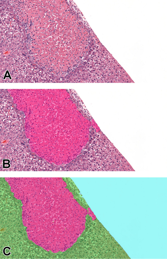
A, Area of necrosis in liver tissue. B, Partial annotations performed only on the lesion, pink: necrosis. C, Full 512 × 512 tiles where blue represents background, green: normal tissue, and pink: necrosis. Images are snapshots taken at ×10 magnification.

The results of lesion detection in the brain tissue are comparable to the results of the rest of the tissues, yet in the brain data set, there were only 70 tiles available for evaluation and the extent of the data is not sufficient to draw significant conclusions. Hence, in the remaining experiments, the heart, lung, liver, and kidney tissues are considered, and brain tissue excluded.

Impact of use of image augmentation strategies

Data augmentation techniques are frequently used to prevent overfitting of neural networks.⁵³ Techniques applied herein include geometric spatial augmentation, elastic deformation, and color augmentation. A meta-analysis of the effects that varying augmentation parameters had on the performance of models was investigated using the consolidated lesion data sets from the various organs. All of the data sets had 3 classes of interest: background, tissue, and lesion, where the background class is ignored as it represents the area on the slide outside the tissue, the tissue class represents normal tissue, and the lesion class represents all the lesions that are annotated in that tissue. This meta-analysis provided insight into the value of each augmentation approach on model performance.

Geometric augmentation

Figure 7 illustrates the average F1 score achieved across all models evaluated with geometric variation enabled (on) and disabled (off). Geometric augmentations are generally characterized by their ease of implementation. It is evident from experimental results that this data preprocessing step can yield positive effects with very little resources required. This form of augmentation presents a good solution when positional biases may be present in the training data.⁵⁴

Figure 7.

Average F1 scores for consolidated lesions across all convolutional neural network models investigated illustrating the impact of geometric augmentation for each of the organs: heart, lung, kidney, and liver.

Elastic deformation

The next augmentation technique investigated was elastic deformation. While geometric augmentation is generally a simple transformation of the image data, elastic deformation is a more fundamental distortion of the input training data, generating distorted variants of the input. These distortions can potentially lead to the presentation of artificial scenarios to the models potentially negatively impacting the training process. The distortions used in this work are subtle. When assessing the average F1 scores across all of the models, elastic deformation showed improved performance on the lung data set (Figure 8) but the rest of the data sets were negatively affected.

Figure 8.

Average F1 score for consolidated lesions across all of the convolutional neural network models investigated for the impact of elastic deformation for each of the organs: heart, lung, kidney, and liver.

Color augmentation

Similar but nonidentical color appearances are generated due to staining process variation between different pathology laboratories. Figure 9 illustrates the color variation observed across the 4 data sets used herein. The heart and lung data sets were collated from a single data source, while kidney and liver tissue data were collected from multiple sources. Due to possible color variance of the digital slides collected between laboratories, models trained with images from one organization might underperform on unseen images from another. Several techniques have been proposed to reduce the generalization error, mainly grouped into 2 categories: color augmentation and color normalization. As Figure 10 shows, the result of color augmentation is positive on the performance for all of the organs, except for the heart. Kidney and liver data sets are collected from multiple sources and therefore have inherent color variation in the data. The validation set is a subset of the same data set; hence, it has a high level of heterogeneity and generalization of the model has a positive impact on the results. The lung and heart data sets are generated from a single source; therefore, the validation set data from which the models are evaluated are not as diverse. Hence, the generalization effect of color augmentation on those data sets might not be visible in the results. Nevertheless, the lung data set demonstrated a positive impact on model performance when color augmentation is applied. Color augmentation applied to the heart data set had a negative impact, and when reviewing the results we identified that some of the lesions classified might be detected via tinctorial changes and color as such are missed when color augmentation is used.

Figure 9.

Average F1 score for consolidated lesions across all of the convolutional neural network models investigated for the impact of color augmentation for each of the organs: heart, lung, kidney, and liver.

Figure 10.

Illustration of the visual variation observed across the different data sets at ×10. As heart (A) and lung (B) originate from a single lab, the variation in color is less than that in kidney (C) and liver (D), which have originated from multiple contributing laboratories. Images are snapshots taken at ×10 magnification.

Optimal model architecture selection

Once optimal parameters for comparative review were selected based on the meta-analysis results, the CNN architecture was chosen. Numerous CNN segmentation model architectures exist, and many have been applied to tasks within the medical domain. Over the course of our research, we have reviewed and selected 10 architectures to include in Patholytix AI (Table 3). These models all operate on the same basic goal, to assign each pixel in an image to one of the annotated categories observed during training. The structure of the image segmentation models can be broken down into 2 parts. The first part, the encoder, learns the features that distinguish between the tissue classes. The second part, the decoder, learns how to take the encoded features and use them to classify each image pixel into one of the classes (resulting in a segmented image). Our model selection is based on popular image segmentation architectures and specifically those that have proven successful on histology samples. The models utilized include FCN8/FCN16,^25,26 U-net,²⁹ and DeepLabV3Plus.²⁸ For the U-Net architecture, we choose to experiment with different backbone structures including ResNet,^33,34,35 Inception,³⁰ InceptionV3,^31,32 Xception,^36,37 and EfficientNet.³⁸ FCN16 and Inception were then further excluded from the analysis based on comparable performance with the FCN8 and InceptionV3 variants of those models. The remaining list of 6 models evaluated were FCN8, InceptionV3, ResNet50, Xception, DeepLabV3Plus, and Seg_Model. The comparative analysis of their performance on consolidated lesion data sets is illustrated in Figure 11. It can be observed that the Seg_Model architecture yields the best performance in all 4 data sets used for the experiments. Xception and InceptionV3 architecture perform equally well on the liver data set but have significantly lower results on the heart, lung, and kidney data sets.

Figure 11.

Illustration of maximum F1 scores achieved for each model, across all configurations attempted, evaluated on consolidated lesions from the heart, kidney, liver, and lung.

Multi-Magnification architecture evaluation

Multi-magnification models make use of the different image magnification layers in a WSI. The use of different levels of magnification allows the model to extract contextual information around the point of interest, which may not be possible to detect at a single magnification. To evaluate the effect of different multi-magnification architectures on the performance of consolidated lesion detection tasks, experiments were performed with 1, 2, and 3 levels of magnification. The base magnification layer of ×10 was used for all the experiments, where 2 layers were used, information from ×5 magnification was also included. Similarly, where 3 layers were used, information from the ×5 and ×2.5 layers were added to the training data. Initially, the experiments were run without image augmentation to assess the performance against the single-magnification approach. All multi-magnification models are constructed using EfficientNetB0 as the encoder similar to the Seg_Model since it was shown to have the best overall performance in the single-magnification level experiments. The results were evaluated for 4 different tissue types and 2 multi-magnification architectures were evaluated.

Table 4 presents the summary of the results. It is evident from this analysis that kidney lesion classification, in particular, was improved for lesion detection when using multi-magnification approaches. Results on the heart data set showed improvement where the F1 score increased from 0.666 on a single-magnification architecture to 0.703 with 2 magnification layers used. In contrast, a significant benefit was not observed in the liver or lung, whereby largely similar results to the single-magnification alternative were observed. The improvements observed in the kidney and heart are only observed with the MESD architecture. Interestingly, the MEMD multi-magnification model architecture either did not improve the results or showed lower results than the single-magnification equivalent. A marked improvement of the F1 score can be observed when using the MESD multi-magnification architecture for the classification of kidney lesions where the result was improved from 0.628 to 0.717. This can potentially be attributed to the complex and distinct morphologies of the main components of the renal parenchyma (tubules–glomeruli–vessels). To investigate if the multi-magnification model can improve the results further, the best augmentation configurations observed in single-magnification experiments were applied to 1 heterogeneous (kidney) and 2 homogeneous (liver, heart) tissue organs, the results of which are summarized in Table 5.

Table 4.

Maximum F1 Scores Achieved on Generalized (Consolidated) Lesion Detection Task for Each Organ Across Single- and Multi-Magnification Models.^a

Organ	Seg_Model (1 layer)	MESD (2 layers)	MESD (3 layers)	MEMD (2 layers)	MEMD (3 layers)
Kidney	0.628	0.678	0.717	0.652	0.228
Lung	0.633	0.621	0.633	0.431	0.021
Liver	0.764	0.756	0.683	0.620	0.568
Heart	0.666	0.703	0.666	0.628	0.379
Brain	0.661	0.608	0.517	0.536	0.315

^a All the results are shown without augmentation and class balancing steps to have an equivalent baseline comparison of the architectures.

Table 5.

F1 Scores Achieved Using MESD Model Architecture on Consolidated Lesions for Selected Organs With 1, 2, and 3 Magnification Layers With the Best Augmentation Configurations Found in Single-Magnification Experiments.

Organ	Augmentation	Seg_Model (1 layer)	MESD (2 layers)	MESD (3 layers)
Kidney	geometric, class balancing	0.778	0.839	0.825
Liver	geometric, class balancing, elastic deformation	0.773	0.742	0.734
Heart	geometric, class balancing	0.778	0.734	0.727
Lung	color, geometric, class balancing, elastic deformation	0.765	0.825	0.803

By using the best augmentation configuration derived from the experiments performed on a single-magnification model, an improvement over all of the organs was observed compared to unaugmented analysis. With augmentation, all the data sets had an F1 score above 0.77, and without augmentation, the F1 scores varied between 0.628 and 0.764. When comparing overall results without any augmentation and utilizing the best-performing augmentation parameters, the optimal augmentation improved results by 9% using 1 magnification layer, by 6% using 2 magnification layers, and by 7% using 3 magnification layers as input data for the classifier. In comparison to the best single-magnification results, MESD shows the most improvement on lesion detection in kidney tissues where the F1 score is increased by 6% and 5%, respectively, when using 2 and 3 magnification layers.

Pixel-level lesion segmentation results of lung tissue using 1, 2, and 3 magnification layers to train the classifier is illustrated in Figure 12. Single-magnification results show overdetection of the lesion class, whereas 2- and 3-layer model architectures are shown to refine the detected lesion area in concordance with the annotation provided by the pathologist. The 3-layer model appears to under-detect some lesion areas; therefore, a lower F1 score is observed when compared with the 2-layer multi-magnification architecture results.

Figure 12.

Illustration of segmentation prediction by the application of single- and multiple magnification layers using best augmentation configuration. From left to right: (A) original lung tissue, annotation overlaid over tissue. B, Seg_Model results with 1 magnification layer, MESD with 2 magnification layers, and MESD with 3 magnification layers. Images are snapshots taken at ×10 magnification. Green: Normal tissue; Red: Lesions (infiltrate).

Figure 13 illustrates the multiclass segmentation prediction results of the kidney tissue using both single and multiple magnifications. It can be observed that lesion areas that are not detected in the single-layer model architecture are detected when more context is added from the higher magnification layer.

Figure 13.

Illustration of segmentation prediction by the application of single- and multiple magnification layers using best augmentation configuration. From left to right: (A) original kidney tissue, annotation overlaid over tissue. B, Seg_Model results with 1 magnification layer, MESD with 2 magnification layers, and MESD with 3 magnification layers. Images are snapshots taken at ×10 magnification. Red: Lesions (lymphocytes); Blue: Background.

When a third layer of magnification is included in the training data, the areas that are detected as lesions are amplified when compared to the 2-layer approach; therefore, in this scenario, adding more context from the third layer (×2.5 in this analysis) leads the model to over-detect the lesion. This can be observed in Table 6, where both precision and sensitivity have improved when using multiple magnification layers for the kidney; however, the 3 magnification layers result in lower precision, but higher sensitivity when compared to the model using 2 magnification layers.

Table 6.

Precision, Sensitivity, and F1 Scores Achieved for Single- and Multi-Magnification Models for Kidney.

Magnification layers	Precision	Sensitivity	F1
1	0.733	0.829	0.778
2	0.830	0.848	0.839
3	0.801	0.852	0.825

Note: Bold indicates highest scores achieved per parameter

Section 2: Data Set Optimization Strategy and Classification Performance

Performance on individual lesion detection and identification using a single CNN model

The capability of a single classifier to identify all the annotated lesions in a single tissue type was investigated. As illustrated by the results for the heart data set (Figure 14 ), poor performance was generally observed when using this approach. In many cases, lesions were detected as “normal tissue,” resulting in a high level of FNs. It is anticipated that performance was affected by the extent of the representation of individual lesion classes in the data set (fibrosis; hemorrhage; infiltrate, mononuclear (foamy); bacterial colonies) where there were less than 10 examples of each class available in the training data set. Confusion was also noted between classes (mineralization, cardiomyocyte; mineralization, media, artery) where pixels of one class are classified as the other.

Figure 14.

Confusion matrix of variant classes in the heart lesion annotation using Seg_Model classification. Left to right: For each lesion class, the proportions of the pixels classified as each of the available classes are shown (max = 1).

Performance on consolidated lesion detection using CNN models

To mitigate the problems identified in the multiclass classifier, consolidated training data sets, where all lesions were consolidated into a single “lesion” class, were created. These consolidated data sets consist of 3 classes: background, tissue, and lesion. The lesion class is a combination of all lesion classes in a given organ data set. Comparison between the classifier created for the heart using individual lesion classes and a single combined lesion classifier can be seen in Figure 15.

Figure 15.

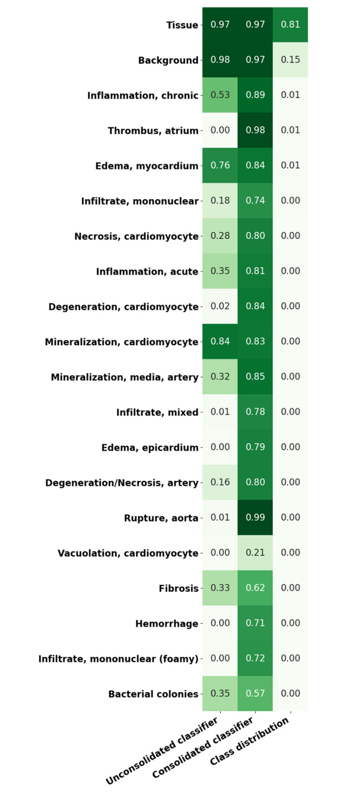
Representation of sensitivity in unconsolidated/consolidated classes of heart tissue using Seg_Model (max = 1). The first column shows the lesion detection rate in an unconsolidated annotation set where each class is to be detected individually. The second column shows the equivalent results from the consolidated lesion classifier set where all of the lesion classes are combined into a single class. The last column illustrates the proportion of the data set that each of the classes represent. All of the results are shown on the complete annotated data set, including training, testing, and validation data.

When lesions are consolidated into a single lesion class, a significant improvement in the detection of lesions in general is observed, the overall lesion detection rate in heart increased from 23% to 76.4% following consolidation. Figures 16 and 17 illustrate the mask predictions generated for lesions within the kidney and liver and the heart and lung slides that were achieved using the consolidated lesion training set. In particular, we note a measured improvement in the detection of poorly represented lesions by these models, with the detection of each of the classes individually improved by an average of 53%.

Figure 16.

Tissue/associated prediction masks for the kidney and liver achieved with the best-performing classifier on the consolidated lesion training set. Hematoxylin and eosin, ×10 magnification. (A) Casts, medullary tubules/kidney; (B) Hypertrophy, centrilobular/liver; (C) Prediction mask for lesions (red), normal tissue (green); and (D) Prediction mask for lesions (red), normal tissue (green).

Figure 17.

Tissue/associated prediction masks for the lung and heart achieved with the best-performing classifier on the consolidated lesion training set. (A) Congestion and edema/lung; (B) Inflammation, chronic/heart; (C) Prediction masks for lesions (red), normal lung tissue (green); and (D) Prediction masks for lesions (red), normal heart tissue (green). Images are snapshots taken at ×10 magnification.

This consolidation approach was applied across all data sets, as it was hypothesized that it may be beneficial where tinctorial changes such as basophilia in the kidney tubules, hepatocellular cytoplasmic alteration, or minimal hepatocellular hypertrophy may be challenging to detect, especially when they are observed early in their development timeline.

To investigate the potential impact of this approach, single lesion analysis was performed on selected findings from each of the organs and compared to the average consolidated result for lesion detection.

Performance on single lesion detection and identification using CNN models

We observed a varying level of performance in results when identifying individual lesions (Figure 18), with some lesion classifications performing almost perfectly (the F1 score for fatty change and necrosis in liver tissue was >0.97) where other lesions were poorly determined in comparison to the consolidated lesion detection model (necrosis in the heart tissue and mononuclear infiltrate in the lung tissue showed resultant F1 scores of <0.5).

Figure 18.

F1 score for consolidated lesion detection for each of the organs, heart, lung, kidney, and liver, and individual class analysis via a “one-versus-all” classification approach using Seg_Model/MESD, where optimal.

Overall, liver and kidney nonclinical tissue analysis outperformed the heart, lung, and brain in terms of the classification capabilities of the CNN, which can largely be attributed to the extensive volume of annotated lesions within those data sets. When comparing the proportion of annotated pixels to the classification performance (Figure 19), it can be observed that high F1 scores were achieved when the extent of lesions in the training set exceeds 10 million pixels, this threshold is dependent on lesion representation in comparison to the normal classes.

Figure 19.

Relationship between the extent of representation of a specific lesion in the training set (number of pixels) and the classification performance of the model for that lesion in the validation data set (best F1 score) is graphically represented. A 95% confidence interval was applied (dotted line).

Discussion

The application of AI in toxicology pathology and safety assessment is gaining significant momentum due to the advancements and techniques in the field of digital pathology. With the aim of developing optimized algorithms for automated lesion detection in nonclinical organs, and to streamline workflow for pathologists, a multidisciplinary effort involving teams from 3 different organizations including pathologists, data scientists, and AI engineers was undertaken as described herein. The success of any machine learning project is generally impacted by the quality and quantity of available data. The TG-GATEs data set is a highly comprehensive collection of nonclinical toxicologic studies that offers an extensive range of lesions and severity across both liver and kidney data sets, while also providing diversity in the appearance of staining and processing. In comparison to the highly curated and consistent internal R&D data set analyzed, the TG-GATEs data set has accompanying metadata that do not accurately correlate, either in range of lesions present or extent of lesion severity, with findings visually apparent within each slide. This discrepancy was corrected in our internal data sets once peer-reviewed by pathologists as part of this work. Standardization of ontologies is critical when considering the use of data from multiple origins and we have adhered to SEND and INHAND standards⁴¹ to ensure standardization and interoperability of our consolidated data sets. To achieve the broadest coverage of potential lesions assessed, along with degrees of severity, contributing pathologists were tasked with reviewing each of the studies, peer reviewing, and updating all findings, along with annotating examples of lesions in those tissues. For this study, pathologists have spent approximately 650 hours on this endeavor. Over 3600 slides have been reviewed, of which 1300 were annotated, generating 17,000 annotated tiles, with over 2 billion annotated pixels containing approximately 200 million annotated lesion pixels. Three different variants of the data sets were generated to explore the impact of different consolidation approaches on the classifiers ability to detect and identify lesions. The first approach was to train a single model on all of the lesions available for a particular tissue type. Subsequently, the variants of each data set were generated to combine all of the lesions into a single class and to pick out the lesion classes of interest and train a classifier to identify only those. The classifiers are evaluated based on the blinded set of tiles that consisted of 15% of the total tiles available with annotations. Despite the large amounts of annotated tiles, annotation bias may be observed in generated classifiers depending on the validation technique used to assess classifier performance due to the fact that validation data are annotated by the same pathologist as the training data. Subsequent work from this research aims at developing validation studies from diverse sources, which are annotated but not used for training.

Augmentation techniques including geometric augmentation and elastic deformation were shown to have a varied effect on the F1 scores of organ-specific classifiers. Geometric augmentation improved the F1 scores compared to when no augmentation was used; however, elastic deformation only improved F1 scores on the lung data set. This was expected, as a minimal representation of lesions and annotations were present in the lung cohort, which in turn highlighted the benefits of elastic deformation and generation of simulated realistic deformation examples provided when limited training data are available. For color augmentation, it was evident that the heart slides were carefully curated from a single lab source and digitized using a single scanner, where limited variation in staining intensity or color variation is observed. Whereas for both the liver and kidney data sets, a variety of sources were used in the compilation of the cohorts where disparity is apparent. This lack of standardization within slide preprocessing, owing to variations in staining protocols and digitization, likely leads to color imbalances and varying tinctorial differences across the cohort. This is visually illustrated in Figures 9 and 10, which subsequently showed the increased benefit in F1 scores from color augmentation. Six models were evaluated: FCN8, InceptionV3, ResNet50, Xception, DeepLabV3Plus, and Seg_Model, with Seg_Model providing the most superior results across all organs. This model is an implementation of the Segmentation Models library by Yakubovskiy.⁴² Instead of one single model architecture, this model allows the user, through the use of the hyperparameters, to create an encoder–decoder model based on one of 4 popular architectures: Unet, FPN, Linknet, and PSPNet. These models are then enhanced with a pretrained backbone, which defines the structure of the encoder and, shown by these results, allows it to benefit from the features already learned from these models that have been pretrained on very large data sets.

Using Seg_Model, the application of multi-magnification training was assessed. In contrast to the findings reported in Ho et al,²⁴ where MEMD performed better than MESD, we have found that additional contextual information is more useful when concatenated at the encoder level rather than at the decoder level. Another potential reason why MESD excelled in this situation may be due to the smaller number of available training examples, in comparison to data sets previously reported by Ho and colleagues.²⁴ By excluding decoders at lower magnification levels, MESD required less training examples.

Based on the experiments performed without augmentation (Table 5), improvements are evident on the kidney and heart data when using the MESD model; however, once the standardized augmentation techniques were applied, only the kidney and lung had observable beneficial effects from the incorporation of MESD (Table 5). Detecting lesion boundaries in the lung tissue was improved when 2 magnification layers were included to train the algorithm, as can be observed from the examples in Figure 11. Kidney classification using 2 magnification layers also had an ameliorative effect on the F1 score as opposed to a single layer, or even 3 layers; this classification can be visually observed in Figure 12. This result suggests that the advantage offered by adding additional contextual information during the training of AI models is largely dependent on the tissue architecture and heterogeneity of the structures. Any improvement of model classification performance observed while using multi-magnification approaches is deemed to vary significantly depending on the organ type. However, in these certain scenarios, the application of multi-magnification approaches can prove very beneficial.

The development of a multiclass classifier that facilitates the detection of multiple lesion types concurrently is attractive due to its computational efficiency. When a model was trained on a data set where lesions are combined into a single class, a 53% improvement was seen in the detection of lower represented lesions. This gives rise to the theory that the consolidated classifier may have the ability to generalize beyond training examples. In the training data, representation of certain lesion classes was very low, yet in the validation data, the model detects those lesions reasonably well (Figure 14). This means that the consolidated lesion models, based on the data available to us, have the potential to generalize for unseen examples; however, as an external annotated data set is not available to fully evaluate the generalization capability of the classifiers, further evaluation will be required to determine the potential of the models to generalize on data sets from unseen sources.

There is a general trend observable within the data where the greater the level of representation of a given lesion in the annotation set, the higher the likelihood of detection in validation data (Figure 18). Outliers have been observed with certain lesions substantially over and under achieving with respect to the general trend, even when class balancing is applied. This is due to the limited array of examples that can be generated using class balancing, which cannot generate true diversity. Mineralization in the kidney, which delivered high-yielding classification performance from a relatively low number of annotated pixels, routinely presents as basophilic deposits that may involve the tubule epithelia and/or the interstitium, is often an evident and apparently easy finding to visually interpret. However, more challenging changes such as tubular degeneration or tubular basophilia, which may already be very subtle to distinguish from a pathologist’s perspective, when the severity grade is minimal, still show a poorer performance despite having a higher number of pixels annotated than mineralization. Similarly, centrilobular hepatocellular hypertrophy, with large numbers of annotations, can be quite a subtle change when the degree of severity is low, thus subject to interobserver variability and hence not as easily predicted by the models. In the lung, confusion between real infiltrates of mononuclear cells or eosinophils and bronchus-associated lymphoid tissue seemingly lowered the performance score. Interestingly, the F1 score for heart, “infiltrate, mononuclear” is low, but after extraction and review of the annotated tiles, it was evident that there was confusion with blood vessels, and confusion between the “inflammation, chronic class” and the “infiltrate, mononuclear” class, a result which is not so surprising, given that mononuclear cells are very often a feature of chronic inflammation. Overall, the relationship between the F1 score and the number of pixels annotated appears proportional and is affected not only by the extent of the annotation set and representation of the lesions (number of pixels) but also by confusion between similar classes/between normal components of the tissue that may appear lesion-like to the model. This is further compounded by the subtlety of the change observed in the tissue (subtle morphological variation, faint tinctorial changes). This emphasizes the shortcomings observed within the data set for lung, which had a lower number of minimally represented lesions, which may be attributed to the lower F1 scores observed. Future improvements for this research will focus on the enhancement of these models without the need for further annotations. The robustness of models produced from DL strategies will vary depending on the quality and extent of curated content used for training. Robust training data sets will be required from a diversity of contributing laboratories to ensure the general applicability of models outside the data they are generated from. We believe that large repositories of consolidated data cohorts are required. Initiatives like the Big Data for Better Outcomes initiative⁵⁵ will make these goals more attainable for model developers universally and will do a lot to enhance and scale validation efforts in this regard. Even if the data deficit can be addressed, we believe that new models need to be proposed that can robustly detect “unseen” lesion examples based on a generalized model of normal tissues; we also believe that approaches such as multiple instance learning⁵⁶ can be leveraged to utilize sparsely annotated data sets and hence reduce the overheads on pathologist time required to annotate copious examples of various lesions.

Conclusion

Overall, herein, we have demonstrated that generalized lesion classifiers trained on examples of multiple different lesions can work effectively in determining lesions in validation cohorts. Additionally, models of this nature can potentially generalize well, efficiently detecting poorly represented lesions in the training data. Similarly, we have demonstrated that models can be developed to detect specific lesions in specific organs; however, their performance is contingent on the extent of representation of that lesion in the training data and potentially on the subtlety of the lesion in question.

We have provided a framework on how researchers in this space can develop and optimize CNN models for specific nonclinical tissues, incorporating a variety of enhancement strategies including class balancing, geometric, and color augmentation techniques. Finally, we have illustrated the potential of multi-magnification models in certain limited evaluations and have observed its benefit in lesion determination in the kidney, where normal morphology is complex and structural context from lower resolutions may enhance detection.

References

- 1. Center for Food Safety and Applied Nutrition O of FAS. Redbook 2000: IV.C.4.a. Subchronic Toxicity Studies with Rodents. U.S. Food & Drug Administration; 2003. https://www.fda.gov/regulatory-information/search-fda-guidance-documents/redbook-2000-ivc4a-subchronic-toxicity-studies-rodents#test
- 2. Clarke M, Graham TM. How do we train and retain the new generation of pathologists? Br J Healthcare Manage. 2020;26(4):1–3. doi:10.12968/bjhc.2020.0017 [Google Scholar]
- 3. Haenssle HA, Fink C, Schneiderbauer R, et al. Man against machine: diagnostic performance of a deep learning convolutional neural network for dermoscopic melanoma recognition in comparison to 58 dermatologists. Ann Oncol. 2018;29(8):1836–1842. doi:10.1093/annonc/mdy166 [DOI] [PubMed] [Google Scholar]
- 4. Azam AS, Miligy IM, Kimani PK, et al. Diagnostic concordance and discordance in digital pathology: a systematic review and meta-analysis. J Clin Pathol. 2020. doi:jclinpath-2020-206764 [DOI] [PMC free article] [PubMed] [Google Scholar]
- 5. Turner OC, Aeffner F, Bangari DS, et al. Society of Toxicologic Pathology Digital Pathology and Image Analysis Special Interest Group Article*: opinion on the application of artificial intelligence and machine learning to digital toxicologic pathology. Toxicol Pathol. 2020;48(2):277–294. doi:10.1177/0192623319881401 [DOI] [PubMed] [Google Scholar]
- 6. Nirschl JJ, Janowczyk A, Peyster EG, et al. A deep-learning classifier identifies patients with clinical heart failure using whole-slide images of H and E tissue. PLoS One. 2018;13(4):e0192726. doi:10.1371/journal.pone.0192726 [DOI] [PMC free article] [PubMed] [Google Scholar]
- 7. Steiner DF, MacDonald R, Liu Y, et al. Impact of deep learning assistance on the histopathologic review of lymph nodes for metastatic breast cancer. Am J Surg Pathol. 2018;42(12):1636–1646. [DOI] [PMC free article] [PubMed] [Google Scholar]
- 8. Campanella G, Hanna MG, Geneslaw L, et al. Clinical-grade computational pathology using weakly supervised deep learning on whole slide images. Nat Med. 2019;25(8):1301–1309. [DOI] [PMC free article] [PubMed] [Google Scholar]
- 9. Saima R, Iftikhar MA, Mourelatos Z. Prediction of overall survival and molecular markers in gliomas via analysis of digital pathology images using deep learning. arXiv preprint arXiv:1909.09124. 2019.
- 10. Achi HE, Belousova T, Chen L, et al. Automated diagnosis of lymphoma with digital pathology images using deep learning. Ann Clin Lab Sci. 2019;49(2):153–160. [PubMed] [Google Scholar]
- 11. Jarrahi MH. Artificial intelligence and the future of work: human-AI symbiosis in organizational decision making. Business Horizons. 2018;61(4):577–586. doi:10.1016/j.bushor.2018.03.007 [Google Scholar]
- 12. Sarwar S, Dent A, Faust K, et al. Physician perspectives on integration of artificial intelligence into diagnostic pathology. NPJ Digit Med. 2019;2(1):28. doi:10.1038/s41746-019-0106-0 [DOI] [PMC free article] [PubMed] [Google Scholar]
- 13. Kalra S, Tizhoosh HR, Shah S, et al. Pan-cancer diagnostic consensus through searching archival histopathology images using artificial intelligence. NPJ Digit Med. 2020;3(1). doi:10.1038/s41746-020-0238-2 [DOI] [PMC free article] [PubMed] [Google Scholar]
- 14. Hägele M, Seegerer P, Lapuschkin S, et al. Resolving challenges in deep learning-based analyses of histopathological images using explanation methods. Scientific Rep. 2020;10(1):6423. doi:10.1038/s41598-020-62724-2 [DOI] [PMC free article] [PubMed] [Google Scholar]
- 15. Heinemann F, Birk G, Stierstorfer B. Deep learning enables pathologist-like scoring of NASH models. Scientific Rep. 2019;9(1):1845. doi:10.1038/s41598-019-54904-6 [DOI] [PMC free article] [PubMed] [Google Scholar]
- 16. Halicek M, Shahedi M, Little JV, et al. Head and neck cancer detection in digitized whole-slide histology using convolutional neural networks. Scientific Rep. 2019;9(1). doi:10.1038/s41598-019-50313-x [DOI] [PMC free article] [PubMed] [Google Scholar]
- 17. Serag A, Ion-Margineanu A, Qureshi H, et al. Translational AI and deep learning in diagnostic pathology. Front Med. 2019;6:185. doi:10.3389/fmed.2019.00185 [DOI] [PMC free article] [PubMed] [Google Scholar]
- 18. Bertram CA, Aubreville M, Gurtner C, et al. Computerized calculation of mitotic count distribution in canine cutaneous mast cell tumor sections: mitotic count is area dependent. Vet Pathol. 2020;57(2):214–226. doi:10.1177/0300985819890686 [DOI] [PubMed] [Google Scholar]
- 19. Sonigo C, Jankowski S, Yoo O, et al. High-throughput ovarian follicle counting by an innovative deep learning approach. Scientific Rep. 2018;8(1):13499. doi:10.1038/s41598-018-31883-8 [DOI] [PMC free article] [PubMed] [Google Scholar]
- 20. Rudmann DG, Marxfield H, et al. European Society of Toxicologic Pathology. 2019. [Google Scholar]
- 21. Xue Y, Ray N. Cell detection in microscopy images with deep convolutional neural network and compressed sensing. Published Online August 10, 2017. http://arxiv.org/abs/1708.03307
- 22. Das K, Karri SPK, Guha Roy A, Chatterjee J, Sheet D. Classifying histopathology whole-slides using fusion of decisions from deep convolutional network on a collection of random multi-views at multi-magnification. In: Proceedings – International Symposium on Biomedical Imaging. IEEE Computer Society. 2017:1024–1027. doi:10.1109/ISBI.2017.7950690. [Google Scholar]
- 23. Wang Y, Choi EJ, Choi Y, et al. Breast cancer classification in automated breast ultrasound using multiview convolutional neural network with transfer learning. Ultrasound Med Biol. 2020;46(5):1119–1132. doi:10.1016/j.ultrasmedbio.2020.01.001 [DOI] [PubMed] [Google Scholar]
- 24. Ho DJ, Yarlagadda DVK, D’Alfonso TM, et al. Deep multi-magnification networks for multi-class breast cancer image segmentation. Published Online October 28, 2019. http://arxiv.org/abs/1910.13042 [DOI] [PMC free article] [PubMed]
- 25. Shelhamer E, Long J, Darrell T. Fully convolutional networks for semantic segmentation. IEEE Trans Pattern Anal Mach Intell. 2017;39(4):640–651. doi:10.1109/TPAMI.2016.2572683 [DOI] [PubMed] [Google Scholar]
- 26. Bug D, Feuerhake F, Oswald E, Schüler J, Merhof D. Semi-automated analysis of digital whole slides from humanized lung-cancer xenograft models for checkpoint inhibitor response prediction. Vol 10; 2019. www.oncotarget.com [DOI] [PMC free article] [PubMed] [Google Scholar]
- 27. Badrinarayanan V, Kendall A, Cipolla R. SegNet: a deep convolutional encoder-decoder architecture for image segmentation. IEEE Trans Pattern Anal Mach Intell. 2017;39(12):2481–2495. doi:10.1109/TPAMI.2016.2644615 [DOI] [PubMed] [Google Scholar]
- 28. Chen L-C, Zhu Y, Papandreou G, Schroff F, Adam H. Encoder-decoder with atrous separable convolution for semantic image segmentation. Published Online February 7, 2018. http://arxiv.org/abs/1802.02611
- 29. Ronneberger O, Fischer P, Brox T. U-Net: convolutional networks for biomedical image segmentation. Published Online May 18, 2015. http://arxiv.org/abs/1505.04597
- 30. Szegedy C, Liu W, Jia Y, et al. Going deeper with convolutions. In: Proceedings of the IEEE Conference on Computer Vision and Pattern Recognition, San Juan, Puerto Rico, USA, June, 17-19, 2015:1–9. [Google Scholar]
- 31. Szegedy C, Vanhoucke V, Ioffe S, Shlens J, Wojna Z. Rethinking the Inception architecture for computer vision. In: Proceedings of the IEEE Computer Society Conference on Computer Vision and Pattern Recognition. IEEE Computer Society; 2016:2818–2826. doi:10.1109/CVPR.2016.308 [Google Scholar]
- 32. Abidin AZ, Deng B, DSouza AM, et al. Deep transfer learning for characterizing chondrocyte patterns in phase contrast X-ray computed tomography images of the human patellar cartilage. Computer Biol Med. 2018;95:24–33. doi:10.1016/j.compbiomed.2018.01.008 [DOI] [PMC free article] [PubMed] [Google Scholar]
- 33. Habibzadeh Motlagh M, Jannesari M, Rezaei Z, Totonchi M, Baharvand H. Automatic white blood cell classification using pre-trained deep learning models: ResNet and Inception. In: Tenth International Conference on Machine Vision (ICMV 2017). 2017, Vienna, Austria; 2018:105. doi:10.1117/12.2311282 [Google Scholar]
- 34. He K, Zhang X, Ren S, Sun J. Deep residual learning for image recognition. In: Proceedings of the IEEE Computer Society Conference on Computer Vision and Pattern Recognition. IEEE Computer Society. 2016:770–778. doi:10.1109/CVPR.2016.90 [Google Scholar]
- 35. Xie B, He X, Huang W, et al. Clinical image identification of basal cell carcinoma and pigmented nevi based on convolutional neural network. J Centr South Univers (Med Sci). 2019;44(9):1063–1070. doi:10.11817/j.issn.1672-7347.2019.190205 [DOI] [PubMed] [Google Scholar]
- 36. Yang A, Yang X, Wu W, Liu H, Zhuansun Y. Research on feature extraction of tumor image based on convolutional neural network. IEEE Access. 2019;7:24204–24213. doi:10.1109/ACCESS.2019.2897131 [Google Scholar]
- 37. Chollet F. Xception: deep learning with depthwise separable convolutions. In: Proceedings of the IEEE Conference on Computer Vision and Pattern Recognition, San Juan, Puerto Rico, USA, June 17-19, 2017:1251–1258. [Google Scholar]
- 38. Tan M, Le QV. EfficientNet: rethinking model scaling for convolutional neural networks. Published Online May 28, 2019. http://arxiv.org/abs/1905.11946
- 39. Open TG-Gates Database. Accessed July 30, 2020. http://toxico.nibiohn.go.jp/english/
- 40. Igarashi Y, Nakatsu N, Yamashita T, et al. Open TG-GATEs: a large-scale toxicogenomics database. Nucleic Acids Res. 2015;43(D1):D921–D927. doi:10.1093/nar/gku955 [DOI] [PMC free article] [PubMed] [Google Scholar]
- 41. Mann PC, Vahle J, Keenan CM, et al. International harmonization of toxicologic pathology nomenclature: an overview and review of basic principles. Toxicol Pathol. 2012;40(suppl 4):7S–13S. doi:10.1177/0192623312438738 [DOI] [PubMed] [Google Scholar]
- 42. Yakubovskiy P. Segmentation models, GitHub repository. Published 2019. Accessed July 30, 2020. https://github.com/qubvel/segmentation_models
- 43. Russakovsky O, Deng J, Su H, et al. Imagenet large scale visual recognition challenge. Int J Com Vis. 2015;115(3):211–252. [Google Scholar]
- 44. He K, Zhang X, Ren S, Sun J. Delving deep into rectifiers: surpassing human-level performance on Imagenet classification. In: Proceedings of the IEEE International Conference on Computer Vision (ICCV) [Internet]. February 6, 2015; http://arxiv.org/abs/1502.01852 [Google Scholar]
- 45. Lin T-Y, Goyal P, Girshick R, He K, Dollár P. Focal loss for dense object detection. arXiv preprint [Internet]. August 7, 2017; http://arxiv.org/abs/1708.02002 [DOI] [PubMed]
- 46. Zarella MD, Breen DE, Plagov A, Garcia FU. An optimizedcolor transformation for the analysis of digital images of hematoxylin & eosin stained slides. J Pathol Inform. 2015;6:33. [DOI] [PMC free article] [PubMed] [Google Scholar]
- 47. Wang L, Weinan Li, Yan K. Data fusion network for instance segmentation. In: International Conference on Health Information Science. Springer; 2018:175–182. [Google Scholar]
- 48. Chang HH, Zhuang AH, Valentino DJ, Chu WC. Performance measure characterization for evaluating neuroimage segmentation algorithms. NeuroImage. 2009;47(1):122–135. doi:10.1016/j.neuroimage.2009.03.068 [DOI] [PubMed] [Google Scholar]
- 49. Udupa JK, LeBlanc VR, Zhuge Y, et al. A framework for evaluating image segmentation algorithms. Comput Med Imaging Graph. 2006;30(2):75–87. doi:10.1016/j.compmedimag.2005.12.001 [DOI] [PubMed] [Google Scholar]
- 50. Garcia-Garcia A, Orts-Escolano S, Oprea S, Villena-Martinez V, Garcia-Rodriguez J. A review on deep learning techniques applied to semantic segmentation. Published Online April 22, 2017. http://arxiv.org/abs/1704.06857
- 51. Fenster A, Chiu B. Evaluation of segmentation algorithms for medical imaging. In: Annual International Conference of the IEEE Engineering in Medicine and Biology – Proceedings. Vol 7. Institute of Electrical and Electronics Engineers Inc.; 2005:7186–7189. doi:10.1109/iembs.2005.1616166 [DOI] [PubMed] [Google Scholar]
- 52. Buda M, Maki A, Mazurowski MA. A systematic study of the class imbalance problem in convolutional neural networks. Neural Netw. 2018;106:249–259. doi:10.1016/j.neunet.2018.07.011 [DOI] [PubMed] [Google Scholar]
- 53. Wong SC, Gatt A, Stamatescu V, McDonnell MD. Understanding data augmentation for classification: when to warp? Published Online September 28, 2016. http://arxiv.org/abs/1609.08764
- 54. Shorten C, Khoshgoftaar TM. A survey on image data augmentation for deep learning. J Big Data. 2019; 6(1). doi:10.1186/s40537-019-0197-0 [DOI] [PMC free article] [PubMed] [Google Scholar]
- 55. About BD4BO, Big Data for Better Outcomes website. Accessed October 13, 2020. https://bd4bo.eu/index.php/about-the-programme/about-bd4bo/
- 56. Lu MY, Williamson DFK, Chen TY, et al. Data efficient and weakly supervised computational pathology on whole slide images. Published Online April 20, 2020. http://arxiv.org/abs/2004.09666 [DOI] [PMC free article] [PubMed]