Wavelet Screening identifies regions highly enriched for differentially methylated loci for orofacial clefts

Abstract

DNA methylation is the most widely studied epigenetic mark in humans and plays an essential role in normal biological processes as well as in disease development. More focus has recently been placed on understanding functional aspects of methylation, prompting the development of methods to investigate the relationship between heterogeneity in methylation patterns and disease risk. However, most of these methods are limited in that they use simplified models that may rely on arbitrarily chosen parameters, they can only detect differentially methylated regions (DMRs) one at a time, or they are computationally intensive. To address these shortcomings, we present a wavelet-based method called ‘Wavelet Screening’ (WS) that can perform an epigenome-wide association study (EWAS) of thousands of individuals on a single CPU in only a matter of hours. By detecting multiple DMRs located near each other, WS identifies more complex patterns that can differentiate between different methylation profiles. We performed an extensive set of simulations to demonstrate the robustness and high power of WS, before applying it to a previously published EWAS dataset of orofacial clefts (OFCs). WS identified 82 associated regions containing several known genes and loci for OFCs, while other findings are novel and warrant replication in other OFCs cohorts.

INTRODUCTION

In mammals, DNA methylation (DNAm) is an epigenetic mark which is essential for normal development and regulates processes such as gene expression, genomic imprinting, X inactivation and the maintenance of genomic integrity. The majority of DNAm is in the form of 5-methylcytosine in a CpG dinucleotide. In the past decade, there has been considerable interest in identifying associations between DNA methylation variation and human disease. Typically, epigenome-wide association studies (EWAS) measure levels of DNAm at CpG sites and compare these between case and control groups. The rationale for conducting an EWAS is that this may identify loci associated with a disease, and thus provide insights into the biological mechanisms involved.

Over the past 30 years, numerous methods have been developed to measure DNAm, varying in resolution from single CpGs to whole-genome coverage (1). In the last decade by far the most common is the Illumina BeadChip array, initially as the 450K (∼450 000 sites) and now the EPIC array (∼850 000 sites). The EPIC array has good genome-wide coverage, covering all RefSeq genes, as well as regions regulating gene expression (ENCODE open chromatin and enhancers, DNase hypersensitive sites and miRNA promoter regions).

Despite these advances, the EPIC 850K still covers only about of the total estimated number of CpGs in the human genome (∼28 million) (2). Furthermore, the use of even sparser methylation platforms, such as 450K, makes it challenging to integrate associations between distant CpGs. Hence, there is a growing need to develop methods that are both robust and versatile in handling DNAm data generated on these sparse platforms that are widely used in many consortia-led epigenome-wide meta-analyses.

Compared to earlier investigations in which CpGs were typically interrogated one at a time, the focus of newer studies is moving toward investigating multiple CpGs simultaneously through testing larger regions of the genome (3–5). This has spurred the development of various approaches to modeling multiple CpGs at a time (4,6,7). One such approach, proposed by Jenkinson and colleagues (8), involves performing regional modeling of blocks of 1 kb of DNA. They showed that blocks of DNAm with high entropy are efficient predictors of important genetic features, for example, topologically associating domains (TADs) (9,10). Even before the work of Jenkinson et al. (8), several authors had already suggested applying regional tests to detect systematic differences in DNAm profile (3,11) or P-value enrichment (12).

Despite these advances in modeling multiple CpGs simultaneously, a limitation of these methods is that they use a fixed region size of 1 kb and do not take the CpG density of the region and the spacing between the CpGs into account (4,13,14). Such approaches to modeling might overlook more complex effects of CpGs, both within and outside of a given CGI, as highlighted by Irizarry et al. (6). A new hybrid approach to modeling DNAm profile called ‘methylated CpGs Set Enrichment Analysis’ (mCSEA) (5) combines the direct estimation of DMRs with a reweighting procedure from a powerful analytical method called Gene-Set Enrichment Analysis (GSEA). Despite a significant improvement in power, there is still the possibility of bias due to the reliance of mGSEA on external information (see Geeleher et al. (15) for additional details).

To address some of these methodological shortcomings, Lee and Morris (16) introduced a method for modeling DNAm profile based on the use of wavelets (17) in a functional mixed-modeling approach. This was a follow-up to the initial work by Morris and Carroll (18). Wavelets are useful mathematical functions for conducting a Fourier-like transform, which, in the current context, can be used to treat an individual’s DNAm profile as a ‘signal’. Importantly, compared to Fourier transform, which requires the signal to be periodic, wavelets (and wavelet transform) can represent a wider variety of signals and can easily be adapted to represent an individual’s DNAm profile. In their paper, Lee and Morris (16) showed that association testing using wavelet transform enables the detection of smaller variations within the DNAm profile compared to previous methods (3,11,12).

Wavelets have been used to analyze different types of omics data, for example, to identify genetic variants associated with chromatin accessibility (19), to investigate DMRs in DNAm data (16) and to screen for risk-conferring variants in genome-wide association studies (GWASes) (20,21). However, the methods described by Jaffe et al. (22) and Lee and Morris (16) are based on a preassigned significance threshold for detecting a difference in DNAm profile across groups of individuals. As this threshold is set a priori by the analyst, it is difficult to compare findings across studies in which different predetermined thresholds have been used. Moreover, such methods fail to take advantage of the joint effects of DMRs that individually do not pass a set significance threshold. Finally, the methods mentioned thus far are computationally intensive and have only been applied to limited datasets (e.g. 141 individuals in Lee and Morris (16)).

To address these shortcomings, we introduce a new wavelet-based approach called Wavelet Screening (WS) for the efficient analysis of data generated on different methylation platforms, irrespective of their probe density. To achieve this, we drew inspiration from the work of Lee and Morris (16) and adapted the analysis criterion of Jenkinson et al. (8) using the Jensen-Shannon distance. To illustrate the utility of WS, we analyzed a previously published EWAS comprising 412 orofacial clefts (OFCs) cases and 456 controls (14). OFCs are relatively common congenital malformations that often require extensive follow-up and treatment from childhood through adolescence (23,24). They are characterized by a strong genetic predisposition based on estimates of heritability and familial recurrence (25–29). It is thus intriguing that the genetic variants identified thus far have only been able to explain a small fraction of the total heritability of OFCs (30).

The phenomenon of missing heritability is not unique to OFCs but has plagued the vast majority of studies aimed at unraveling the genetic underpinnings of complex traits. As environmental factors can induce epigenetic changes, with reported associations between specific genotypes and DNAm levels at CpG sites (i.e. methylation quantitative trait loci (mQTLs); (31,32)), it is conceivable that part of the unexplained causality of OFCs could be accounted for by epigenetic mechanisms (13,33,34). This calls for the development of more flexible and powerful analytic tools to handle different types of omics data (35) in order to capture a greater proportion of the genetic variants potentially missed by conventional methods.

In the present study, DNAm data from babies born with OFCs (cases) and those born without such malformations (controls) were available from a population-based study of OFCs in Norway (14,36). We divided the genomes of the cases and controls into smaller regions and modeled the DNAm profile of each individual using wavelets. Our method enables studying complex effects of DNAm, including the combined effect of several DMRs, instead of only screening for simple systematic differences in DNAm profiles (19). We provide a brief description of the wavelet transform in the Materials and Methods section before outlining the statistical framework for WS and its adaptation to DNAm data.

The remainder of this paper is structured as follows. We first provide a detailed account of each step involved in the modeling scheme of WS in the ‘Materials and Methods’ section, followed by the section ‘Application of Wavelet Screening’ where we present two applications of WS: the first to an existing case-control DNAm dataset of OFCs and the second to a simulated DNAm dataset that mimics a previous study of colon cancer by Irizarry and colleagues (6). In the ‘Results’ section, we present the output of our analyses and the visualization of the results. Finally, in the ‘Discussion’ section, we contrast our findings with another EWAS that used the same OFCs dataset as here (14) and additional studies that have examined other OFCs DNAm datasets.

Application note: WS is distributed as an R package on GitHub (https://github.com/william-denault/WaveletScreening). A comprehensive example of a typical WS run is provided in the description of the main function in the R package.

MATERIALS AND METHODS

Even though WS was originally designed for GWAS, it can easily be adapted to other types of omics data (see Denault et al. (21) for details). In the subsections below, we describe how WS processes DNAm data and explain the functional modeling aspects of the analysis. Before detailing the WS approach itself, we first describe the general principles of wavelets and how wavelets can represent individual DNAm profiles.

WS takes advantage of a property of wavelet decomposition to build a powerful test for detecting DMRs. This property, coined ‘grapes pattern’, was first introduced by Donoho and Johnstone in the early 1990s (37). Notably, the authors observed that large wavelet coefficients tend to cluster in a pattern resembling a string of grapes. Further, Crouse et al. (38) and Ma and Soriano (39) showed that this pattern could be exploited in the context of wavelet regression to efficiently detect variables that modify an individual function (e.g. DNAm profile in the current context).

However, the approaches of Crouse et al. (38) and Ma and Soriano (39) do not scale well for genome-wide screening because of the need for Markov chain Monte Carlo (MCMC) or complex posterior distributions. To address this, we developed WS (21), a heuristic approach for detecting DMRs that takes advantage of the grapes pattern in a computationally efficient manner. In essence, WS extracts two summary statistics from the wavelet regression of each region, as follows:

• The first summary statistic quantifies the global amount of association between the trait and the wavelet coefficients (see Equation 4).

• The second summary statistic quantifies the strength of grapes pattern within the regression coefficients in Equation 2.

Figure 1 highlights the differences in the joint distribution of the two summary statistics between DMRs and regions that are not associated (called ‘not DMR’ in the figure). Finally, WS combines these two summary statistics into a global test statistic. Figure 2 provides a simplified schematic overview of the WS approach and highlights the different steps involved in the analytic pipeline.

Figure 1.

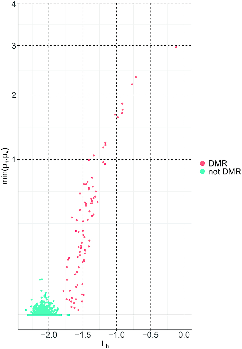
Bivariate plot of L_h (x-axis) and min (p_h, p) (y-axis). Each dot corresponds to a DNA region. The y-axis is square-root transformed to make is easier to see small values of min (p_h, p). The displayed observations were generated using the simulated dataset in the paper by Lee and Morris (16).

Figure 2.

A schematic overview of WS. The upper part of the figure represents the DNAm profiles of three randomly selected individuals for illustration purposes. The curved arrows represent the corresponding wavelet transformations. The bottom diagram represents the modeling of each wavelet coefficient. Each of these steps (1–4) is explained in greater detail in the main text.

Wavelet transformation and wavelet regression

WS tests for regional associations between a trait Ψ and a signal. We start here by describing step 1 in Figure 2. Suppose that we observe T CpG sites at base-pair positions bp_t, t = 1, ..., T in a given region for N individuals and that there is a positive integer J such that T = 2^J. Each individual’s DNAm profile in this region is treated as a signal, measured with an error. More precisely, M_{0, i}(bp) denotes the ‘true’ DNAm value of individual i at physical position bp (base pair), and M_i(bp) is the observed version of M_{0, i}(bp).

We assume that

(1)

where, for a fixed bp, the ε_i(bp) are independent and identically distributed over N individuals.

The wavelet transform performs local integrals to represent the DNAm profile. In principle, wavelet transform is analogous to Fourier transform, but instead of estimating the signal/function by performing global integrals, wavelet transform performs local integrals. Wavelet transform can thus identify signal modifications for different time points/locations and frequencies, which are commonly referred to as the time/frequency localization property of wavelet transform.

For a given region and individual i, we decompose the respective DNAm profile using Haar wavelet (simply referred to as wavelet transform in the rest of the paper). In essence, Haar wavelet estimates a function within an interval by generating local integrals at each step of the function (here, the DNAm profile). The integrals are called wavelet coefficients and are calculated for gradually smaller regions, half the size at each step. The wavelet coefficients are indexed using a two-digit code (s, l), where the first number, s, corresponds to the scale, while the second number, l, corresponds to the location. For example, (3,4) refers to the coefficient at the third scale, located at the step within the region.

The first step in the above calculation is an integration of the function over the entire selected region, which corresponds to the first wavelet coefficient, i.e. coefficient (0,0). The second step consists of calculating the integral twice: (i) over the first half of the interval (coefficient (1,1)) and (ii) over the second half of the interval (coefficient (1,2)). Thus, each subsequent step performs the integration over twice the number of intervals. Each of these steps defines a scale, which is also known as resolution or frequency. In our case, this process is repeated J times up to the scale J, given that our defined region has T CpGs, where T = 2^J.

In addition to the above time/frequency localization property, wavelet transform is an efficient signal-denoising tool. This is because smaller wavelet coefficients capture more of the noise in the measured function. Shrinking the small wavelet coefficients enables the removal of noise from the observed signal, a process known as wavelet shrinkage (17). In the current WS framework, we use the approach of Kovac and Silverman (40) to handle heteroscedastic noise in the wavelet shrinkage as well as to account for unevenly-spaced CpGs.

We now proceed with a description of step 2 in Figure 2. We first shrink each individual’s coefficients to obtain a set of wavelet coefficients based on the observed CpGs, which we call W_{s, l}. The scale s is between 1 and J, and the location l is between 1 and 2^s. We model the effect of each coefficient on the trait Ψ by reverse-regressing each wavelet coefficient. The model is

(2)

where C is a set of confounders, and ε is normally distributed noise with mean 0 and unknown variance. For conciseness, we dropped the individual index i in Equation (2). This model can handle either continuous or discrete traits. Lastly, as the shrunken wavelet coefficients are not normally distributed, we quantile-transform each wavelet coefficient across all the individuals, which reduces the number of false-positive findings due to distributional issues (41). To find all the β coefficients, we use Bayesian linear modeling with a Normal prior on (42), which gives the estimation . In practice, we use a vague prior, i.e. with a large standard deviation, centered at zero. Our software implementation also allows the use of the standard frequentist linear model.

Extracting summary statistics

In step 3 in Figure 2, we extract additional information from the estimations performed in step 2 and use it to build the test statistic in step 4. We model as being generated from two normal distributions, each representing the following hypotheses: and . We estimate the coefficients of the mixture model using an expectation-maximization (EM) algorithm (43). Then, using the coefficients of the mixture model, we compute the posterior probability of H₁ knowing , which is referred to as . We use the EM algorithm instead of the posterior distribution of to compute these posterior probabilities because the are not independent and tend to have the same sign when the scanned region is associated with the trait of interest (39). Thus, using the EM algorithm allows taking advantage of such clustering, whereas using individual posterior probability distributions would lower the estimation of the probability of .

As can be considered to be noisy wavelet coefficients, we shrink to reduce the noise from the estimation procedure. Rebuilding a signal using these coefficients would reconstruct an unscaled/dilated version of the proportion of association. As the quality of these estimates is a function of the sample size and the number of coefficients in the wavelet transform, we impose a thresholding approach that is a function of the sample size and the analysis scale. Similar to Donoho and Johnstone (44), we suggest the following thresholding:

(3)

Other thresholding approaches can also be used, such as those described by De Canditiis et al. (45) or Nason (17), but the above shrinkage is computationally fast and does not require any additional computation or modeling.

Next, we construct the two summary statistics that will subsequently be combined in step 4. The first summary statistic (L_h, see Equation 4) quantifies the degree of association between the trait and the wavelet coefficients.

(4)

(5)

Here, ϕ(x; μ, σ²) is the density of a normal distribution N(μ, σ²), with mean μ and variance σ² at the point x. The terms and correspond to the estimated parameters of the distribution of under the alternative hypothesis H₁, whereas the term corresponds to the estimated parameter of the distribution of under H₀. In our previous work (21), we suggested using the average of the weighted difference between the likelihood taken under H₁ and H₀ for each as a test statistic. In our current analyses, the weights are the estimated posterior probability of H₁ knowing and the estimated posterior probability of H₀ knowing , respectively.

We now construct the second summary statistic min (p, p_h) (see Equation 6) that quantifies the amount of grapes pattern. Following the works of Crouse et al. (38), Ma and Soriano (39) and our own (21), we assumed that, if a region is associated with Ψ, then the posterior probability of H₁ (i.e., ) exhibits a grapes pattern (see Figure 4). In other words, the associated would tend to be within the same region. Next, we extract two summary statistics, p_h and p, corresponding to the proportion of association per scale (i.e. horizontally) and subset (i.e. vertically), respectively.

(6)

(7)

(8)

In our previous work (21), we observed that the minimum of (p, p_h) is only marginally correlated with L_h under H₀ but exhibits a clear correlation with L_h when a region is associated with Ψ (see Figure 1). To increase the power for detecting a DMR, we take advantage of this difference in correlation between L_h and min (p, p_h).

Figure 4.

Region containing multiple subregions associated with OFCs. The differently colored rectangles highlight the regions with non-thresholded . The dots represent the estimated , with the size of a dot being proportional to its absolute value. Different colors are used to indicate the sign of (blue for negative, red for positive). close to zero are shown in white within a colored rectangle.

Combining the summary statistics

Finally, we build the combined test statistic (step 4 in Figure 2) using the above summary statistics and the hyperparameter λ (see Equation 9).

(9)

We select the hyperparameter λ via a data-driven procedure described in our original WS paper (21). In brief, we assume that L_h is normally distributed, and select a value of λ, denoted as λ*, that is as large as possible and that matches a fitting normal distribution criterion for . We then use this as a test statistic. We illustrate the result of this process in Figure 3. The distribution of for the ‘not differentially methylated region’ ‘not DMR’ remains close to the distribution of L_h for the ‘not DMR’, while the distribution of for the DMR shifts away from the null distribution.

Figure 3.

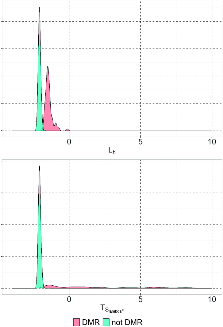
Distribution of the test statistic . The observations displayed here were generated using the simulated dataset from the Lee and Morris paper (16). The upper panel shows the distribution of L_h (λ = 0). The lower panel shows the distribution of (λ = 15).

We assess the significance of each regional test statistic () by simulating it under H₀. This can easily be done using the null distribution of (for additional details, see page two of the Supplementary Data in Servin and Stephens (46)). Simulating a million observations of under H₀ can be executed in <5 min on an ordinary laptop.

Handling low-scale regions

L _h tends to be normally distributed within the high-scale regions (scale ≥6). Therefore, the normality assumption can be used when analyzing large regions that are more densely populated with observations, as would be the case with an imputed GWAS dataset containing over 8 million SNPs, a high-density DNAm dataset generated on the CHARM platform (47), or data generated using whole-genome bisulphite sequencing (WGBS). However, most DNAm datasets tend to have low probe density, especially those emanating from array-based measurements. Under such conditions, the scale of our analysis would be low a priori (e.g. below 5), and the L_h statistics may not be normally distributed because only a few coefficients would be available to compute this average. For instance, a scale of 3 corresponds to only 16 coefficients, a scale of 8 to 512 coefficients, a scale of 9 to 1024 coefficients, and so forth.

To handle the issue of non-normality, we apply a Box-Cox transform (48) to the −L_h statistics, based on the empirical observation that L_h is negative. We simulate L_h 10⁶ times under H₀ and use the simulated value to optimize the choice of λ_BC, which is the parameter of the Box-Cox transform on −L_h. We select the that maximizes the likelihood function and transform the observed l_h (called and , respectively) using the transformation . Finally, we apply the procedure described in the previous subsection on ‘Combining the summary statistics’ to the equation below:

(10)

When we applied the above method to our OFCs DNAm dataset, the simulations yielded and λ* = 26. These values were subsequently used to assess the significance of each region. Supplementary Figures S1 and S2 confirm that the transformed test statistic has a good fit.

Post-processing of the WS output

Mapping procedure for subregions

Although most of the associations detected by WS covered an entire region, a few of the associations only covered a region partially. We call such partially associated regions ‘subregions’. One may detect a subregion when analyzing larger regions that are more likely to contain several distinctly associated subregions, as illustrated in Figure 4. For downstream analyses, we focus on subregions that showed an association with OFCs (see the subsection below on ‘Procedure for selecting DNAm regions’). We thus implement the following mapping strategy in our WS R package: for each associated region, we select the with a non-thresholded posterior probability of belonging to H₁ (). These correspond to the overlaid regions (highlighted as colored rectangles in Figure 4). We then extract the coordinates of the associated subregions that contribute to the wavelet coefficient s, l, using the mapping function in our WS R package.

GSEA in combination with an over-representation analysis

GSEA is a widely used computational tool for analyzing the output of a genetic association study (49–51). It can be used to determine whether an a priori defined set of genes shows statistically significant and concordant differences between two biological states (for further details on the method, see the paper by Subramanian et al. (52) and http://software.broadinstitute.org/gsea/index.jsp).

For a given set of genes G of length l, and for each item in the Molecular Signatures Database (MSigDB) of annotated gene sets for the GSEA, the over-representation analysis compares the number of genes in G that are annotated with a specific term to the expected number of genes annotated with this term if l genes were selected at random from the entire genome. Figure 7 explains the rationale behind the overrepresentation analysis. The P-values for each gene annotation are obtained using Fisher’s exact test for hypergeometric distributions. Owing to its simplicity and robustness compared to other methods for GSEA, we used the online-based GSEA platform, WebGestalt (50), to query a large list of gene-annotation databases simultaneously and to perform an over-representation analysis in each of these databases. It is well-documented that a GSEA may be biased due to differences in the number of CpG sites associated with different classes of genes and gene promoters (15). However, since they require a P-value for each CpG, the published implementations of unbiased GSEAs for DNAm (e.g. (51,53)) cannot be applied directly to the output of WS.

Figure 7.

Schematic overview of the over-representation analysis. The left panel displays the expected overlap between a set of annotated genes and the genes associated with OFCs. The right panel displays an over-represented annotated set of genes for OFCs.

APPLICATION OF WAVELET SCREENING

OFCs dataset

The main dataset for the current analyses comes from the Norway Facial Cleft Study (36), a large Norwegian population-based case–control study of OFCs comprising 750 cases and 1100 controls. DNAm data were only available on a subset of the infants (418 OFCs cases and 480 controls). The OFCs cases comprised 167 cases with cleft lip and cleft palate (CLP), 144 cases with cleft palate only (CPO) and 107 cases with cleft lip only (CLO) (14). DNAm was measured on the Illumina 450K platform using DNA derived from heel-prick blood samples from the infants. Information on known confounders was collected via self-administered questionnaires (36).

The criteria for quality control have been described in the original EWAS by Xu et al. (14). Briefly, low-quality methylation data were filtered out using Illumina’s bisulphite internal control, and probes with > low-quality data were excluded (Illumina detection P-values ≤10⁻⁶, n = 23 264 CpGs). Probe outliers and samples with ambiguous sex were also removed. To avoid confounding of effects by common SNPs, 53 247 CpGs that had a neighboring SNP with a minor allele frequency ≥0.05 (for a European population) were removed. Finally, n = 1488 CpGs with multimodal DNAm level distributions were removed using the ENmix R package (54). The data were also corrected for sex and plate number.

After the above quality control, 868 individuals (456 controls and 412 OFCs cases (i.e. 167 CLP, 140 CPO and 105 CLO)) and 407 513 CpGs from the original 497 513 CpGs were left for the current analyses. We focused only on the autosomes and analyzed all three cleft subtypes together (n = 412) against the controls.

Procedure for selecting DNAm regions

In their investigation, Jenkinson et al. (8) considered 3 kb-long stretches of DNA containing at least 10 CpGs. In the worst-case scenario, this would result in an average distance of 500 bp between any two adjacent CpGs. We use a similar criterion and analyze regions containing at least 9 CpGs separated by a maximum distance of 500 bp. We choose 9 instead of 10 CpGs for practical reasons. First, this leads to the inclusion of more CpGs in our analyses. Second, in order to use the interpolation scheme of Kovac and Silverman (40) for analyzing unevenly-spaced signals at scale J, one needs to have at least 2^J + 1 observations. Using a scale of 3 (i.e. J = 3) would entail having at least 2³ + 1 = 9 CpGs per analyzed region.

Figure 5 provides a schematic overview of the procedure for selecting DNAm regions. In contrast to all the previously mentioned methods and analytic approaches, we do not analyze regions of a fixed size but instead consider regions of variable sizes (see Figure 6).

Figure 5.

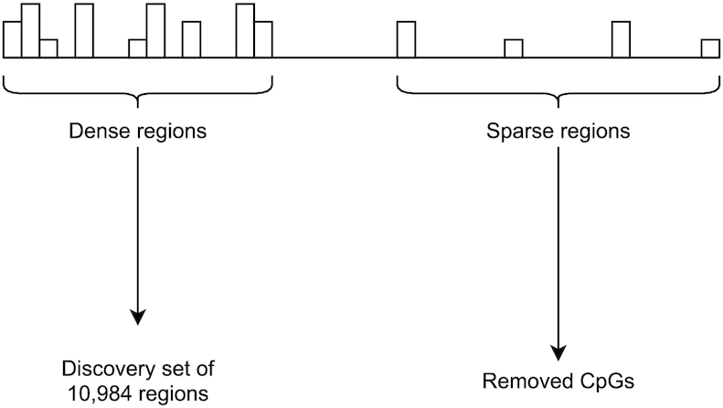
Overview of the selection of DNAm regions.

Figure 6.

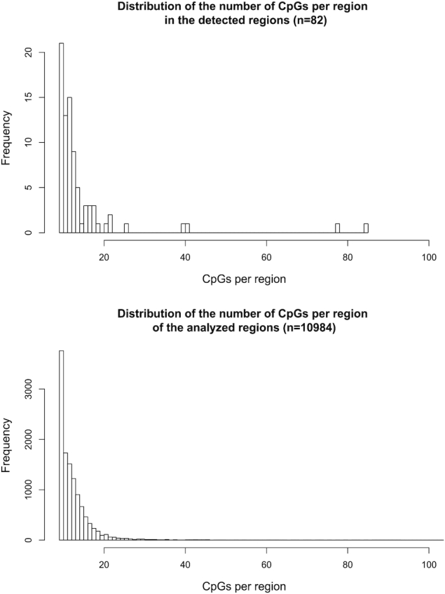
Distribution of the number of CpGs per region for the 82 associated regions (upper panel) and for a total of 10 984 analyzed regions (the discovery set; lower panel).

The 407 513 CpGs remaining after the original 497 513 CpGs were subjected to quality control and were subsequently used to define DNAm regions according to the two main criteria mentioned above: (i) a given region must contain at least 9 CpGs and (ii) any pair of adjacent CpGs must not be separated by >500 bp. This resulted in a total of 10 984 distinct regions, which we refer to as our discovery set. Collectively, these regions represent approximately of the assayed CpGs on the Illumina 450K platform.

Based on the rationale above, we use a scale of 3 to analyze each region. Applying a Bonferroni correction leads to a significance level of for the 10 984 above-defined regions. In the Results section, we describe the outcome of this analysis and provide further details regarding the regions detected by WS.

Permutation

We perform permutations for each run of WS to demonstrate its reliability. The observed trait (here, OFCs) and the CpG sites are used to estimate the proportion of false positives per run. An EWAS is first performed using a permuted phenotype to assess the type I error, and the P-value for each region (for the permuted phenotype) is subsequently computed. The proportion of P-values below the Bonferroni threshold of 4.5 × 10⁻⁶ provides an empirical estimate of the proportion of false positives per run. The above permutation is repeated 100 times to obtain a reliable estimate of the proportion of false positives.

Simulated dataset

To further investigate the power of WS, we applied it to a simulated dataset that can be found at http://odin.mdacc.tmc.edu/∼jmorris/simulated_data.Rdata. This dataset was generated on the CHARM platform (47) and consists of 26 methylation profiles on chromosome 3 containing a total of 75 069 probes. The phenotype (Ψ) is a binary indicator corresponding to either a cancer cell (Ψ = 1) or a control cell (Ψ = 0). The simulations are designed to ensure that the two groups have the same DNAm profile for all CpGs, except for the 1901 loci reported to be differentially methylated in Irizarry et al. (6). More details on the simulated dataset can be found in the Supplementary Data of the paper by Lee and Morris (16).

As explained in the subsection ‘Procedure for selecting DNAm regions’, we divided the DNAm profile into regions. To evaluate the performance of WS on denser platforms, we used a stricter criterion to divide the region, i.e. each region must contain at least 17 CpGs (1 + 2⁴), with any two adjacent CpGs separated by a maximum distance of 500 bp. This pre-processing resulted in a total of 1213 regions, which included 1875 of the 1901 loci reported by Irizarry and colleagues (6), distributed between 89 of the 1213 defined regions. For each region, we investigated whether the CpG patterns varied in the cancer (n = 13) versus control (n = 13) cells. As each region contains at least 17 CpGs, we used a depth of analysis of 4. The script for these analyses is provided in the Supplementary Data.

To contrast the performance of WS against other popular software for DMR detection, we analyzed the 1213 defined regions using Bumphunter (3) and ‘Wavelet-based Functional Mixed Models’ (WFMM) (16,18). Note that a comparison with DMRcate (11) was not possible because the implementation of DMRcate does not support the analysis of data from the CHARM array. WFMM is a wavelet-based functional modeling that can be used to detect DMRs (16). It uses an empirical Bayes approach to perform a regularization of the estimated effect, and the modeling can take into account a large range of correlations between the observed DNAm profiles. WFMM can thus handle repeated measures of DNAm.

When applied to the simulated dataset of repeated measurements available at http://odin.mdacc.tmc.edu/∼jmorris/simulated_data.Rdata, WFMM processed all 75 069 CpG sites in one go and computed the posterior probability of each CpG site being above a set threshold (here 0.1 and 0.05) for being associated with cancer. As the data are measured twice on each patient (once in control cells and once in cancer cells), we ran WFMM by specifying the correlation structure between paired observations. Next, following the approach by Lee and Morris (16), we transformed the posterior probabilities of the CpGs into Bayesian FDR values (16).

Furthermore, in order to compare WFMM with WS, we first needed to assign a regional significance criterion for WFMM. To do this, we used the minimum Bayesian FDR value for all the CpGs within a region of interest. After running WFMM on the entire dataset, we used the minimum Bayesian FDR values for each of these regions as a measure of significance.

Like WFMM, Bumphunter (3) can also be used to detect a DMR based on a given threshold. However, unlike WFMM, Bumphunter starts by estimating the effect of cancer on the methylation level at each CpG site and then smooths the estimated effects using ‘locally estimated scatterplot smoothing’ (Loess) (55). If the smoothed effects contain several adjacent CpGs that have an effect above the set threshold, Bumphunter declares this set of CpGs as being a DMR. Finally, the significance of each DMR was assessed using a permutation procedure. Bumphunter was run using the same threshold as for WFMM (0.1 and 0.05). We used the Bumphunter implementation in the Minfi package (56), which requires re-running the method for each considered threshold. Similarly, as with WFMM, we used each DMR p-value to compute its corresponding FDR.

Finally, for each method and threshold, we saved the actual running time as a measure of efficiency. All the computations were performed on a laptop equipped with an Intel(R) i7-700HQ 2.80 GHz processor and 8 GB of RAM.

RESULTS

Testing the power of WS using a simulated dataset

Despite the application of a more stringent criterion to define the regions of the discovery set on the CHARM platform, we still managed to analyze of the available CpGs. This is a substantial increase in coverage compared to the sparser platforms (450K and EPIC 850K). We detected 90 regions with a P-value below 10⁻⁵ (Bonferroni-corrected for 1000 tests) out of the regions that contained all the differentially methylated CpGs. These 90 regions contained two false positives. Similarly, we detected 86 out of the 89 regions with a P-value below 10⁻⁶, which, again, contained two false positives (Bonferroni-corrected for 10 000 tests). This corresponds to a power of and , respectively.

When using a false-discovery rate (FDR) of 0.01, we detected 92 associated regions. These 92 regions contained three false positives. By contrast, we detected 95 regions with an FDR = 0.05. Those regions contained the 89 truly associated regions and six false-positive regions (this corresponds to a false discovery proportion of , which is close to the expected proportion of false discovery ()).

Table 1 summarizes the results of the analyses by WS, WFMM, and Bumphunter. Overall, WS is significantly faster than WFMM and Bumphunter, and has higher power for detecting DMRs. The results of the analysis by WS contain a few more false positives than those by WFMM and Bumphunter. However, the number of false discoveries with WS remains in the range of expected false discoveries at each nominal level of FDR. Assessing power is easier with WS, as this does not need a predefined threshold for detecting DMRs. By contrast, WFMM and Bumphunter search for DMRs at a given threshold, and their power can therefore only be evaluated at a given threshold. The thresholds we used (0.05 and 0.1) are somewhat conservative, especially when compared to the standard threshold of 0.25 used in the Minfi package (56) for Bumphunter.

Table 1.

Number of regions detected by WS, WFMM, and Bumphunter according to different correction criteria. NA: not applicable

Method	Threshold	FDR	Number	Number	Run
		level	of detected	of true	time (s)
			regions	regions
WS	NA		95	89	61
WS	NA		92	89	61
WFMM	0.1		86	86	23 521
WFMM	0.1		77	77	23 521
WFMM	0.05		89	89	23 521
WFMM	0.05		89	89	23 521
BH	0.1		64	64	3 948
BH	0.1		64	64	3 948
BH	0.05		86	85	11 449
BH	0.05		86	85	11 449

Taken together, the high coverage of the analysis ( of the CpGs) coupled with the high power ( with an FDR = 0.01) demonstrate the versatility and robustness of WS for denser platforms. We provide a script in the Supplementary Data to allow other researchers to reproduce the results of our analysis here based on the simulated dataset by Lee and Morris (16).

Applying WS to a DNAm dataset of OFCs

We used WS to screen for associations between DNAm profiles and OFCs, and conducted additional analyses to assess the reliability of the method. The permutations showed that 94 regions were below the Bonferroni threshold of 4.5 × 10⁻⁶, which corresponds to one false discovery per run. In addition, the calibration of the test statistic confirmed that there was a good fit, as indicated by the normal Q-Q plot of the observed test statistics in Supplementary Figures S1 and S2.

Based on this calibration, 82 regions were found to be associated with OFCs. These regions are highlighted in bold in Supplementary Table S2. Even though a variable region size was used to analyze the selected regions, WS did not appear to be biased towards any specific region size. Figure 6 shows that the distribution of the discovery set (10 984 regions) was similar to that of the associated regions (Kolmogorov–Smirnoff test P-value =0.53). Furthermore, WS did not appear to be biased towards any specific type of CpG site (CpG island, shore or open sea).

We applied the mapping procedure outlined in the subsection ‘Post-processing of the WS output’ to the 82 regions found to be associated with OFCs, and identified a further 120 associated subregions. We specified the coordinates of the subregions in the UCSC Table Browser (57) (http://genome.ucsc.edu) to determine whether the subregions contained any genes. This led to the identification of 84 genes within the subregions (Supplementary Table S2). To explore the relevance of these genes, we used WebGestalt (50) to perform GSEA. A total of 84 genes were enriched for 53 traits/biological processes at an FDR below , and 166 traits/biological processes were enriched at an FDR below (Supplementary Table S1).

The list of genes and loci showing an association with OFCs and other craniofacial anomalies is provided in Supplementary Table S2. Strikingly, WS found associations with several genes previously implicated in OFCs and other craniofacial anomalies (highlighted in bold in Supplementary Table S2 and described in more detail in Table 2). In addition, our GSEA revealed several biological processes known to be involved in the morphogenesis of craniofacial features. These include ‘positive regulation of cellular biosynthetic processes’ (), ‘negative regulation of developmental processes’ (), ‘regulation of cell migration’ () and ‘regulation of cell differentiation’ () (see also Supplementary Table S1). Furthermore, in line with the critical roles played by cellular adhesion and junction organization in the spatio-temporal fusion of the primary and secondary palates, GSEA identified a link with ‘regulation of cell adhesion’ (), ‘regulation of cell junction assembly’ (), ‘cell junction assembly’ (), and ‘adherents junction organization’ (). It also identified several abnormalities associated with OFCs (58–60), including ‘congenital malformation of the left heart’ (), ‘smooth philtrum’ (), ‘abnormality of dental morphology’ (), ‘abnormality of the dental root’ (), and ‘abnormality of brain morphology’ ().

Table 2.

Genes identified by WS that have previously been linked with OFCs and craniofacial anomalies

Gene symbol	Comments	Reference(s)
ATP6V0A2	Connected to OFCs via a study of a consanguineous family afflicted with the rare congenital disorder Autosomal recessive Cutis laxa type IIA (ARCL2A). Two of the affected individuals in this family had cleft lip and palate along with several other clinical features.	(71)
CBFB	Encodes a co-factor of the RUNX family of transcription factors and is part of the RUNX1/CBFB-STAT3-TGFB3 signaling axis. Both RUNX1 and TGFB3 are known to play central roles in the fusion of the primary and secondary palatal shelves. In humans, haploinsufficiency for CBFB results in cleft palate, among several other clinical manifestations (72), and, in mice, a nonfunctional Cbfb disrupts the formation of the anterior palate.	(72,73)
DRD2	Encodes the D2 subtype of the dopamine receptor. The combination of a specific DRD2 polymorphism (the Taq1 A1 allele) and OFCs is associated with fewer inattentive ADHD symptoms.	(74)
EVC, MSX1 and STK32B	Located in the 4p16 locus. MSX1, EVC and STK32B have been associated with OFCs, which suggests that several genes at the 4p16 locus might be influencing the risk of OFCs. MSX1 has long been recognized as a major gene for OFCs. For example, knocking out MSX1 in mice causes a complete cleft of the secondary palate and several other craniofacial defects. Furthermore, a nonsense mutation in MSX1 in a Dutch family was found to segregate with tooth agenesis and mixed clefting, pointing to an important role for MSX1 in normal facial morphogenesis.	(75–78)
F3	Identified by investigating DNAm and genetic influences on the liability to isolated CL/P. Despite an extensive literature search, however, we were unable to find other connections between F3 and OFCs. It would, nevertheless, be premature to discard this gene as a false positive until other independent OFCs cohorts have run their EWASes and are able to provide a more definitive answer.	(34)
LDB1	Transcription co-factor. Almaidhan and co-workers demonstrated that Ldb1 is essential for normal development of the secondary palate in mouse embryos. This gene is involved in pathways that mediate epithelial–mesenchymal interactions during palatogenesis.	(79,80)
SENP2	Involved in a post-translational modification called sumoylation, which has a well-documented function in palatogenesis. A patient with isolated CLP had a balanced reciprocal translocation resulting in haploinsufficiency for SUMO1. The protein product of this gene belongs to the small ubiquitin-like modifier (SUMO) protein family. Mice carrying a Sumo1-hypomorphic allele were reported to develop cleft palate.	(81,82)
SHOX2	Belongs to the homeobox family of genes. There is a large body of evidence demonstrating an intrinsic requirement for SHOX2 in normal palatogenesis. In humans, mutations in SHOX2 are associated with idiopathic short stature. Shox2 deficiency in mice results in the development of an incomplete cleft affecting the anterior (hard) region of the palate.	(83–89)
SYT14	Member of the synaptotagmin gene family. Among a multitude of functions, synaptotagmins regulate the release of neurotransmitters stored in synaptic vesicles in response to a rise in the level of intracellular calcium. Mutations in SYT14 have been linked to several human neurodegenerative disorders. A GWAS of 144 cleft palate trios from a Western Han Chinese population showed evidence of a gene-by-gene interaction between a SNP in SYT14, and another SNP located 37 kb from the gene ‘UTP25 small subunit processor component’ (UTP25).	(90)
TBX5	Belongs to the T-box gene family containing a DNA-binding motif called the T-box domain that binds to DNA in a sequence-specific manner. Several members of this gene family have a well-established role in human developmental syndromes. For example, mutations in TBX22 cause a syndromic form of clefting known as ‘X-linked cleft palate with or without ankyloglossia’ (CPX). Ak-Qattan et al. reported a novel missense mutation in TBX5 in a Saudi infant with Holt–Oram syndrome. In a more recent study of a Chinese population of isolated CL/P trios, a gene-by-gene interaction was reported between a SNP in TBX5 and another SNP in ‘fibroblast growth factor 10’ (FGF10). The connection between TBX5 and FGF10 is particularly noteworthy given previous evidence of a strong association between isolated CL/P and a common genetic variant in FGF10, as well as the importance of the FGF10–FGFR2 pathway in human orofacial development.	(91–93)
WDR19 (alias IFT144)	Mutations in genes comprising the IFT machinery, of which IFT144 is a key component, underlie a pleiotropic group of diseases and syndromic disorders known as ciliopathies. Cilia are motile hairlike structures on the surface of eukaryotic cells that enable the cells to move around through fluids. Consistent with the phenotypes in humans, mutations in Ift144 lead to several phenotypes in mice that closely resemble the skeletal and craniofacial anomalies observed in patients with ciliopathies.	(94)
NPAT/ATM	Identified by investigating genotypic differences between cases with non-syndromic CL/P and controls in a Polish cohort.	(95)

DISCUSSION

This paper presents a fast and powerful wavelet-based approach for analyzing DNAm data from different platforms, irrespective of their probe density. To showcase the utility of WS, we applied it to the largest EWAS dataset of OFCs to date. Only a handful of studies have investigated CpGs in the context of OFCs (13,14,34,61,62), and they were either based on single-CpG modeling or regional tests using the software Comb-p (12) or Bumphunter (3). Furthermore, they were limited by the relatively small sample sizes (typically, 50–70 OFCs cases) and the lack of statistical power and flexibility of the methods in handling more complex DNAm profiles. The high coverage of the analysis with WS ( of the CpG sites) coupled with its high power ( with an FDR = 0.01) demonstrate the robustness of WS for denser platforms.

The enhanced flexibility and statistical power of WS in modeling different types of omics data is an important step forward in addressing the issue of missing heritability in OFCs and other complex traits (63). Although WS does not provide any direct estimates of heritability, its downstream analyses, such as the GSEA and the accompanying over-representation analysis, may assist in identifying genes that might have been overlooked by conventional methods. This makes WS a particularly versatile and attractive tool for an initial screening of a given DNAm dataset in order to uncover additional genes and loci that are associated with the trait.

GSEA analysis

Our GSEA of the OFCs dataset revealed several key biological processes known to be involved in the morphogenesis of craniofacial features. These include the regulation of developmental processes, cell migration, cellular differentiation and cellular adhesion (64–66). Non-isolated (syndromic) OFCs are accompanied by other abnormalities, including congenital heart defects, hypodontia and other dental anomalies, and abnormal brain morphology, among others (58–60). Our OFCs sample included non-isolated cases to enable an exploration of comorbidities that might share a common genetic background with isolated clefts. Hence, it is not surprising to observe an enrichment for several congenital malformations in our gene set of 84 genes.

In particular, the links between OFCs and dental anomalies are noteworthy, given the known connections between these phenotypes (67–69). Furthermore, in line with the results of a recent Mendelian randomization analysis by Howe et al. (61), our GSEA also showed an enrichment for the phenotype ‘smooth philtrum’ (FDR = 0.0416), further supporting the hypothesis that OFCs and the philtrum share a common genetic pathway owing to their physical proximity (70).

Genes identified by WS in OFCs

Identifying 11 genes that have previously been linked with OFCs and other craniofacial anomalies (Table 2), either directly or indirectly through their involvement in key molecular circuits regulating craniofacial development, underscores the robustness and validity of WS. These connections also point to the potential involvement of a large number of genes acting in concert to orchestrate the many delicate processes that contribute to the morphogenesis of the human face (70). It would thus be premature to dismiss the veracity of the remaining genes and loci displayed in Supplementary Table S2 merely on the basis of the absence of a published link with OFCs in the literature. We have thus opted to publish the entire list of genes and loci detected by WS to enable other OFCs researchers to contrast their findings with ours after having run their analyses using WS (or a comparable method).

Comparison with previous studies

A previous analysis of the same OFCs dataset consisted of three separate epigenome-wide analyses (14). The first was a logistic regression carried out on each CpG, while the other analyses were regional tests conducted using the software DMRcate (11) and Comb-p (12). Xu et al. (14) defined a DMR as a region containing at least two CpGs separated by ≤1 kb, with a Šidák multiple testing-corrected P-value of <0.05. They used a fixed window size of 1 kb in both the DMRcate and Comb-p analyses. Compared to our approach, however, they only considered regions of a fixed size and did not take CpG density into account. Their analyses detected only two significant differentially methylated CpGs, one with CL/P and the other when CPO was combined with CLP. No DMRs were detected by DMRcate for any of the cleft subtypes, but 37 DMRs were detected by Comb-p when all the cleft subtypes were analyzed together. In the DMRs detected by Comb-p, only five had >9 CpGs (one on chromosome 1 and four on chromosome 6). Even though these DMRs were not present in our discovery set, WS nonetheless detected four associated regions on chromosome 6 that are near the DMRs detected by Xu et al. (14) and Phan et al. (68) (see Supplementary Table S2 for more details).

Our discovery set did not overlap with the 11 methylation variable positions (MVPs) reported by Alvizi et al. (62). In that paper, the authors performed an EWAS of CLP cases versus controls in a Brazilian OFCs sample and selected eleven of the top MVPs from a total of 578 detected MVPs for replication in a British cohort. Only three of the 578 MVPs from the Brazilian study overlapped with our discovery set. These contained the CpGs cg07949612, cg21284370 and cg26420824, located in the genes ‘NFU1 iron-sulfur cluster scaffold’ (NFU1), ‘Diacylglycerol kinase eta’ (DGKH) and ‘ATP synthase inhibitory factor subunit 1’ (ATP5IF1), respectively. The lack of overlap in findings could be attributed to the relatively small sample size of the Brazilian discovery sample (68 cases and 59 controls) compared to ours. Moreover, the authors specifically studied CpGs related to CLP alone, and not to the combined sample of all the OFCs subtypes.

Similar to the Brazilian study, our results showed little overlap with those of Howe et al. (34), except for the Coagulation factor III, tissue factor (F3) gene. Howe et al. investigated whether genetic risk variants influenced DNAm associated with all the OFCs subtypes combined versus controls. Several scenarios were investigated using Mendelian randomization to explore which CpGs were associated with the combined sample of all the OFCs subtypes versus the controls. In all the considered scenarios, Howe et al. first performed a ‘forward selection’. In this first step, 21 CpGs were found to be associated with the combined sample of all OFCs subtypes. In particular, an association was detected with cg09549015 located in F3. However, when Howe et al. investigated more complex causal scenarios based on the forward selection, the association with F3 disappeared. As already mentioned, F3 also showed up in our discovery set.

Methodological considerations

We opted to showcase our method by applying it to the combined sample of all three cleft subtypes. However, cases with isolated OFCs, i.e. those without any accompanying congenital anomalies, are routinely split into three main subtypes: CLO, CLP and CPO, with CLP often collapsed with CLO to form the cleft lip with or without cleft palate (CL/P) category. We analyzed all the cleft subtypes together, but a more comprehensive application to each subtype separately could potentially unravel additional insights into the genetic heterogeneity across these cleft subtypes, especially when a large enough sample size has accrued to allow such subanalyses with adequate power.

Another important methodological consideration is that our regional test models the effect of the DNAm profile for a given region directly. This differs from previous approaches to regional modeling of DNAm data, where single-CpG associations were processed into a regional test (3,5,11,12,16). WS initially decomposes the individual regional DNAm pattern into wavelet coefficients (i.e. into a functional representation of the DNAm profile) and then uses these coefficients to perform the regional test. Compared to the approach by Morris and Carroll (18), we model the effect of each wavelet coefficient independently, which results in higher computational efficiency because a sampling algorithm such as MCMC is no longer required. Thus, WS has a markedly lower computational burden than traditional methods for EWAS, and it is possible to perform a full genome-wide analysis of 1000s of individuals on a single CPU in a matter of 2−3 h.

Another major advantage of WS is that it allows the use of principal components to adjust for population stratification and other confounding factors. Given that WS does not require a preassigned threshold (as is, for example, the case with Bumphunter (3) and WFMM (16)), it enables a more straightforward comparison of results across studies. When using the simulated dataset from the study by Lee and Morris (16), WS showed higher power and was significantly faster than both Bumphunter and WFMM. The large difference in run time between the three methods can be explained by the different procedures used by each method to assess the significance of a DMR (i.e. bootstrap by Bumphunter, MCMC by WFMM, and Monte-Carlo by WS).

• Bumphunter tests for systematic differences in DNAm profiles between cases and controls. When Bumphunter detects a difference larger than a set threshold between cases and controls, it evaluates its significance using a bootstrapping procedure. Therefore, Bumphunter performs a bootstrap for each potential DMR. As the number of potential DMRs increases when the threshold is lowered, the run time of Bumphunter increases accordingly. Table 1 illustrates this phenomenon.

• WFMM estimates the change in DNAm profile between cases and controls along the entire genome using a wavelet-based approach that requires the use of MCMC. WFMM then uses the draws from the posterior distribution of the change in DNAm profile to detect a DMR. The MCMC in WFMM carries most of the computational burden.

• WS computes regression coefficients between the wavelet-transformed DNAm profile and then applies an EM algorithm to detect clusters of associations. The main advantage of WS is that the test statistics of all the screened regions () have the same null distribution and can thus be simulated quickly. Hence, WS only needs to simulate the null distribution once, as opposed to Bumphunter where each potential DMR has a different null distribution that needs to be simulated separately.

Finally, the analysis coverage of WS increased to with data from the CHARM platform. The current Illumina EPIC platform contains approximately 850K CpG sites, which is almost twice the number of probes than the former 450K platform. If the next generation of DNAm platform doubles the number of interrogated CpG sites, its density will increase to a level similar to that of the CHARM platform, which means that WS would be able to analyze a similar percentage of CpG sites (roughly ). In addition, the recent introduction to whole-genome bisulfite sequencing (WGBS, see the application note at https://www.illumina.com/) at reduced cost (96) will contribute to substantially larger EWASes and thereby higher power for WS analyses.

CONCLUSION

We analyzed a discovery set of 10 984 DNAm regions covering approximately of the CpGs on the 450K platform and used extensive simulations to demonstrate the robustness and reliability of WS. The percentage of CpGs covered is expected to rise with the application of significantly denser platforms, such as the EPIC 850K and CHARM. Our analyses of the OFCs dataset identified 82 associated regions containing a large number of genes and loci previously reported to influence the risk of OFCs, while others are novel and await replication in other cohorts. Although our primary focus was on EWAS, WS is highly versatile and easily amenable to the analysis of other types of omics data. It has now become relatively straightforward to gain access to the results of a large number of publicly available EWASes through various data repositories around the world (e.g. the GEO database (97)). We thus envisage WS to become an attractive tool for re-analyzing these datasets, enabling the discovery of additional genes and loci that might have been missed by previous efforts.

SUPPLEMENTARY DATA

Supplementary Data are available at NARGAB Online.

FUNDING

Research Council of Norway (RCN) [249779 (in part)]; Bergen Medical Research Foundation (BMFS) [807191]; RCN [262700].

Conflict of interest statement. None declared.

REFERENCES

- 1. Yong W.-S., Hsu F.-M., Chen P.-Y.. Profiling genome-wide DNA methylation. Epigenet. Chromatin. 2016; 9:26. [DOI] [PMC free article] [PubMed] [Google Scholar]
- 2. Lovkvist C., Dodd I. B., Sneppen K., Haerter J. O.. DNA methylation in human epigenomes depends on local topology of CpG sites. Nucleic Acids Res. 2016; 44:5123–5132. [DOI] [PMC free article] [PubMed] [Google Scholar]
- 3. Jaffe A.E., Murakami P., Lee H., Leek J.T., Fallin M.D., Feinberg A.P., Irizarry R.A.. Bump hunting to identify differentially methylated regions in epigenetic epidemiology studies. Int. J. Epidemiol. 2012; 41:200–209. [DOI] [PMC free article] [PubMed] [Google Scholar]
- 4. Lunnon K., Smith R., Hannon E., De Jager P.L., Srivastava G., Volta M., Troakes C., Al-Sarraj S., Burrage J., Macdonald R.et al.. Methylomic profiling implicates cortical deregulation of ANK1 in Alzheimer’s disease. Nat. Neurosci. 2014; 17:1164–1170. [DOI] [PMC free article] [PubMed] [Google Scholar]
- 5. Martorell-Marugán J., González-Rumayor V., Carmona-Sáez P.. mCSEA: detecting subtle differentially methylated regions. Bioinformatics. 2019; 35:3257–3262. [DOI] [PubMed] [Google Scholar]
- 6. Irizarry R.A., Ladd-Acosta C., Wen B., Wu Z., Montano C., Onyango P., Cui H., Gabo K., Rongione M., Webster M.et al.. The human colon cancer methylome shows similar hypo- and hypermethylation at conserved tissue-specific CpG island shores. Nat. Genet. 2009; 41:178–186. [DOI] [PMC free article] [PubMed] [Google Scholar]
- 7. Laird P.W. Principles and challenges of genome-wide DNA methylation analysis. Nat. Rev. Genet. 2010; 11:191–203. [DOI] [PubMed] [Google Scholar]
- 8. Jenkinson G., Pujadas E., Goutsias J., Feinberg A.P.. Potential energy landscapes identify the information-theoretic nature of the epigenome. Nat. Genet. 2017; 49:719–729. [DOI] [PMC free article] [PubMed] [Google Scholar]
- 9. Szabo Q., Bantignies F., Cavalli G.. Principles of genome folding into topologically associating domains. Sci. Adv. 2019; 5:eaaw1668. [DOI] [PMC free article] [PubMed] [Google Scholar]
- 10. Pombo A., Dillon N.. Three-dimensional genome architecture: players and mechanisms. Nat. Rev. Mol. Cell Biol. 2015; 16:245–257. [DOI] [PubMed] [Google Scholar]
- 11. Peters T.J., Buckley M.J., Statham A.L., Pidsley R., Samaras K., V Lord R., Clark S.J., Molloy P.L.. De novo identification of differentially methylated regions in the human genome. Epigenet. Chromatin. 2015; 8:6. [DOI] [PMC free article] [PubMed] [Google Scholar]
- 12. Pedersen B.S., Schwartz D.A., Yang I.V., Kechris K.J.. Comb-p: software for combining, analyzing, grouping and correcting spatially correlated P-values. Bioinformatics. 2012; 28:2986–2988. [DOI] [PMC free article] [PubMed] [Google Scholar]
- 13. Sharp G.C., Ho K., Davies A., Stergiakouli E., Humphries K., McArdle W., Sandy J., Davey Smith G., Lewis S.J., Relton C.L.. Distinct DNA methylation profiles in subtypes of orofacial cleft. Clin. Epigenetics. 2017; 9:63. [DOI] [PMC free article] [PubMed] [Google Scholar]
- 14. Xu Z., Lie R.T., Wilcox A.J., Saugstad O.D., Taylor J.A.. A comparison of DNA methylation in newborn blood samples from infants with and without orofacial clefts. Clin. Epigenetics. 2019; 11:40. [DOI] [PMC free article] [PubMed] [Google Scholar]
- 15. Geeleher P., Hartnett L., Egan L.J., Golden A., Raja Ali R.A., Seoighe C.. Gene-set analysis is severely biased when applied to genome-wide methylation data. Bioinformatics (England). 2013; 29:1851–1857. [DOI] [PubMed] [Google Scholar]
- 16. Lee W., Morris J.S.. Identification of differentially methylated loci using wavelet-based functional mixed models. Bioinformatics. 2016; 32:664–672. [DOI] [PMC free article] [PubMed] [Google Scholar]
- 17. Nason G. Wavelet Methods in Statistics with R, Use R!. 2008; New York: Springer-Verlag. [Google Scholar]
- 18. Morris J.S., Carroll R.J.. Wavelet-based functional mixed models. J. R. Stat. Soc. Series B (Stat. Methodol.). 2006; 68:179–199. [DOI] [PMC free article] [PubMed] [Google Scholar]
- 19. Shim H., Stephens M.. Wavelet-based genetic association analysis of functional phenotypes arising from high-throughput sequencing assays. Ann. Appl. Stat. 2015; 9:665–686. [DOI] [PMC free article] [PubMed] [Google Scholar]
- 20. Vsevolozhskaya O.A., Zaykin D.V., Greenwood M.C., Wei C., Lu Q.. Functional analysis of variance for association studies. PLOS ONE. 2014; 9:e105074. [DOI] [PMC free article] [PubMed] [Google Scholar]
- 21. Denault W.R.P., Gjessing H.K., Juodakis J., Jacobsson B., Jugessur A.. Wavelet screening: a novel approach to analysing GWAS data. 2020; bioRxiv doi:25 March 2020, preprint: not peer reviewed 10.1101/2020.03.24.006163. [DOI] [PMC free article] [PubMed]
- 22. Jaffe A.E., Gao Y., Deep-Soboslay A., Tao R., Hyde T.M., Weinberger D.R., Kleinman J.E.. Mapping DNA methylation across development, genotype and schizophrenia in the human frontal cortex. Nat. Neurosci. 2016; 19:40–47. [DOI] [PMC free article] [PubMed] [Google Scholar]
- 23. Watkins S.E., Meyer R.E., Strauss R.P., Aylsworth A.S.. Classification, epidemiology, and genetics of orofacial clefts. Clin. Plast. Surg. 2014; 41:149–163. [DOI] [PubMed] [Google Scholar]
- 24. Heike C.L., Evans K.N.. Evaluation of adults born with an oral cleft: aren’t adults just big kids?. JAMA Pediatr. 2016; 170:1045–1046. [DOI] [PubMed] [Google Scholar]
- 25. Sivertsen A., Wilcox A.J., Skjaerven R., Vindenes H.A., Abyholm F., Harville E., Lie R.T.. Familial risk of oral clefts by morphological type and severity: population based cohort study of first degree relatives. BMJ (Clin. Res. ed.). 2008; 336:432–434. [DOI] [PMC free article] [PubMed] [Google Scholar]
- 26. Klotz C.M., Wang X., DeSensi R.S., Grubs R.E., Costello B.J., Marazita M.L.. Revisiting the recurrence risk of nonsyndromic cleft lip with or without cleft palate. Am. J. Med. Genet. A. 2010; 152A:2697–2702. [DOI] [PMC free article] [PubMed] [Google Scholar]
- 27. Grosen D., Bille C., Pedersen J.K., Skytthe A., Murray J.C., Christensen K.. Recurrence risk for offspring of twins discordant for oral cleft: a population-based cohort study of the Danish 1936-2004 cleft twin cohort. Am. J. Med. Genet. A. 2010; 152A:2468–2474. [DOI] [PMC free article] [PubMed] [Google Scholar]
- 28. Grosen D., Chevrier C., Skytthe A., Bille C., Mølsted K., Sivertsen A., Murray J.C., Christensen K.. A cohort study of recurrence patterns among more than 54,000 relatives of oral cleft cases in Denmark: support for the multifactorial threshold model of inheritance. J. Med. Genet. 2010; 47:162–168. [DOI] [PMC free article] [PubMed] [Google Scholar]
- 29. Grosen D., Bille C., Petersen I., Skytthe A., Hjelmborg J. v.B., Pedersen J.K., Murray J.C., Christensen K.. Risk of oral clefts in twins. Epidemiology (Mass.). 2011; 22:313–319. [DOI] [PMC free article] [PubMed] [Google Scholar]
- 30. Moreno Uribe L.M., Fomina T., Munger R.G., Romitti P.A., Jenkins M.M., Gjessing H.K., Gjerdevik M., Christensen K., Wilcox A.J., Murray J.C.et al.. A population-based study of effects of genetic loci on orofacial clefts. J. Dent. Res. 2017; 96:1322–1329. [DOI] [PMC free article] [PubMed] [Google Scholar]
- 31. Rakyan V.K., Down T.A., Balding D.J., Beck S.. Epigenome-wide association studies for common human diseases. Nat. Rev. Genet. 2011; 12:529–541. [DOI] [PMC free article] [PubMed] [Google Scholar]
- 32. Bell J.T., Pai A.A., Pickrell J.K., Gaffney D.J., Pique-Regi R., Degner J.F., Gilad Y., Pritchard J.K.. DNA methylation patterns associate with genetic and gene expression variation in HapMap cell lines. Genome Biol. 2011; 12:R10. [DOI] [PMC free article] [PubMed] [Google Scholar]
- 33. Sharp G.C., Stergiakouli E., Sandy J., Relton C.. Epigenetics and orofacial clefts: a brief introduction. Cleft Palate Craniofac. J. 2018; 55:795–797. [DOI] [PubMed] [Google Scholar]
- 34. Howe L.J., Richardson T.G., Arathimos R., Alvizi L., Passos-Bueno M.R., Stanier P., Nohr E., Ludwig K.U., Mangold E., Knapp M.et al.. Evidence for DNA methylation mediating genetic liability to non-syndromic cleft lip/palate. Epigenomics. 2019; 11:133–145. [DOI] [PMC free article] [PubMed] [Google Scholar]
- 35. Schneider M.V., Orchard S.. Omics technologies, data and bioinformatics principles. Meth. Mol. Biol. (N.J.). 2011; 719:3–30. [DOI] [PubMed] [Google Scholar]
- 36. Wilcox A.J., Lie R.T., Solvoll K., Taylor J., McConnaughey D.R., Åbyholm F., Vindenes H., Vollset S.E., Drevon C.A.. Folic acid supplements and risk of facial clefts: national population based case-control study. BMJ. 2007; 334:464. [DOI] [PMC free article] [PubMed] [Google Scholar]
- 37. Donoho D.L., Johnstone I.M.. Ideal spatial adaptation by wavelet shrinkage. Biometrika. 1994; 81:425–455. [Google Scholar]
- 38. Crouse M., Nowak R., Baraniuk R.. Wavelet-based statistical signal processing using hidden Markov models. IEEE T. Signal. Proces. 1998; 46:886–902. [Google Scholar]
- 39. Ma L., Soriano J.. Efficient functional ANOVA through wavelet-domain Markov groves. J. Am. Stat. Assoc. 2018; 113:802–818. [Google Scholar]
- 40. Kovac A., Silverman B.W.. Extending the scope of wavelet regression methods by coefficient-dependent thresholding. J. Am. Stat. Assoc. 2000; 95:172–183. [Google Scholar]
- 41. Baumgartner W., Weiß P., Schindler H.. A nonparametric test for the general two-sample problem. Biometrics. 1998; 54:1129–1135. [Google Scholar]
- 42. Zhou Q., Guan Y.. On the null distribution of Bayes factors in linear regression. J. Am. Stat. Assoc. 2017; 113:1362–1371. [DOI] [PMC free article] [PubMed] [Google Scholar]
- 43. Dempster A.P., Laird N.M., Rubin D.B.. Maximum likelihood from incomplete data via the EM algorithm. J. R. Stat. Soc. Ser. B (Methodol.). 1977; 39:1–38. [Google Scholar]
- 44. Donoho D.L., Johnstone I.M.. Ideal spatial adaptation by wavelet shrinkage. Biometrika. 1994; 81:425–455. [Google Scholar]
- 45. De Canditiis D., Vidakovic B.. Wavelet Bayesian block shrinkage via mixtures of normal-inverse gamma priors. J. Comput. Graph. Stat. 2004; 13:383–398. [Google Scholar]
- 46. Servin B., Stephens M.. Imputation-based analysis of association studies: candidate regions and quantitative traits. PLOS Genet. 2007; 3:e114. [DOI] [PMC free article] [PubMed] [Google Scholar]
- 47. Irizarry R.A., Ladd-Acosta C., Carvalho B., Wu H., Brandenburg S.A., Jeddeloh J.A., Wen B., Feinberg A.P.. Comprehensive high-throughput arrays for relative methylation (CHARM). Genome Res. 2008; 18:780–790. [DOI] [PMC free article] [PubMed] [Google Scholar]
- 48. Box G. E.P., Cox D.R.. An analysis of transformations. J. R. Stat. Soc. Ser. B (Methodol.). 1964; 26:211–252. [Google Scholar]
- 49. Pers T.H., Karjalainen J.M., Chan Y., Westra H.-J., Wood A.R., Yang J., Lui J.C., Vedantam S., Gustafsson S., Esko T.et al.. Biological interpretation of genome-wide association studies using predicted gene functions. Nat. Commun. 2015; 6:5890. [DOI] [PMC free article] [PubMed] [Google Scholar]
- 50. Wang J., Vasaikar S., Shi Z., Greer M., Zhang B.. WebGestalt 2017: a more comprehensive, powerful, flexible and interactive gene set enrichment analysis toolkit. Nucleic Acids Res. 2017; 45:W130–W137. [DOI] [PMC free article] [PubMed] [Google Scholar]
- 51. Dong D., Tian Y., Zheng S.C., Teschendorff A.E.. ebGSEA: an improved gene set enrichment analysis method for epigenome-wide-association studies. Bioinformatics. 2019; 35:3514–3516. [DOI] [PMC free article] [PubMed] [Google Scholar]
- 52. Subramanian A., Tamayo P., Mootha V.K., Mukherjee S., Ebert B.L., Gillette M.A., Paulovich A., Pomeroy S.L., Golub T.R., Lander E.S.et al.. Gene set enrichment analysis: a knowledge-based approach for interpreting genome-wide expression profiles. Proc. Natl. Acad. Sci. 2005; 102:15545–15550. [DOI] [PMC free article] [PubMed] [Google Scholar]
- 53. Ren X., Kuan P.F.. methylGSA: a Bioconductor package and Shiny app for DNA methylation data length bias adjustment in gene set testing. Bioinformatics (England). 2019; 35:1958–1959. [DOI] [PubMed] [Google Scholar]
- 54. Xu Z., Niu L., Li L., Taylor J.A.. ENmix: a novel background correction method for Illumina HumanMethylation450 BeadChip. Nucleic Acids Res. 2016; 44:e20. [DOI] [PMC free article] [PubMed] [Google Scholar]
- 55. Cleveland W.S. Robust locally weighted regression and smoothing scatterplots. J. Am. Stat. Assoc. 1979; 74:829–836. [Google Scholar]
- 56. Aryee M.J., Jaffe A.E., Corrada-Bravo H., Ladd-Acosta C., Feinberg A.P., Hansen K.D., Irizarry R.A.. Minfi: a flexible and comprehensive Bioconductor package for the analysis of Infinium DNA methylation microarrays. Bioinformatics. 2014; 30:1363–1369. [DOI] [PMC free article] [PubMed] [Google Scholar]
- 57. Karolchik D., Hinrichs A.S., Furey T.S., Roskin K.M., Sugnet C.W., Haussler D., Kent W.J.. The UCSC Table Browser data retrieval tool. Nucleic Acids Res. 2004; 32:D493–D496. [DOI] [PMC free article] [PubMed] [Google Scholar]
- 58. Nopoulos P., Berg S., Canady J., Richman L., Van Demark D., Andreasen N.C.. Abnormal brain morphology in patients with isolated cleft lip, cleft palate, or both: a preliminary analysis. Cleft Palate-Cran. J. 2000; 37:441–446. [DOI] [PubMed] [Google Scholar]
- 59. Nopoulos P., Langbehn D.R., Canady J., Magnotta V., Richman L.. Abnormal brain structure in children with isolated clefts of the lip or palate. Arch. Pediat. Adol. Med. 2007; 161:753–758. [DOI] [PubMed] [Google Scholar]
- 60. Richmond S., Howe L.J., Lewis S., Stergiakouli E., Zhurov A.. Facial genetics: a brief overview. Frontiers in Genetics. 2018; 9:462. [DOI] [PMC free article] [PubMed] [Google Scholar]
- 61. Howe L.J., Lee M.K., Sharp G.C., Davey Smith G., St Pourcain B., Shaffer J.R., Ludwig K.U., Mangold E., Marazita M.L., Feingold E.et al.. Investigating the shared genetics of non-syndromic cleft lip/palate and facial morphology. PLOS Genet. 2018; 14:e1007501. [DOI] [PMC free article] [PubMed] [Google Scholar]
- 62. Alvizi L., Ke X., Brito L.A., Seselgyte R., Moore G.E., Stanier P., Passos-Bueno M.R.. Differential methylation is associated with non-syndromic cleft lip and palate and contributes to penetrance effects. Sci. Rep.-UK. 2017; 7:1–8. [DOI] [PMC free article] [PubMed] [Google Scholar]
- 63. Slatkin M. Epigenetic inheritance and the missing heritability problem. Genetics. 2009; 182:845–850. [DOI] [PMC free article] [PubMed] [Google Scholar]
- 64. Rahimov F., Jugessur A., Murray J.C.. Genetics of nonsyndromic orofacial clefts. Cleft Palate Craniofac. J. 2012; 49:73–91. [DOI] [PMC free article] [PubMed] [Google Scholar]
- 65. Dixon M.J., Marazita M.L., Beaty T.H., Murray J.C.. Cleft lip and palate: understanding genetic and environmental influences. Nat. Rev. Genet. 2011; 12:167–178. [DOI] [PMC free article] [PubMed] [Google Scholar]
- 66. Marazita M.L., Mooney M.P.. Current concepts in the embryology and genetics of cleft lip and cleft palate. Clin. Plast. Surg. 2004; 31:125–140. [DOI] [PubMed] [Google Scholar]
- 67. Vieira A.R., McHenry T.G., Daack-Hirsch S., Murray J.C., Marazita M.L.. Candidate gene/loci studies in cleft lip/palate and dental anomalies finds novel susceptibility genes for clefts. Genet. Med. 2008; 10:668–674. [DOI] [PMC free article] [PubMed] [Google Scholar]
- 68. Phan M., Conte F., Khandelwal K.D., Ockeloen C.W., Bartzela T., Kleefstra T., van Bokhoven H., Rubini M., Zhou H., Carels C. E.L.. Tooth agenesis and orofacial clefting: genetic brothers in arms?. Hum. Genet. 2016; 135:1299–1327. [DOI] [PMC free article] [PubMed] [Google Scholar]
- 69. Setó-Salvia N., Stanier P.. Genetics of cleft lip and/or cleft palate: association with other common anomalies. Eur. J. Med. Genet. 2014; 57:381–393. [DOI] [PubMed] [Google Scholar]
- 70. Claes P., Roosenboom J., White J.D., Swigut T., Sero D., Li J., Lee M.K., Zaidi A., Mattern B.C., Liebowitz C.et al.. Genome-wide mapping of global-to-local genetic effects on human facial shape. Nat. Genet. 2018; 50:414–423. [DOI] [PMC free article] [PubMed] [Google Scholar]
- 71. Karacan L., Diz Küçükkaya R., Karakuş F.N., Solakoglu S., Tolun A., Hançer V.S., Turanlı E.T.. A novel ATP6V0A2 mutation causing recessive cutis laxa with unusual manifestations of bleeding diathesis and defective wound healing. Turk. J. Hematol. 2019; 36:29–36. [DOI] [PMC free article] [PubMed] [Google Scholar]
- 72. Khan A., Hyde R.K., Dutra A., Mohide P., Liu P.. Core binding factor beta (CBFB) haploinsufficiency due to an interstitial deletion at 16q21q22 resulting in delayed cranial ossification, cleft palate, congenital heart anomalies, and feeding difficulties but favorable outcome. Am. J. Med. Genet. A. 2006; 140A:2349–2354. [DOI] [PubMed] [Google Scholar]
- 73. Sarper S.E., Inubushi T., Kurosaka H., Ono Minagi H., Murata Y., Kuremoto K.-I., Sakai T., Taniuchi I., Yamashiro T.. Anterior cleft palate due to Cbfb deficiency and its rescue by folic acid. Disease Models Mech. 2019; 12:dmm038851. [DOI] [PMC free article] [PubMed] [Google Scholar]
- 74. Hopkins E.E., Wallace M.L., Conley Y.P., Marazita M.L.. Symptoms of Attention-Deficit Hyperactivity Disorder, Nonsyndromic Orofacial Cleft Children, and Dopamine Polymorphisms: A Pilot Study. Biol. Res. Nurs. 2015; 17:257–262. [DOI] [PMC free article] [PubMed] [Google Scholar]
- 75. Ingersoll R.G., Hetmanski J., Park J.-W., Fallin M.D., McIntosh I., Wu-Chou Y.-H., Chen P.K., Yeow V., Chong S.S., Cheah F.et al.. Association between genes on chromosome 4p16 and non-syndromic oral clefts in four populations. Eur. J. Hum. Genet.: EJHG. 2010; 18:726–732. [DOI] [PMC free article] [PubMed] [Google Scholar]
- 76. Ide S.E., Luna R. I. O.D., Francomano C.A., Polymeropoulos M.H., Luna R.I.O.D.. Exclusion of the MSX1 homeobox gene as the gene for the Ellis van Creveld syndrome in the Amish. Hum. Genet. 1996; 98:572–575. [DOI] [PubMed] [Google Scholar]
- 77. Chen C.-P., Chang T.-Y., Chen C.-Y., Wang T.-Y., Tsai F.-J., Wu P.-C., Chern S.-R., Wang W.. Short rib-polydactyly syndrome type II (Majewski): Prenatal diagnosis, perinatal imaging findings and molecular analysis of the NEK1 gene. Taiwanese J. Obstet. Gynecol. 2012; 51:100–105. [DOI] [PubMed] [Google Scholar]
- 78. Cagdaş D.N., Parlar A.I., Pac A., Tutun U., Balci S.. A Turkish family with Ellis-van Creveld syndrome in six siblings; linkage analysis on 4p16 region (D4S3360-D4S2366). Genetic Counsel. (Switzerland). 2008; 19:387–395. [PubMed] [Google Scholar]
- 79. Li R., Chen Z., Yu Q., Weng M., Chen Z.. The function and regulatory network of Pax9 gene in palate development. J. Dent. Res. 2019; 98:277–287. [DOI] [PubMed] [Google Scholar]
- 80. Almaidhan A., Cesario J., Landin Malt A., Zhao Y., Sharma N., Choi V., Jeong J.. Neural crest-specific deletion of Ldb1 leads to cleft secondary palate with impaired palatal shelf elevation. BMC Dev. Biol. 2014; 14:3. [DOI] [PMC free article] [PubMed] [Google Scholar]
- 81. Kim E.Y., Chen L., Ma Y., Yu W., Chang J., Moskowitz I.P., Wang J.. Enhanced desumoylation in murine hearts by overexpressed SENP2 leads to congenital heart defects and cardiac dysfunction. J. Mol. Cell. Cardiol. 2012; 52:638–649. [DOI] [PMC free article] [PubMed] [Google Scholar]
- 82. Shen L., Dong C., Liu H., Naismith J., Hay R.. The structure of SENP1–SUMO-2 complex suggests a structural basis for discrimination between SUMO paralogues during processing. Biochem. J. 2006; 397:279–288. [DOI] [PMC free article] [PubMed] [Google Scholar]
- 83. Xu J., Liu H., Lan Y., Aronow B.J., Kalinichenko V.V., Jiang R.. A Shh-Foxf-Fgf18-Shh molecular circuit regulating palate development. PLOS Genet. 2016; 12:doi:10.1371/journal.pgen.1005769. [DOI] [PMC free article] [PubMed] [Google Scholar]
- 84. Smith T.M., Lozanoff S., Iyyanar P.P., Nazarali A.J.. Molecular signaling along the anterior-posterior axis of early palate development. Front. Physiol. 2012; 3:488. [DOI] [PMC free article] [PubMed] [Google Scholar]
- 85. Pantalacci S., Prochazka J., Martin A., Rothova M., Lambert A., Bernard L., Charles C., Viriot L., Peterkova R., Laudet V.. Patterning of palatal rugae through sequential addition reveals an anterior/posterior boundary in palatal development. BMC Dev. Biol. 2008; 8:116. [DOI] [PMC free article] [PubMed] [Google Scholar]
- 86. Gu S., Wei N., Yu X., Jiang Y., Fei J., Chen Y.. Mice with an anterior cleft of the palate survive neonatal lethality. Development. Dynam. 2008; 237:1509–1516. [DOI] [PMC free article] [PubMed] [Google Scholar]
- 87. Li Q., Ding J.. Gene expression analysis reveals that formation of the mouse anterior secondary palate involves recruitment of cells from the posterior side. Int. J. Development. Biol. 2007; 51:167–172. [DOI] [PubMed] [Google Scholar]
- 88. Hilliard S.A., Yu L., Gu S., Zhang Z., Chen Y.P.. Regional regulation of palatal growth and patterning along the anterior–posterior axis in mice. J. Anat. 2005; 207:655–667. [DOI] [PMC free article] [PubMed] [Google Scholar]
- 89. Yu L., Gu S., Alappat S., Song Y., Yan M., Zhang X., Zhang G., Jiang Y., Zhang Z., Zhang Y., Chen Y.. Shox2-deficient mice exhibit a rare type of incomplete clefting of the secondary palate. Development. 2005; 132:4397–4406. [DOI] [PubMed] [Google Scholar]
- 90. Duan S.-J., Huang N., Zhang B.-H., Shi J.-Y., He S., Ma J., Yu Q.-Q., Shi B., Jia Z.-L.. New insights from GWAS for the cleft palate among han Chinese population. Medicina Oral, Patologia Oral Y Cirugia Bucal. 2017; 22:e219–e227. [DOI] [PMC free article] [PubMed] [Google Scholar]
- 91. Li W., Wang M., Zhou R., Wang S., Zheng H., Liu D., Zhou Z., Zhu H., Wu T., Beaty T.H.. Exploring the interaction between FGF Genes and T-box genes among chinese nonsyndromic cleft lip with or without cleft palate case-parent trios. Environment. Mol. Mut. 2019; 60:602–606. [DOI] [PubMed] [Google Scholar]
- 92. Al-Qattan M.M., Abou Al-Shaar H.. A novel missense mutation in the TBX5 gene in a Saudi infant with Holt-Oram syndrome. Saudi Med. J. 2015; 36:980–982. [DOI] [PMC free article] [PubMed] [Google Scholar]
- 93. Hasegawa Y., Takata N., Okuda S., Kawada M., Eiraku M., Sasai Y.. Emergence of dorsal-ventral polarity in ESC-derived retinal tissue. Development (England). 2016; 143:3895–3906. [DOI] [PubMed] [Google Scholar]
- 94. Ashe A., Butterfield N.C., Town L., Courtney A.D., Cooper A.N., Ferguson C., Barry R., Olsson F., Liem K.F., Parton R.G.et al.. Mutations in mouse Ift144 model the craniofacial, limb and rib defects in skeletal ciliopathies. Hum. Mol. Genet. 2012; 21:1808–1823. [DOI] [PMC free article] [PubMed] [Google Scholar]
- 95. Mostowska A., Hozyasz K.K., Wójcicki P., Galas-Filipowicz D., Lasota A., Dunin-Wilczyńska I., Lianeri M., Jagodziński P.P.. Genetic variants in BRIP1 (BACH1) contribute to risk of nonsyndromic cleft lip with or without cleft palate. Birth Defects Res. Part A: Clin. Mol. Teratol. 2014; 100:670–678. [DOI] [PubMed] [Google Scholar]
- 96. Suzuki M., Liao W., Wos F., Johnston A.D., DeGrazia J., Ishii J., Bloom T., Zody M.C., Germer S., Greally J.M.. Whole-genome bisulfite sequencing with improved accuracy and cost. Genome Res. 2018; 28:1364–1371. [DOI] [PMC free article] [PubMed] [Google Scholar]
- 97. Barrett T., Wilhite S.E., Ledoux P., Evangelista C., Kim I.F., Tomashevsky M., Marshall K.A., Phillippy K.H., Sherman P.M., Holko M.et al.. NCBI GEO: archive for functional genomics data sets—update. Nucleic Acids Res. 2013; 41:D991–D995. [DOI] [PMC free article] [PubMed] [Google Scholar]
Associated Data
This section collects any data citations, data availability statements, or supplementary materials included in this article.