Abstract
Electrocardiogram (ECG) acquisition is increasingly widespread in medical and commercial devices, necessitating the development of automated interpretation strategies. Recently, deep neural networks have been used to automatically analyze ECG tracings, and outperform physicians in detecting certain rhythm irregularities1. However, deep learning classifiers are susceptible to adversarial examples, which are created from raw data to fool the classifier such that it assigns the example to the wrong class, but which are undetectable to the human eye2,3. Adversarial examples have also been created for medical-related tasks4,5. However, traditional attack methods to create adversarial examples do not extend directly to ECG signals, as such methods introduce square wave artifacts that are not physiologically plausible. Here we develop a method to construct smoothed adversarial examples for ECG tracings that are invisible to human expert evaluation and show that a deep learning model for arrhythmia detection from single-lead ECG6 is vulnerable to this type of attack. Moreover, we provide a general technique for collating and perturbing known adversarial examples to create multiple new ones. The susceptibility of deep learning ECG algorithms to adversarial misclassification implies that care should be taken when evaluating these models on ECGs that may have been altered, particularly when incentives for causing misclassification exist.
Cardiovascular diseases represent a major health burden, accounting for 30% of deaths worldwide7. The electrocardiogram (ECG) is a simple and non-invasive test used for screening and diagnosis of cardiovascular disease. It is widely available in multiple medical device applications, including standard 12-lead ECGs, Holter recorders, and monitoring devices8. In recent years, there has been further growth in ECG utilization in the form of single-lead ECGs, which are used in miniature implantable medical devices and wearable medical consumer products such as smart watches. These single-lead ECGs, such as the one incorporated in the Apple Watch Series 4, were predicted to be worn by tens of millions of Americans by the end of 2019 (https://www.idc.com/getdoc.jsp?containerId=prUS44901819). Moreover, consumer wearable devices are utilized to collect data in clinical studies, such as the Health eHeart study (https://www.ucsf.edu/news/2018/02/409806/wearables-could-catch-heart-problems-elude-your-doctor) and the Apple Heart Study (https://www.acc.org/latest-in-cardiology/articles/2019/03/08/15/32/sat-9am-apple-heart-study-acc-201). Large studies that make use of patient-generated health data (PGHD) are expected to become more frequent after the recent release by the Food and Drug Administration (FDA) of a set of guidelines and tools to collect real-world data (RWD) from research participants via apps and other mobile health sources (https://www.fda.gov/media/120060/download). Having clinicians analyze such a large number of ECGs is impractical.
Recently, driven by the introduction of deep learning methodologies, automated systems have been developed, allowing rapid and accurate ECGs classification1. In the 2017 PhysioNet Challenge for atrial fibrillation classification using single-lead ECGs, multiple efficient solutions utilized deep neural networks9. Deep learning has been shown to be susceptible to adversarial examples in general2,3 and very recently in medical applications4. Adversarial examples in ECGs have been independently discovered by Chen et al.10. In contrast to Chen et al.10, this Letter develops a model-based smoothed attack and explores the existence of adversarial examples by constructing a sampling process for them. Part of this paper’s contribution is to establish a mathematical construction of adversarial examples for ECGs that align with human expert evaluation.
We obtained ECGs from the publicly available 2017 PhysioNet/CinC Challenge6. The goal of the challenge was to classify single lead ECG recordings to four types: normal sinus rhythm (Normal), atrial fibrillation (AF), an alternative rhythm (Other), or noise (Noise). The challenge dataset contained 8,528 single-lead ECG recordings lasting from 9s to ~60s, including 5,076 Normal, 758 AF, 2,415 Other, and 279 Noise examples. We used 90% of the dataset for training and 10% for testing.
We used a 13-layer convolutional network11 that won the 2017 PhysioNet/CinC Challenge. We evaluated both accuracy and F1 score. F1 score ranges from 0 to 1, and a high F1 score indicates good network performance, with high true positive and true negative rates. The model achieved an average accuracy rate of 0.88 and F1 score of 0.87 for the ECG classes (Normal, AF, and Other) on the test set, which is comparable to state-of-the-art ECG classification systems11.
Adversarial examples are designed to cause a machine learning algorithm to make a mistake. An adversarial example is made by adding a small perturbation to the input of the machine learning algorithm that changes the prediction on the input, while also ensuring it still looks like a real input3. These kinds of adversarial examples have been successfully created in the field of medical imaging classification4.
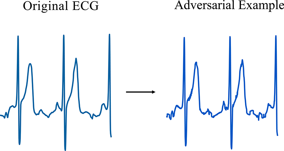
Traditional adversarial attack algorithms add a small imperceptible perturbation to lower the prediction accuracy of a machine learning model. However, attacking ECG deep learning classifiers with traditional methods creates examples that display square wave artifacts that are not physiologically plausible (Extended Data Fig. 1). By taking a weighted average of nearby time steps, we crafted smooth adversarial examples that cannot be distinguished from original ECG signals but will still fool the deep network to make a wrong prediction (See Methods).
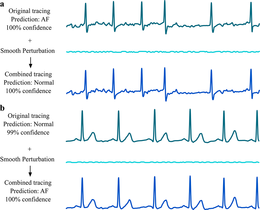
We generated adversarial examples on the test set. We transformed the test examples to make the network change the label of Normal, Other, and Noise to any other label. For AF, we altered the AF test examples so that the deep neural network classifies them as Normal. We can also alter Normal, AF, Other, and Noise to any given label. We show the results in Table 1. Misdiagnosis of AF as Normal may increase the risk of AF-related complications such as stroke and heart failure. We showcase the generation of adversarial examples in Fig. 1.
Table 1|. Success rate of targeted smooth attack method.
The original class is the class into which the network classifies the signal before the adversarial attack. The target class is the class into which the adversarial attack aimed to make the network classify the signal after adding. The success rate is calculated as the percentage of examples from the original class that were misclassified by the network to the target class after the adversarial attack.
| Target Class | |||||
|---|---|---|---|---|---|
| Normal | AF | Other | Noise | ||
| Original class | Normal | / | 57% | 55% | 13% |
| AF | 74% | / | 87% | 22% | |
| Other | 72% | 76% | / | 20% | |
| Noise | 79% | 64% | 57% | / | |
Fig. 1|. Demonstration of disruptive adversarial examples.
a, Example of an original ECG tracing that was correctly diagnosed by the network as atrial fibrillation (AF) with 100% confidence, but, after the addition of smooth perturbations, was diagnosed wrongly as normal sinus rhythm (Normal) with 100% confidence. b, Example of an original ECG tracing that was correctly diagnosed by the network as normal sinus rhythm with 100% confidence, but after the addition of smooth perturbations was diagnosed wrongly as AF. Perturbation and tracing voltages are plotted on the same scale.
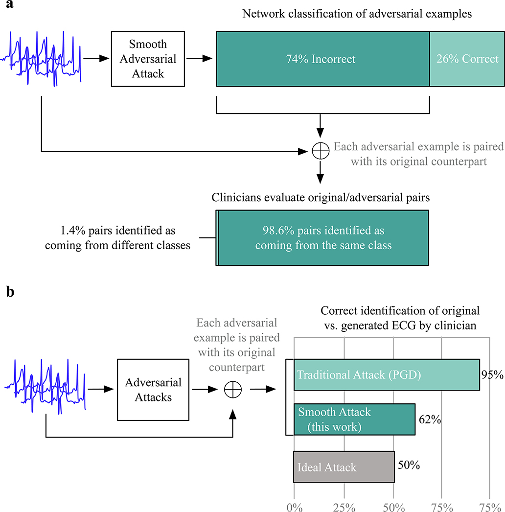
After adversarial attacks, 74% of the test ECGs originally classified correctly by the network are now assigned a different diagnosis, ultimately showing that deep ECG classifiers are vulnerable to adversarial examples. To assess how the generated signals would be classified by human experts, we invited one board certified medicine specialist and one cardiac electrophysiology specialist to diagnose whether signals generated by our methods and original ECGs come from the same class. Figure 2a shows that almost all of the modified signals were judged as belonging to the same class as the original signal. This shows that the deep network failed to correctly classify most of the newly generated examples, when a human would have assigned only 1.4% of them to a different class.
Fig. 2|. Accuracy of the network in classifying adversarial examples and clinician success rate in distinguishing authentic ECGs from adversarial examples.
a, Top, schematic showing that a smooth adversarial attack generated adversarial examples of ECG tracings that were misclassified in 74% of cases. Bottom, schematic showing that surveyed clinicians concluded that 246.5/250 pairs of adversarial examples and the original ECGs belonged to the same class. b, Schematic showing the success rate of ECG interpretation experts in distinguishing between 100 pairs of original ECGs and adversarial examples generated by the traditional attack method (PGD), the smooth attack method and the ideal attack method. The ideal attack method creates signals that clinicians cannot distinguish completely from the original signals.
We also invited the clinical specialists to distinguish ECG signals from the adversarial examples generated by our smooth method and the traditional attack method based on projected gradient descent (PGD)12,13. The question we asked is “Which one in the pair is the real ECG?” The calculated probability of correctly identifying ECGs is the number of correct answers they obtained for each pair over the number of pairs we showed them. The doctors were not shown adversarial examples beforehand.
Figure 2b shows that the adversarial examples generated by our method are significantly harder for clinicians to distinguish from the original ECG than the traditional attack method. On average, the clinicians were able to correctly identify the smoothed adversarial examples from their original counterpart 62% of the time. (The electrophysiology specialist was slightly more accurate at 65% versus 59%.) PGD examples are easier for clinicians to detect because of square wave discontinuity artifacts that are not physiologically plausible. These discontinuities also appear in PGD examples for images, but in images they get hidden by the resolution and color channels.
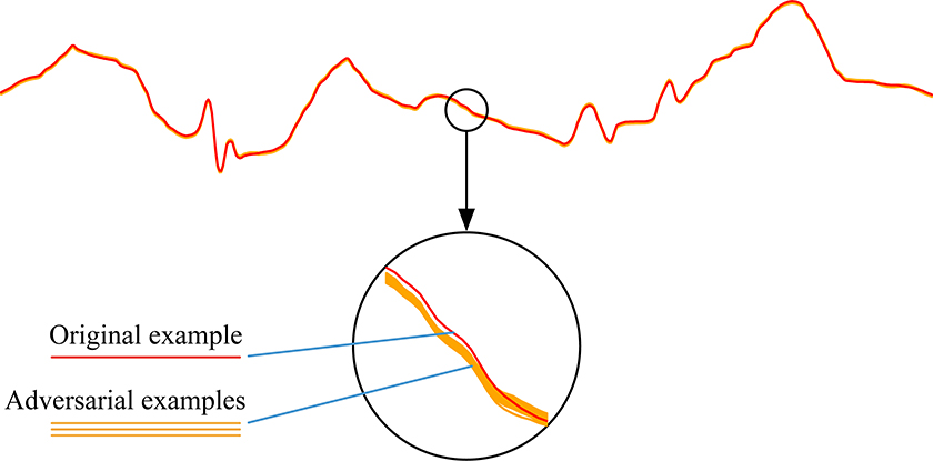
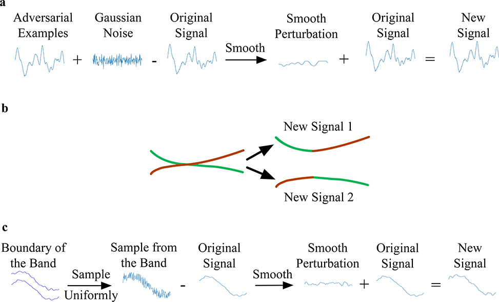
Here we provide a construction that shows that adversarial examples are not rare. In particular, we show that it is possible to create more examples that remain adversarial by adding a small amount of Gaussian noise to an original adversarial example and then smoothing the result. We repeat this process 1,000 times and find that the deep neural network still incorrectly classifies all 1,000 new, adversarial examples. Adding Gaussian noise could still produce adversarial examples on 87.6% of the test examples from which adversarial examples were generated. We plotted all of the newly crafted adversarial examples, which form a band around the original ECG signal, as shown in Fig. 3. The signals in the band may intersect. We chose pairs of intersecting signals and concatenated the left half of one signal with the right half of the other to create a new example. We found that signals created by concatenation are also adversarial examples. We also sampled random values in the band for each time step and then smoothed them to create new adversarial examples. These different perturbations on adversarial examples all led to new examples that remain mislabeled. This means that the adversarial examples should not be considered rare isolated cases, in that from a single adversarial example, many more can be created.
Fig. 3|. Perturbing a known adversarial example to generate multiple new ones.
Schematic showing that 1,000 different adversarial examples can be generated from the original ECG signal by adding small Gaussian noise and smoothing. The newly generated adversarial examples as well as the original ECG signal are plotted at the top. A portion of the original ECG signal and adversarial examples is enlarged in the circle below; the newly generated examples form a wide band around the original example.
The use of machine learning algorithms as a healthcare tool for clinical interpretation and prediction is seeing an unprecedented surge. A search in Pubmed for the phrases “electrocardiogram” AND (“machine learning” OR “artificial intelligence”) yields over 1200 publications. Specifically, deep learning has been utilized recently to create algorithms that predict the ejection fraction14, predict the susceptibility to QT prolongation in patients with normal QT intervals (https://www.alivecor.com/research/investigational-qt/artificial-intelligence-and-deep-neural-networks/) and identify patients with hyperkalemia15 -- all based on the ECG and demographics, without any additional clinical information. This promising ability of deep learning algorithms to reduce the cost or improve the performance of complex and laborious daily clinical challenges is creating significant incentive for rapid implementation and approval as practical clinical tools. Correspondingly, 23 machine learning algorithms, many that use deep learning, have been approved by the FDA for medical use in 2018 alone, a 283% increase from 2017 (https://medicalfuturist.com/fda-approvals-for-algorithms-in-medicine/). Products for arrhythmia classification with single-lead ECGs such as the Apple Watch, which sold over 20 million units in 2018 alone (https://ww.9to5mac.com/2019/02/27/apple-watch-sales-2018/) and the Alivecor Kardia, which uses deep learning and has recorded over 25 million ECGs (https://www.alivecor.com/press/press_release/alivecor-data-yield-reaches-25mm-ecgs/), are increasingly being adopted. Hence, it is imperative to understand the limitations and vulnerabilities of deep learning algorithms used to detect arrhythmia from ECGs.
In this work, we demonstrate the ability to add imperceptible perturbations to ECG tracings in order to create adversarial examples that fool a deep neural network classifier into assigning the examples to an incorrect rhythm class. Moreover, we showed that such examples are not rare.
These findings question the safety of using deep learning in analyzing ECGs at scale where millions of tests may be run every week by widespread consumer devices. To increase robustness to adversarial examples, it is crucial that classification methods for ECGs, especially those intended to operate without human supervision, generalize well to new examples. However generalization may be a significant challenge, because different environments and different devices can introduce unknown perturbations to the signal. Thus, ensuring safe generalization would require obtaining labeled data from each new environment and new device.
One way to protect against adversarial examples is adversarial training. Adversarial training works by generating adversarial examples repeatedly during model training based on the current model and adding them to the training batch used to improve the model12. However, such approaches can only protect against known adversarial examples, created with a given specific attack method, and are not guaranteed to protect against future attack methods. (See Methods for detailed discussions.) A more direct approach would be to certify deep neural networks for robustness with mathematical proofs16,17 as suggested for other safety-critical domains, such as the aviation industry18.
The possibility to construct even a single adversarial example may still enable malicious actors to inject small perturbations into RWD that are indistinguishable to the human eye. Indistinguishability matters to malicious actors to ensure they cannot be discovered by human auditors. The ability to create adversarial examples is an important issue, with future implications including the robustness to the environmental noise of medical devices that rely on ECG interpretation (for example, pacemakers, defibrillators)19, the skewing of data to alter insurance claims4 and the introduction of intentional bias into clinical trials. For example, imagine a large clinical trial intended to assess the effect of a treatment on reducing arrhythmias. Such a trial could use a pretrained neural network to identify how many arrhythmias occurred. Attacking this pretrained network could inject bias into the clinical trial by changing ECGs to reduce the number of documented arrhythmias. To prevent such possibilities, it is paramount that platforms for collection and analysis of RWD implement principles from ‘trusted computing’ to provide trusted data provenance guarantees that can certify that data has not been tampered with from device acquisition to any downstream analysis20. In this vein, closed systems without access to the raw ECG reduce malicious actor’s practical ability to attack systems. For devices where only the test signal can be modified, it is still possible to train a different network and generate adversarial examples using the blackbox attack from ref.12. For commercial devices such as the Apple Watch, malicious actors can potentially get access to many forward passes and construct examples using only the forward passes to solve the optimization problem used to construct smoothed adversarial examples21. If access to the full model is available, gradient-based attacks can be directly implemented.
One thing to note is that the lack of robustness observed is not inherent to the use of statistical methods to classify ECGs. Humans tend to be more robust to small perturbations because they use coarser visual features to classify ECGs, such as the R-R interval and the P-wave morphology. These features change less under small perturbations and generalize better to new domains. To automate the classification of more complex ECG tracings, it may be useful to incorporate hierarchical coarse pattern-dependent classification models along with deep learning to not only increase robustness to adversarial attacks but also to improve network accuracy. Additionally, regularizing deep networks to prefer coarser features can improve robustness. Tree-based learning algorithms using coarser features will also be more robust to attacks.
In conclusion, with this work, we do not intend to cast a shadow on the utility of deep learning for ECG analysis, which undoubtedly will be useful to handle the volumes of physiological signals available in the near future. This work should, instead, serve as an additional reminder that machine learning systems deployed in the wild should be designed with safety and reliability in mind22, with a particular focus on training data curation and provable guarantees on performance.
Methods
Description of the Traditional Attack Methods
Two traditional attack methods are the fast gradient sign method (FGSM)23 and PGD12,13. They are white-box attack methods based on the gradients of the loss used to train the model with respect to the input. Both FGSM and PGD can be used for targeted attacks and untargeted attacks. Targeted attacks force the network to output a specific incorrect label, while untargeted attacks force the network to make any wrong classification. Untargeted attacks usually minimize the probability of the true class; targeted attacks maximize the probability of the target class.
Denote our input entry x, true label y, classifier (network) f, and loss function L(f(x),y). We describe FGSM and PGD below:
-
Untargeted Attack
-
- FGSM: FGSM is a fast algorithm. For
an attack level ε, FGSM setsThe attack level is chosen to be sufficiently small so as to be undetectable.
-
- PGD: PGD is an improved version that uses multiple iterations of FGSM. Define Clipx,ε(x′) to project each x′ back to the infinity norm ball by clamping the maximum absolute difference value between x and x′ to ε. Beginning by setting , we have
(1) After T steps, we get our adversarial example .
-
-
Targeted Attack (target class t)
- - FGSM: For an attack level ε, FGSM sets
-
- PGD: Beginning by setting , we have
Unlike untargeted attacks, the gradient is subtracted. After T steps, we get our adversarial example .
In this Letter, we use targeted attacks to change AF to Normal and untargeted attacks on classes besides AF.
Our Smooth Attack Method
To smooth the signal, we use convolution. Convolution takes the weighted average of one position of the signal and its neighbors:
where a is the objective function and v is the weight or kernel function. In our experiment, the weights are determined by a Gaussian kernel. Mathematically, if we have a Gaussian kernel of size 2K + 1 and standard deviation σ, we have
We can easily see that when σ goes to infinity, the convolution with the Gaussian kernel becomes a simple average; when σ goes to zero, the convolution becomes the identity function. Instead of getting an adversarial perturbation and then convolving it with the Gaussian kernels, we could create adversarial examples by optimizing a smooth perturbation that fools the neural network. We introduce our method of training ‘smooth Adversarial Perturbations ‘(SAP). In our SAP method, we take the adversarial perturbation as the parameter θ and add it to the clean examples after convolving with a number of Gaussian kernels. We denote K(s,σ) to be a Gaussian kernel with size s and standard deviation σ. The resulting adversarial example can be written as a function of θ:
In our experiment, we let s be {5,7,11,15,19} and σ be {1.0, 3.0, 5.0, 7.0, 10.0}. Then we try to maximize the loss function with respect to θ to get the adversarial example in an untargeted attack. We still use PGD but this time on θ:
| (2) |
There are two major differences between updates Equation (2) and Equation (1). In Equation (2), we update θ not xadv and clip around zero not the input x. In practice, we initialize the adversarial perturbation θ to be the one obtained from PGD (ϵ = 10,α = 1,T = 20) on x and run another PGD (ϵ = 10,α = 1,T = 40) on θ.
For targeted attacks (target class t), the update is:
If we take the same combination of convolution on the adversarial examples generated in PGD to create smooth adversarial examples, 71% of the originally classified correctly test ECGs are assigned different labels, which is worse than our smooth attack method (74%). The idea of optimizing parameters of a smooth model could be expanded to other models, such as differential equation models of ECGs24 to find adversarial examples that more closely match human physiology.
Existence of Adversarial Examples
Our experiments are designed to show that adversarial examples are not rare. We only discuss untargeted attacks, but it is easy to extend our analysis to targeted attacks. Denote the original signal by x and adversarial example we generate by xadv.
First, we generate Gaussian noise and then add it to the adversarial examples. To make sure the new examples are still smooth, we smooth the perturbation by convolving with the same Gaussian kernels in our smooth attack method. We then clip the perturbation to make sure that it is still in the infinity norm ball. The newly generated example is
We repeat the process of generating new examples 1000 times. These newly generated examples are still adversarial examples. Some of them may intersect. For each intersected pair, we concatenate the left part of one example and the right part of the other to create new adversarial examples. Denote x1 and x2 to be a pair of adversarial examples that intersect. Suppose they intersect at time step t and the total length of the example is T. The new hybrid example x′ satisfies:
where [1:t] means from time step 1 to time step t. All the newly concatenated examples are still misclassified by the network.
The 1000 adversarial examples form a band. To emphasize that all the smooth signals in the band are still adversarial examples, we sample uniformly from the band to create new examples. Denote max[t] and min[t] to be the maximum value and minimum value of 1000 samples at time step t. To sample a smooth signal from the band, we first sample a uniform random variable for each time step t and then we smooth the perturbation. The example generated by uniform sampling and smoothing is
We repeat this procedure 1000 times. All of the newly generated examples still cause the network to make the wrong diagnosis. We visualize the three procedures to show the existence of adversarial examples in Extended Data Fig. 2.
Limitations of Adversarial Training
Adversarial training12 is a more effective method to build robust models than including adversarial examples in the training data. However, adversarial training does well only on small image datasets like MNIST25, not larger ones like CIFAR1026. For CIFAR10, even dynamically including adversarial examples while training the model will not lead to a robust model27. In addition, there is no formal guarantee that adversarial training implemented with PGD can converge to the saddle point of the infinity norm minimax formulation of adversarial training. For example, switching to a higher order optimizer may produce different adversarial examples not captured by PGD-based adversarial training.
Statistics and reproducibility
Figure 1a,b was generated for 50 AF signals and 124 normal sinus rhythms. Figure 3 was generated twice. Extended Data Fig. 1 was generated for 40 examples. We obtained similar results for the examples we generated.
Reporting Summary
Further information on research design is available in the Nature Research Reporting Summary linked to this article.
Data availability
The dataset can be accessed from https://physionet.org/challenge/2017/}{https://physionet.org/challenge/2017/
Code Availability
The code is available from https://github.com/XintianHan/ADV_ECG}{https://github.com/XintianHan/ADV\_ECG
Extended Data
Extended Data Fig. 1.
An adversarial example created by Projected Gradient Descent (PGD) method. This adversarial example contains square waves that are physiologically implausible.
Extended Data Fig. 2.
Demonstration of three procedures to show the existence of the adversarial examples. a, We add a small amount of Gaussian noise to the adversarial example and smooth it to create a new signal. b, For intersected signals, we concatenate the left half of one signal with the right half of the other to create a new one. c, We sample uniformly from the band and smooth to create a new signal.
Acknowledgements
X.H. and R.R. was supported in part by the NIH under award number R01HL148248. We thank W.L., S.M., M.G., A.L., A.M.P., H.S., M.S. and W.W..
Footnotes
Competing interests
The authors declare no competing interests.
Reference
- 1.Hannun AY, et al. Cardiologist-level arrhythmia detection and classification in ambulatory electrocardiograms using a deep neural network. Nature medicine 25, 65 (2019). [DOI] [PMC free article] [PubMed] [Google Scholar]
- 2.Szegedy C, et al. Intriguing properties of neural networks. in International Conference on Learning Representations (ICLR, 2014). [Google Scholar]
- 3.Biggio B et al. Evasion attacks against machine learning at test time. In Machine Learning and Knowledge Discovery in Databases Vol. 8190 (eds Blockeel H, Kersting K, Nijssen S & Železný F) 387–402 (Springer, 2013). [Google Scholar]
- 4.Finlayson SG, et al. Adversarial attacks on medical machine learning. Science 363, 1287–1289 (2019). [DOI] [PMC free article] [PubMed] [Google Scholar]
- 5.Paschali M, Conjeti S, Navarro F & Navab N Generalizability vs. robustness: investigating medical imaging networks using adversarial examples. in International Conference on Medical Image Computing and Computer-Assisted Intervention 493–501 (Springer, 2018). [Google Scholar]
- 6.Clifford GD, et al. AF Classification from a short single lead ECG recording: the PhysioNet/Computing in Cardiology Challenge 2017. in 2017 Computing in Cardiology (CinC) 1–4 (IEEE, 2017). [DOI] [PMC free article] [PubMed] [Google Scholar]
- 7.Kelly BB & Fuster V Promoting cardiovascular health in the developing world: a critical challenge to achieve global health, (National Academies Press, 2010). [PubMed] [Google Scholar]
- 8.Kennedy HL The evolution of ambulatory ECG monitoring. Progress in cardiovascular diseases 56, 127–132 (2013). [DOI] [PubMed] [Google Scholar]
- 9.Hong S, et al. ENCASE: An ENsemble ClASsifiEr for ECG classification using expert features and deep neural networks. in 2017 Computing in Cardiology (CinC) 1–4 (IEEE, 2017). [Google Scholar]
- 10.Chen H, Huang C, Huang Q & Zhang Q ECGadv: Generating Adversarial Electrocardiogram to Misguide Arrhythmia Classification System. arXiv preprint arXiv:1901.03808 (2019). [Google Scholar]
- 11.Goodfellow SD, et al. Towards understanding ecg rhythm classification using convolutional neural networks and attention mappings. in Machine Learning for Healthcare Conference 83–101 (2018). [Google Scholar]
- 12.Madry A, Makelov A, Schmidt L, Tsipras D & Vladu A Towards deep learning models resistant to adversarial attacks. in International Conference on Learning Representations (ICLR, 2018). [Google Scholar]
- 13.Kurakin A, Goodfellow I & Bengio S Adversarial machine learning at scale. in International Conference on Learning Representations, (ICLR, 2017). [Google Scholar]
- 14.Kwon J. m., et al. Development and validation of deep-learning algorithm for electrocardiography-based heart failure identification. Korean circulation journal 49, 629–639 (2019). [DOI] [PMC free article] [PubMed] [Google Scholar]
- 15.Galloway CD, et al. Development and Validation of a Deep-Learning Model to Screen for Hyperkalemia From the Electrocardiogram. JAMA cardiology 4, 428–436 (2019). [DOI] [PMC free article] [PubMed] [Google Scholar]
- 16.Singh G, Gehr T, Mirman M, Püschel M & Vechev M Fast and effective robustness certification. in Advances in Neural Information Processing Systems 10802–10813 (2018). [Google Scholar]
- 17.Cohen J, Rosenfeld E and Kolter Z Certified Adversarial Robustness via Randomized Smoothing. In International Conference on Machine Learning 1310–1320 (ICML, 2019). [Google Scholar]
- 18.Julian KD, Kochenderfer MJ & Owen MP Deep neural network compression for aircraft collision avoidance systems. Journal of Guidance, Control, and Dynamics 42, 598–608 (2018). [Google Scholar]
- 19.Nguyen MT, Van Nguyen B & Kim K Deep Feature Learning for Sudden Cardiac Arrest Detection in Automated External Defibrillators. Scientific reports 8, 17196 (2018). [DOI] [PMC free article] [PubMed] [Google Scholar]
- 20.Lyle J & Martin A Trusted computing and provenance: better together. (Usenix, 2010). [Google Scholar]
- 21.Uesato J, O’Donoghue B, Kohli P and Oord A Adversarial Risk and the Dangers of Evaluating Against Weak Attacks. In International Conference on Machine Learning 5025–5034 (ICML, 2018). [Google Scholar]
- 22.Saria S & Subbaswamy A Tutorial: Safe and reliable machine learning. arXiv preprint arXiv:1904.07204 (2019). [Google Scholar]
Reference
- 23.Goodfellow IJ, Shlens J & Szegedy C Explaining and harnessing adversarial examples. in International Conference on Learning Representations (ICLR, 2015). [Google Scholar]
- 24.McSharry PE, Clifford GD, Tarassenko L & Smith LA A dynamical model for generating synthetic electrocardiogram signals. IEEE transactions on biomedical engineering 50, 289–294 (2003). [DOI] [PubMed] [Google Scholar]
- 25.LeCun Y, Bottou L, Bengio Y & Haffner P Gradient-based learning applied to document recognition. Proc. IEEE 86, 2278–2324 (1998). [Google Scholar]
- 26.Krizhevsky A & Hinton G Learning multiple layers of features from tiny images. (Citeseer, 2009). [Google Scholar]
- 27.Schmidt L, Santurkar S, Tsipras D, Talwar K & Madry A Adversarially robust generalization requires more data. in Advances in Neural Information Processing Systems 5014–5026 (NIPS, 2018). [Google Scholar]
Associated Data
This section collects any data citations, data availability statements, or supplementary materials included in this article.
Data Availability Statement
The dataset can be accessed from https://physionet.org/challenge/2017/}{https://physionet.org/challenge/2017/


