The Thermospheric Column O/N₂ Ratio

Abstract

More than 2 decades ago, D. J. Strickland and colleagues proposed use of the O/N₂ column number density ratio as a new geophysical quantity to interpret thermospheric processes recorded in far ultraviolet (FUV) images of the Earth. This concept has enabled multiple advances in understanding the global behavior of Earth’s thermosphere. Nevertheless, confusion remains about the conceptual meaning of the column density ratio, and in the application of this integral quantity. This is so even though it is now a key thermospheric measurement made by current and planned far ultraviolet remote sensing missions in pursuit of new understanding of thermospheric processes and variability. The intent here is to review the historical context of the O/N₂ column density ratio, clarify its physical meaning, and resolve misunderstandings evident in the literature. Simple examples elucidate its original derivation for extracting column O/N₂ ratios from measurements of the OI 135.6 nm/N₂ Lyman-Birge-Hopfield (LBH) emission based on an algorithmic synthesis of model precomputations. These are organized in the form of a table lookup of column density ratio as a function of observed radiance ratios. To accommodate generalized solar-geophysical and viewing conditions, the table required to specify the number of needed parameters becomes large. Proposed as an alternative is a simplified, first principles approach to obtaining the column density ratio from the emission ratio. This new methodology is now being applied successfully to FUV measurements made from onboard the Ionospheric CONnection satellite and will be applied retrospectively to the Global Ultraviolet Imager data.

1. Geophysical Concept

1.1. Origins

Images of the far ultraviolet (FUV) dayglow observed in the direction of the Earth’s disk have been made for more than 40 years, for example by the Apollo 16 Lunar Camera (Carruthers & Page, 1976a, 1976b), the Dynamics Explorer (Frank and Craven, 1988) and the POLAR missions (Germany et al., 1994; Frank et al., 1995; Torr et al., 1995). Often these observations were used to provide context for in situ measurements without requirement for quantitative assessment. Despite the application of forward models to assess magnitudes and morphologies of the imaged emission rates (e.g., Drob et al., 1998; Germany et al., 1994; Meier et al., 1995) and empirical models to assess variability (Immel et al., 2000), the extraction of quantitative atmospheric composition information from the data proved challenging because the FUV disk images depict column emission rates (CER) without revealing the altitudes where the signal originates. In contrast, observations of the ultraviolet emission from Earth’s limb do contain quantitative information (e.g., Meier & Anderson, 1983; Meier & Picone, 1994; Meier et al., 2015) because their altitude variations above the horizon allow extraction of composition profiles.

Strickland et al. (1995) overcame the disk problem, for the first time, by demonstrating a functional relationship between the ratios of observed far ultraviolet airglow emission intensities and the ratios of the column densities of O and N₂. The latter quantity is designated herein as ΣO/N₂ to distinguish the ratio of column densities from the volume density ratio, O/N₂. Strickland et al. found minimal ambiguity in the relationship when the vertical column densities are calculated above an altitude, z₁₇, corresponding to an N₂ column (from infinity down to z₁₇) of 10¹⁷ cm⁻² (= N_N2 in Equation 1; N_O is the O column density above z₁₇). Thus, ΣO/N₂ is defined as:

$$\Sigma \frac{\text{O}}{{\text{N}}_2}\equiv \frac{{\int }_{z_{17}}^{\infty }{n}_{\text{O}}\text{d}z}{{\int }_{z_{17}}^{\infty }{n}_{{\text{N}}_2}\text{d}z}=\frac{{\int }_0^{N_{\text{O}}}\text{d}{N}_{\text{O}}^{\prime }}{{\int }_0^{N_{{\text{N}}_{\text{2}}}}\text{d}{N}_{{\text{N}}_2}^{\prime }}=\frac{N_{\text{O}}}{{10}^{17}{\text{\hspace{0.17em}cm}}^{-2}}.$$ (1)

At N_N2 = 10¹⁷ cm⁻², Strickland et al. found little dependence of the relationship between ΣO/N₂ and the 135.6 nm/LBH emission ratio on the details of the model atmosphere, although they did find a dependence on solar zenith angle and viewing angle from nadir (Evans et al., 1995). The main point of their discovery is that the column density ratio can be found from the ratio of disk radiances without knowing how O and N₂ are distributed throughout the atmosphere.

Further, they were able to quantify the solar extreme ultraviolet (EUV) energy flux required to produce the observed airglow by using the absolute magnitude of either the O or the N₂ CERs. Strickland et al. designated this solar variable as Q_euv the integral over wavelength of the model solar spectral irradiance from 1 to 45 nm, in units of W m⁻², a quantity directly comparable to independent measurements of solar EUV spectral irradiance (e.g., Woods et al., 2008). This allows for determination of the internal consistency of the FUV airglow observations and extracted geophysical quantities.

Subsequent studies arising from the pioneering work of Strickland et al. (1995) leave no doubt about the geophysical importance of ΣO/N₂ and the value of its close relationship to O and N₂ FUV emission rates. Embodied in Equation 1 is the prescription for comparison of observed ΣO/N₂ to atmospheric model predictions: simply integrate the model N₂ density vertically downward until the altitude (z₁₇) is found where the column density is 10¹⁷ cm⁻². Next, the O column density is computed above that altitude and divided by 10¹⁷ to obtain the model ΣO/N₂ for comparison with observations. This definition of altitude is only needed for comparison with models. It does not violate the Strickland et al. finding that the ΣO/N₂ retrieved from observed OI 135.6/N₂ LBH has little dependence on the altitudinal distribution of composition.

For an atmosphere in pure diffusive equilibrium, ΣO/N₂ is independent of temperature. A simple example of this independence is an isothermal atmosphere: temperature cancels in the ratio of O to N₂ scale heights. The independence is also true for the Bates-Walker (Walker, 1965) and Jacchia (1977) diffusive equilibrium models. But in realistic atmospheres, column density ratio and temperature can be related. For example, high latitude joule heating causes upwelling that results in increased molecular concentrations relative to atomic oxygen. This lower ΣO/N₂, hotter air is redistributed globally by equatorward winds, especially at night, that can result in dramatic changes in the column density ratio (Meier et al., 2005). I have even noticed high latitude decreases in GUVI observations of ΣO/N₂ for very weak geomagnetic activity increases in Ap from 2 to 4. As well, Crowley et al. (2008) have related 7- and 9-days oscillations in the solar wind to modulation of ΣO/N₂ by vertical winds at high latitudes and by inference, thermal expansion at low latitudes.

In summary, it is now established that observed “two-color” disk images of FUV dayglow emissions (i.e., measured at oxygen and nitrogen wavelengths) are readily convertible into a geophysically meaningful quantity, ΣO/N₂ which, in turn, can be analyzed with simulations by atmospheric models. Research incorporating and comparing observed and modeled ΣO/N₂ has established the dramatic responsivity of this ratio to thermospheric dynamical processes that change the abundance of O relative to N₂ (e.g., Crowley et al., 2008; Meier et al., 2005; Zhang et al., 2004). A connection between ΣO/N₂ and both F-region peak electron density and total electron content is also apparent (e.g., Lean, Meier, et al., 2011; Strickland et al., 2001), surmised to be the result of ionospheric F-region photochemistry that relates the volume densities of electrons to O/N₂ in photochemical equilibrium.

So far, this paper has categorically referred to the N₂ emission rate in the denominator of the Strickland et al. algorithm as “LBH.” Specifically, it means emission from the a¹Π_g electronic state of the molecule to the X ¹Σ_g⁺ ground state. Details of the LBH spectrum used by Strickland et al. (1995) and in this paper are taken from Conway (1982). Conway’s spectral synthesis includes bands ranging from 127.3 to 360 nm. So, it is important to define what is meant by “LBH.” The definition depends on the type of measurement; so a unique Strickland et al. algorithm must be derived for each instrument. For the ICON FUV instrument, the LBH channel covers the wavelength range, 152–162 nm, with peak responsivity at 158 nm (Mende et al., 2017). Convolution of the instrument responsivity with the LBH emission spectrum results in a measurement of 6.8% of the total band emission. FUV remote sensing missions should always report the fraction of the total LBH band that is observed.

1.2. Conceptual Confusion

Much of the current confusion about the thermospheric column O/N₂ ratio and its geophysical interpretation concerns the reference altitude, z₁₇, for which the N₂ column reaches 10¹⁷ cm⁻². Some researchers have attempted to assign geophysical significance to this altitude, by postulating that it is a fundamental variable (Yu et al., 2020; Zhang & Paxton, 2011, 2012). Strickland et al. (2012) objected to this interpretation, asserting that “the proper and necessary way to understand O concentration changes from satellite observations of OI 135.6 nm and N₂ LBH dayglow from the Earth’s disk is not in terms of altitude but in terms of column densities, including total column density.”

The present study aims to resolve this argument by demonstrating with explicit examples in Sections 2 and 3, that ΣO/N₂ must follow the Strickland et al. interpretation in terms of thermospheric column density (or equivalently optical depth). Strickland et al. found that the relationship between ΣO/N₂ and the 135.6 nm/LBH ratio becomes less accurate for column densities less than or greater than N_N2 = 10¹⁷ cm⁻². The way to understand this is to recognize that the emission rates are sensitive to the atmospheric column where the solar EUV radiation is deposited. At column base less than N_N2 = 10¹⁷ cm⁻², the lower accuracy is likely a consequence of not including in the algorithm, the production of airglow by solar EUV photons that have passed through to greater column depths. Similarly, for a column density base in excess of N_N2 = 10¹⁷ cm⁻², there is little or no airglow production, so the numerator and denominator of Equation 1 needlessly include large non-contributing values that reduce the accuracy of the relationship between the column density ratio and the emission rate ratio. An N₂ column density base of 10¹⁷ cm⁻² defines a region that contains most of the photon production and therefore results in the optimal algorithmic relationship for sunlight incident on a terrestrial atmosphere.

1.3. Other Complexities

As aforementioned, the simple relationship between column density ratio and emission rate ratio does depend on the solar zenith angle and the viewing angle from nadir. Consequently, when viewing the disk away from nadir, the azimuth angle relative to the solar azimuth angle also becomes an essential parameter—viewing toward the sun leads to a different result than viewing away from the sun. Figure 1 illustrates the geometric concepts. The azimuth of the instrument line of sight (LOS) is of minimal importance near the subsolar location but becomes critically important for observations approaching twilight.

Figure 1.

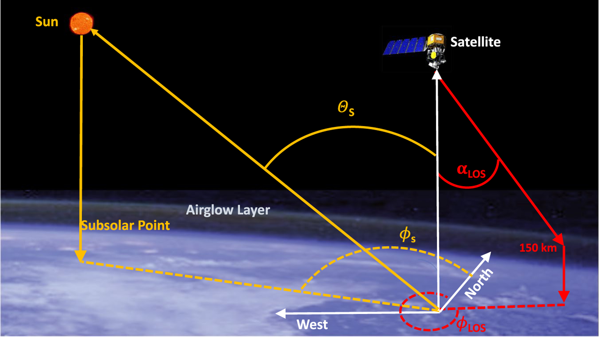
Illustration of typical observing geometry. α_LOS is the view angle of the instrument from local nadir, ϕ_LOS is the azimuth from north of the line of sight (LOS) projection onto a plane at 150 km altitude perpendicular to the local vertical. θ_S is the solar zenith angle and ϕ_S is the solar azimuth relative to north. All azimuth angles are measured counterclockwise relative to north.

Later investigations have revealed additional effects that influence the dependence of the column density ratio on the emission rate ratio. For example, variations in the spectral distribution of the solar EUV irradiance can affect the relationship, both over a solar cycle and during solar flares. This is a consequence of wavelength dependence of the atmospheric absorption cross sections that effectively move the energy deposition to different column depths (Strickland et al., 2007). And, as this paper describes, there is actually a slight dependence on atmospheric composition (less than ~2%) of the relationship of the 135.6/LBH ratio to ΣO/N₂ when evaluated over a larger range of atmospheres than used by Strickland et al. (1995). As explained later, this is undoubtedly due to the inclusion of physical effects traceable to O₂ or to instrumental configuration.

In the most general case, accurate retrieval of ΣO/N₂ from measurements of the 135.6/LBH ratio therefore requires knowledge of 1) the solar zenith angle, 2) the view angle from nadir and 3) its azimuth relative to the sun’s azimuth (Figure 1), 4) the solar EUV spectral irradiance, and 5) atmospheric concentrations. The solar spectrum and the minimal atmospheric effects are readily accommodated in the algorithm by including a priori information from empirical models that are dependent on solar activity. For nadir viewing, there is no azimuthal effect; even up to 20° from nadir the error from using a fixed azimuth is less than a few per cent. Nonetheless, an accurate algorithm suitable for any atmospheric observation must include all five parameters. Alternatively, this paper proposes a generalized approach for the extraction of ΣO/N₂ from radiance ratios.

Section 2 discusses the basic principles that relate the observed airglow ratios to thermosphere ΣO/N₂ and Section 3 establishes the irrelevance of the reference altitude. Section 4 assesses effects of neglecting the various parameters in a table lookup algorithm. Section 5 describes the new approach for retrieving column O/N₂ from OI 135.6 nm to N₂ LBH emissions, a methodology that abolishes the need for a five-parameter table.

2. Why is the Airglow Intensity Ratio Proportional to the Column O/N₂ Ratio?

The production of FUV emission is initiated by solar EUV radiation incident on and absorbed by the atmosphere. Following absorption by atmosphere gases, photons with wavelengths shorter than about 45 nm have enough energy to photoionize O and N₂, releasing photoelectrons with energy sufficient to excite the FUV dayglow (45 nm corresponds to 15.4 eV photoionization energy of N₂ plus 12 eV photoelectron energy). Such photoelectrons can then inelastically collide with O and N₂, exciting them to the ⁵S and a¹Π_g electronic states, respectively. The relaxation of excited species to their ground states produces OI 135.6 nm and N₂ LBH photons. Using altitude for the benefit of visualization, the profiles of the volume emission rates of these species peak between 150 and 200 km, depending on solar activity, atmospheric conditions and solar zenith angle. The topside profiles (at altitudes above the emission peak) mostly follow the O and N₂ scale heights with some modification due to the photoelectron flux profile. The bottom sides of the emitting layers (at altitudes below the emission peak) decrease rapidly with decreasing altitude due to extinction of the solar EUV radiation. Meier (1991), and Strickland et al. (1999) provide examples of such profiles.

O and N₂ column emission rates are line-of-sight integrals of the volume emission rate modified by extinction and scattering along the line-of-sight. Further examination of volume emission rates in the above publications shows that the base of the emitting column is in the vicinity of, or slightly larger than, N_N2 = 10¹⁷ cm⁻² (although there is a smaller level of FUV radiation coming from deeper in the atmosphere due to soft X-ray production of photoelectrons and from multiple scattering of 135.6 nm photons). Thus, the atmosphere’s emission of both 135.6 nm and LBH radiation mostly originates in a column whose base ranges in model atmospheres from about 135–140 km and whose meaningful top is between 200 and 300 km altitude. It is important to recognize that the column emission rates are related to the column densities and are not a measure of the number density at 135–140 km.

A semi-quantitative derivation of the radiance ratio relationship to column density ratio follows. The column emission rate is given by the integration over altitude of the volume emission rate, which is the product of the photoelectron g-factor (excitation rate per sec per atom) and the number density, n at altitude z. Assumed for simplicity is a nadir observing direction from a space-based platform above the atmosphere. Minor multiple scattering effects of the 135.6 nm radiation field are ignored (typically <10% in the region of peak photon production), as is pure absorption by O₂ that takes place lower in the atmosphere. (The vertical optical depth for O₂ extinction reaches unity at 135.6 nm around 110 km, so it plays little role in affecting the vertical column emission rate which samples much higher altitudes. On the other hand, O₂ extinction for limb viewing takes place at much higher altitudes due to the long slant path through the atmosphere; typically, the atmosphere becomes opaque below tangent altitudes of about 130 km. This allows retrieval of the O₂ concentration from limb scanning data.) The g-factor at each altitude (excitation s⁻¹) is defined as the integration over energy, E of the (isotropic where collisions dominate) photoelectron flux, Φ(E) (electron cm⁻² s⁻¹ ev⁻¹) times the electron impact excitation cross section, σ(E): g = ∫ Φ(E) σ(E) dE. For LBH bands, the excitation cross section is for the vibrational bands being observed. With these approximations, the ratio of the 135.6/LBH column emission rates (in Rayleighs) is

$$\frac{4\pi I_{1356}}{4\pi I_{\text{LBH}}}=\frac{{\int }_{zl}^{\infty }{g}_{1356}(z)n_O(z)\text{d}z/{10}^6}{{\int }_{zl}^{\infty }{g}_{\text{LBH}}(z)n_{N_2}(z)\text{d}z/{10}^6}.$$ (2)

Converting more precisely to column density as the independent variable, the emission ratio becomes:

$$\frac{4\pi I_{1356}}{4\pi I_{\text{LBH}}}=\frac{{\int }_0^{N_{\text{O}}^l}{g}_{1356}(N_{\text{O}})\text{d}{N}_{\text{O}}}{{\int }_0^{N_{{\text{N}}_2}^l}{g}_{\text{LBH}}(N_{{\text{N}}_2})\text{d}{N}_{{\text{N}}_2}}\cong \frac{g_{1356}^{\text{eff}}}{g_{\text{LBH}}^{\text{eff}}}\cdot \frac{N_{\text{O}}^l}{N_{{\text{N}}_2}^l}.$$ (3)

The lower limit on the integrals, z_l in Equation 2, is the altitude that includes the FUV emitting column (i.e., z₁₇). The right-hand side of Equation 3 assumes that an effective column density exists such that the relationship between intensity ratio and column density ratio is unique. This assumption is not strictly true in a real atmosphere where there is curvature of the slope of the radiance ratio-column density ratio relationship due to the effects mentioned above that this derivation ignores. Nevertheless, it is now clear from Equation 3 why Strickland et al. (1995) were able to obtain a definitive relationship between the radiance and column density ratios.

The proportionality between the column emission rate ratio and the column density ratio can be represented generally by defining S as the slope of the relationship:

$$\frac{4\pi I_{1356}}{4\pi I_{\text{LBH}}}=S\left(\Sigma \text{O}/{\text{N}}_2,X\right)\cdot \Sigma \text{O}/{\text{N}}_2,$$ (4)

where X is a vector representing the remaining five parameters. Traditionally the functionality of S is the synthesized numerically from forward modeling and organized into a lookup table.

3. Irrelevance of Reference Altitude

What is the significance of the column density base? In their search to quantify the association of disk emission rates and thermospheric column densities, Strickland et al. (1995) established that a nearly unique relationship exists only when the base of the column integrals is properly defined. As noted above, this turned out to be the location where N_N2 = 10¹⁷ cm⁻² in the terrestrial atmosphere. To determine this, they used the AURIC model (Strickland et al., 1999) to compute disk emission rates for a large number of model atmospheres, demonstrating with thousands of computations that the ratio of OI 135.6 nm to N₂ LBH emission rates is ordered very well by the then-new concept of ΣO/N₂.

Strickland et al. (2012, 1995) already pointed out that the correct way to interpret the relationship of Equation 4 is through the column density as the independent variable. The fundamental point is that Equations 1 and 3 demonstrate the irrelevance of the number density distribution along the emitting path.

Simple examples readily prove the mathematical relationship between the radiance ratio and the column density ratio independent of the distribution of the number densities. The examples are executed by applying Equation 2 to a cloud of mixed O and N₂ gas. In this idealized situation there is no reference to altitude, per se. The cloud is assumed to be uniform in the plane perpendicular to the solar direction and of sufficiently large column depth to absorb all solar EUV radiation. A variety of gas mixtures is used, including uniform number densities of O and N₂, linear variation of O relative to N₂, Heaviside (square wave) layers of O and N₂, and exponential variations. As will be seen, these examples corroborate the derivation of Equation 4 from Equation 2.

The first group of examples assumes g-factors that are a simple exponential function of total column density, N, as shown in Equation 5 and in the dashed lines of Figure 2. N is chosen because that is the independent parameter used by Strickland et al. (1997) in their parameterized

$$g_i(N)=g_i(0)e^{-N/N_e},$$ (5)

model of g-factors. This typifies excitation rates associated with direct photon excitation into excited states of the species, i, rather than by photoelectron excitation; as such it is easily integrable. In this case, the g-factor at the sunward edge of the cloud is the integration over energy of the solar irradiance times the excitation cross section. Although not necessary for the purpose of illustration, the exponential g-factors are chosen so that their magnitudes and 1/e extinction values (N_e) are comparable to the photoelectron g-factors (solid lines).

Figure 2.

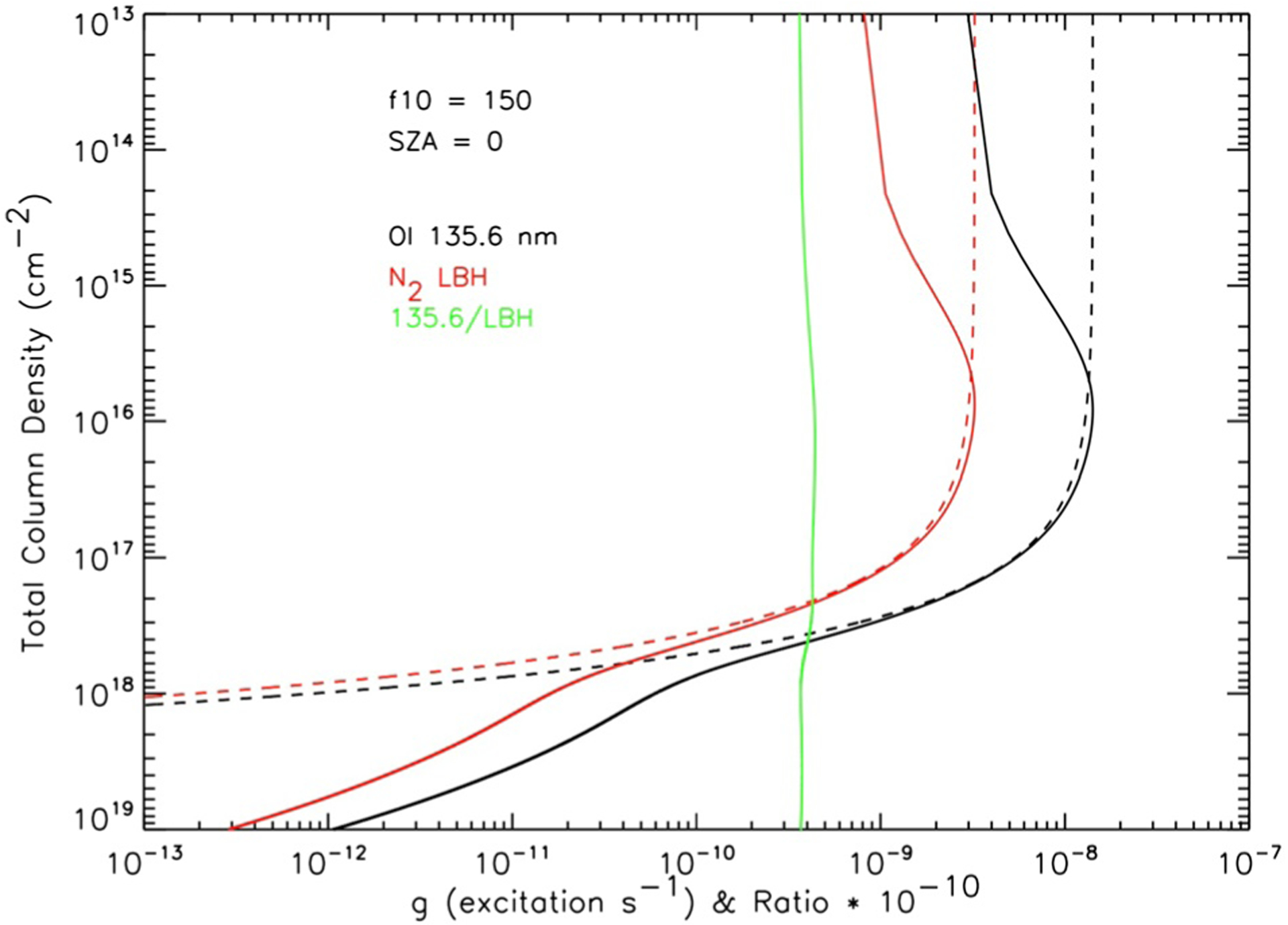
Photoelectron (solid) and exponential (dashed) g-factors are plotted against overhead total column density from the Sun. OI 135.6 nm excitation is in black and N₂ LBH band is in red. The ratio of the photoelectron g-factors is in green. The solar 10 cm flux is 150 SFU. LBH, Lyman-Birge-Hopfield.

A uniform mixture of O and N₂ is defined as constant volume densities throughout the cloud. The O and N₂ column densities thus increase linearly with depth into the cloud, and the exponential g-factor extinction causes the volume excitation rate (g·n) to decrease. Substitution of Equation 5 and constant n values into Equation 2 leads to,

$$\frac{4\pi {\text{I}}_{1356}}{4\pi {\text{I}}_{\text{LBH}}}=\frac{g_{\text{O}}(0)}{g_{{\text{N}}_2}(0)}\cdot \Sigma \text{O}/{\text{N}}_2.$$ (6)

Thus, in this straightforward example, the intensity ratio depends linearly on the column density ratio and the column density ratio is independent of distance into the cloud. Analytic and numerical computations of ratios using the remaining three volume density distributions (linear, Heaviside, and exponential) all fall on the same straight line described by Equation 6.

It is straightforward to repeat the same exercise using the photoelectron g-factors plotted in Figure 2. For simplicity, these were computed using the analytic representation proposed by Strickland et al. (1997) rather than a numerical computation of the photoelectron flux. All four density distributions produced a linear relationship, although the ratio of g-factors differs from the exponential g-factor.

4. Table Lookup Algorithm

The Strickland et al. (1995) proposal for retrieving ΣO/N₂ from 4πI_135.6 / 4πI_LBH entailed precomputation of tables of the two quantities versus solar zenith angle (Evans et al., 1995), primarily for viewing in the nadir from satellite altitude. The column density ratio is quickly and easily found from a measurement of the two radiances through two-dimensional interpolation or direct table lookup with very fine gridding of the tabular values of radiance ratio and solar zenith angle. As emphasized in Section 1, for more general viewing conditions, the solar spectrum, the model atmosphere, and the viewing geometry all play a role in and increase the dimensionality of the table.

To illustrate the table lookup algorithm and to estimate the level of error expected if the table fails to include parameters beyond the solar zenith angle, a forward model is used to construct a table for selected conditions. The forward model incorporates the NRLSSI-EUV solar EUV spectral irradiance, updated from Lean, Woods, et al. (2011) using more recent SEE data (Solar EUV Experiment; Woods et al., 2018); the NRLMSIS00 (Picone et al., 2002) model atmosphere; and an abbreviated version of the AURIC algorithm (Meier et al., 2015; Strickland et al., 1999) to compute the photoelectron excitation rates. In all test cases herein, the algorithm database is restricted to a fixed model atmosphere for F10.7 = 150 SFU (a Solar Flux Unit = 10⁻²² watt per square meter-hertz = 10,000 Jansky), day of year = 70, latitude = 0°, longitude = 0°, and local solar time = 8 H. The azimuth relative to the sun is set at 90° (i.e., ϕ_LOS = 0 and ϕ_S = 90° in Figure 1). The hypothetical observation is made toward the earth disk from 525 km, well above emission altitudes. Because most observations of the OI 135.6 nm emission rate are contaminated by the underlying LBH band near that wavelength, the examples herein assume the same for realism. Using the ICON FUV instrument as an example, the total signal in the 1,365.6 nm channel contains 12.2% of the total LBH band emission rate. For the pure LBH channel, a single band at 158 nm is used in this restricted example that includes 6.8% of the total LBH emission. For simplicity, the O₂ pure absorption cross section is evaluated only at these two test wavelengths. (Note that the actual ICON algorithm includes the full LBH vibrational band structure in each of the FUV channels along with the correct description of O₂ extinction.) Thus, this test algorithm is parameterized only by vertical column density, solar spectral irradiance variability, and solar zenith angle. This allows for error estimates using “observed” radiances computed with the forward model using known solar, atmospheric (i.e., number and column densities), and viewing conditions.

Figure 3 gives an example of the basic table lookup process. In this case, the noiseless “observations” for illustrating the algorithm use a solar EUV spectral irradiance and model atmosphere defined by F10 = 70 SFU, appropriate for current (2020) conditions. The solar zenith angle of the observer in this test is 55°. Numerical values of the “observed” column emission rates are included in the figure; their ratio is 5.59. The black curves are from the algorithm tables using F10 = 70 SFU; tabular values are indicated by the small + symbols. The algorithm first interpolates across solar zenith angles to produce the red curve in the figure at 55°. Tracing the straight red line vertically upward from 5.59 on the abscissa to the red curve leads to 1.085 for the retrieved column density ratio on the ordinate. The retrieved column density ratio is in excellent agreement with the “true” value from the forward model, 1.088.

Figure 3.

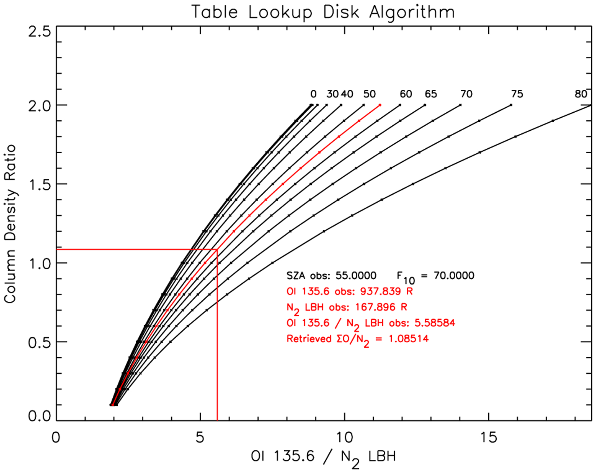
Illustration of the table lookup algorithm. Precomputed database of column density in the algorithm is plotted as a function of the intensity ratio for solar zenith angles labeled at the top of each black curve. The tabular grid intervals are marked as the small black points on the curves and the solid lines are interpolations. For an “observed” ratio of about 5.59 at 55° solar zenith angle, the retrieved column density ratio is 1.085, as indicated by the vertical and horizontal straight red lines connecting at the interpolated red curve.

As pointed out earlier, ideally, families of curves like those shown in Figure 3 are required for each level of solar activity, model atmosphere, angle from local nadir, and azimuth from the sun. Error, often significant, is possible if these parameters are not included in the algorithm. Selected error estimates are provided next in order to probe the performance of the table lookup algorithm when it does not accommodate all parameters. Specifically, radiance ratios for the “true” model atmosphere are computed using varying solar EUV irradiances, model atmospheres, and viewing conditions. The fixed-condition algorithm then retrieves column density ratios for comparison with the “true” column density ratios and their errors are determined for selected conditions. These are “estimates” because they are meant to typify the level of error, but not to constitute a rigorous error analysis for the full range of solar-geophysical and viewing configurations. For simplicity, the first two examples are restricted to nadir viewing.

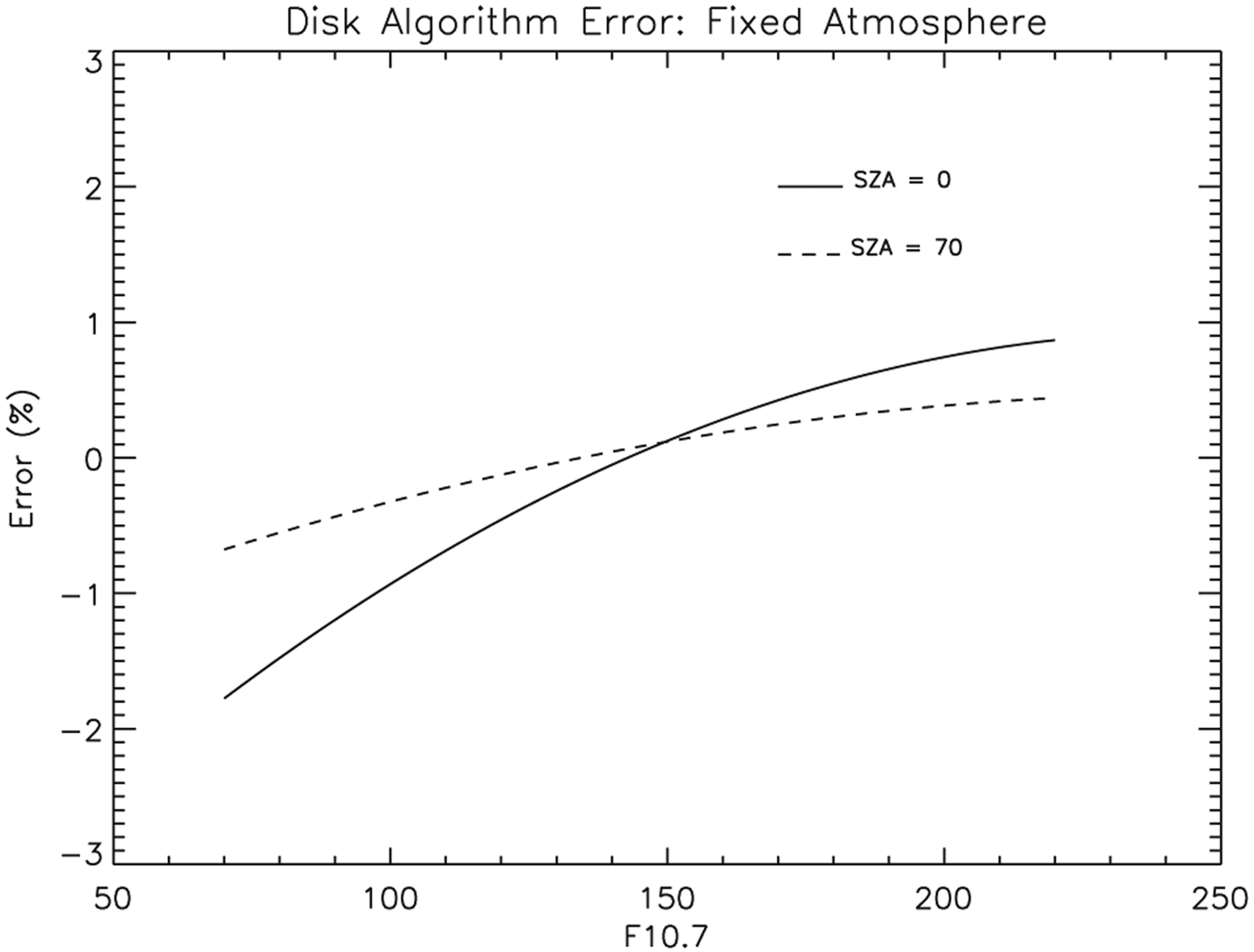
The first example assesses the error in the retrieved ΣO/N₂ caused by the fixed solar spectral irradiance of the algorithm. In order to isolate the solar activity effect from the atmospheric changes, NRLMSIS00 is fixed at F10 = 150 SFU in the forward model. The algorithm returns for varying F10 are plotted in Figure 4 for 0° and 70° solar zenith angle. Errors of up to 10% are obtained with a fixed irradiance algorithm. Strickland et al. (2007) discuss in more detail the effect of the solar spectrum on the column density retrieval.

Figure 4.

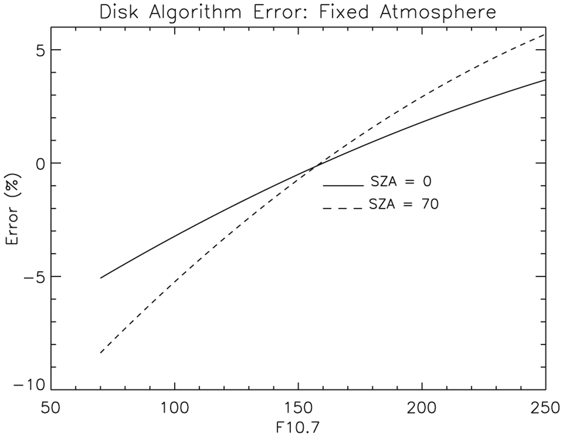
Estimated algorithmic error from using a fixed solar EUV spectrum is plotted against solar EUV spectral irradiance characterized by the 10.7 cm radio flux. For this example, the NRLSSI-EUV solar spectral irradiance model changes with F10.7 in the forward model for emission ratio computations, but the NRLMSIS00 model atmosphere is fixed at F10 = 150 SFU. See text for geographic and local time information. EUV, extreme ultraviolet.

The second example uses “observed” (nadir) emission rates computed with a constant solar spectral irradiance (NRLSSI-EUV with F10 = 150 SFU) in order to isolate the effect of a varying atmosphere. Figure 5 displays the resulting error of the fixed sun algorithm. Unlike the simple examples in Section 3, a small dependence on composition is present for a realistic atmosphere, undoubtedly due to ignoring factors such as O₂ extinction, contamination of the OI 135.6 nm emission by LBH bands and the minor contribution of photoelectron impact on O₂ resulting dissociative excitation of O (⁵S).

Figure 5.

Estimated error from using a fixed model atmosphere in the algorithm is plotted against solar activity. The NRLMSIS00 model in the emission ratio computations varies with F10, but the NRLSSI-EUV solar spectral irradiance model is fixed at F10 = 150 SFU. See text for geographic location and local time information. EUV, extreme ultraviolet.

The last example assesses the error in retrieved ΣO/N₂ for off nadir viewing. In this situation, it is essential to accommodate the variation of the solar illumination along the line of sight (as implemented by Meier et al., 2015 in the GUVI algorithm). The error is not symmetric toward and away from the sun because the exponential extinction of sunlight is greater for viewing away from the sun. Recall that the algorithm database was computed for a fixed azimuth of −90° relative to the solar azimuth (ϕ_LOS = 0 and ϕ_S = 90° in Figure 1). With the sun and the observer located in the equatorial plane, the azimuth is toward the north in the algorithm. Noiseless “observations” for evaluating the fixed-azimuth disk algorithm were computed for six angles relative to nadir: α_LOS = 0°, 10°, 20°, 40°, 60°, and 70°. The azimuths for each nadir angle, ϕ_LOS range from 0° to 360°.

Figure 6 shows the errors in retrieved ΣO/N₂ at solar zenith angle θ_S = 60° as a function of azimuth, ϕ_LOS. Each curve is for the different angles, α_LOS from nadir. As expected, there is minimal error for small angles from nadir. Even at 60° from nadir, the maximum error reaches only about ±5%. But there is a substantial increase for larger nadir angles as the geographic difference between the solar illumination along the LOS toward and away from the sun becomes large. For a smaller θ_S = 30°, the errors between the forward model and the fixed azimuth algorithm are less than ±1% up to 20° from nadir, are less than ±2% up to 40° from nadir and reach ±10% at 70° from nadir. At 75° solar zenith angle the error is even larger for viewing away from nadir. At 40° from nadir, the error is about ±5% and at 60° and 70° from nadir, the error reaches 10% and 40%, respectively.

Figure 6.

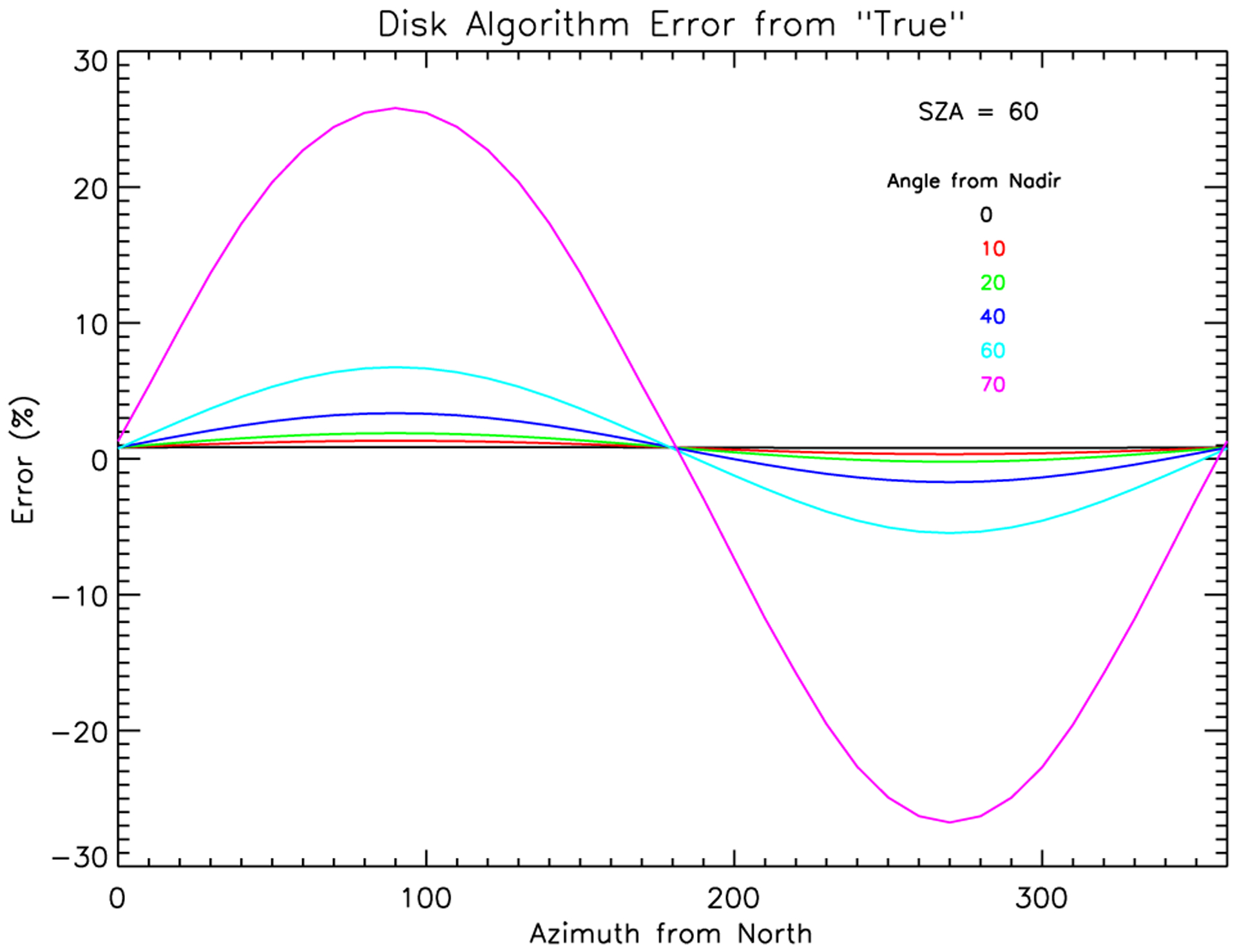
Estimated errors expected from using a fixed azimuth in the algorithm. The model atmosphere and the solar EUV radiance are both fixed in the forward model used to compute the emission ratios, with F10 = 150 SFU and solar zenith angle of 60°. The observer and the sun are on the equator, so the solar azimuth from North is 90°. Each curve is for a different angle from nadir. EUV, extreme ultraviolet.

While the error plots in Figures 4–6 are indicative of the effects of three different parameters on the value of ΣO/N₂ retrieved from FUV emission ratios, the full range of parameter space is larger than that explored here. Nonetheless, these examples demonstrate the importance of parameterizing the solar-geophysical conditions and the viewing angles in table lookup algorithms for other than a few limited situations.

5. Alternative Disk Algorithm

Launched into a 600 km altitude, 27° inclination orbit on October 10, 2019, the ICON FUV instrument images Earth’s limb from about 500 km tangent altitude downward onto the disk to an angle of about 58° from nadir. At this closest approach to nadir, the azimuth angle of the line of sight relative to the solar azimuth can vary by more than 50° around the orbit. Based on the analysis of Section 3, a traditional algorithm that successfully extracts ΣO/N₂ from ICON disk data requires a table lookup with five parameters in order to meet the mission requirement of 8% accuracy. This could lead to numerical challenges, especially if interpolation of the table is required.

To avoid such issues, a new and more concise technique for extracting ΣO/N₂ from the disk 135.6 nm to LBH band ratio was proposed. It is new because all previous algorithmic approaches have employed lookup tables. Although the table lookup method uses first principles models to populate the table, the new methodology employs the first principles model directly. The process consists of the following steps:

1. Compute the 135.6 nm and LBH band emissions with a forward model that incorporates the viewing geometry, the best prediction of the solar EUV irradiance and model atmosphere, and a representation of the instrument characteristics

2. Compute the predicted vertical column density ratio, ΣO/N₂ at a standard location, such as the pierce point, where the line of sight passes through the 150 km level (Figure 1)

3. Scale the predicted ΣO/N₂ up and down by a specified increment (e.g., multiply the O concentration by 0.5 and 1.5) and recompute the 135.6 nm/LBH radiance ratios for the higher and lower column density ratios to create three emission rate ratios

4. Fit the three column density ratios versus radiance ratios with a simple polynomial or interpolate to find the value of ΣO/N₂ for the observed radiance ratio

Step 1) of the procedure accounts for four of the parameters that determine ΣO/N₂. It includes physical effects left out in the simplified examples of Sections 2 and 3, such as multiple scattering of 135.6 nm photons, production of O (⁵S) from dissociative excitation of O₂ by energetic photoelectrons, O₂ extinction and an instrument model. For the present example, the instrument model is a simplified version of the actual ICON FUV forward mode described by Stephan et al. (2018). The ICON model is highly customized for the mission and lacks the flexibility for tests such as these. The simplified model uses responsivities at 135.6 nm and at 158 nm only (instead of the detailed character of emissions within the spectral band of an actual instrument). The responsivities were selected to match the effective values of the ICON FUV instrument, 0.59 and 0.20 counts/R, respectively for the two wavelengths. Step 4) is analogous to the red curve in Figure 3. This method, of course, assumes that the scaling in Step 3) encompasses the observed emission rate ratios. If it does not, the range of values can be expanded beyond 50% to avoid extrapolation errors. Comparisons against the table lookup algorithm (under restricted viewing conditions) and against limb retrievals (e.g., Meier et al., 2015) of the column O/N₂ yield excellent results; estimated uncertainties in the retrieved values are a small fraction of a percent and could be improved with higher precision coding.

One the many possible tests of the new algorithmic approach consists of generating synthetic data for known solar-geophysical conditions. Disk retrievals of ΣO/N₂ can then be carried out for comparison with radiance ratios from the known atmosphere and satellite observing conditions. A convenient test case is a typical ICON orbit and disk viewing case—58° from nadir. Synthetic data are generated by applying counting noise to a forward model computation of disk radiances. Random counting noise is generated using the responsivities of the two FUV detectors to convert computed radiances into counts, apply Poisson noise and convert back into Rayleighs. The model atmosphere and solar spectral irradiance are for solar medium conditions with F10 = 150 SFU.

The upper left panel in Figure 7 shows synthetic data versus time for the short wavelength channel (SW), which includes both OI 135.6 and 12.2% of the total N₂ LBH band, as explained earlier in Section 4 for the ICON FUV instrument. The long wavelength channel (LW) includes 6.8% of the entire LBH band emission. The upper right panel in Figure 7 shows their ratios. The lower left panel shows the coordinates for the so-called pierce point, where the line of sight of the instrument passes through a surface at 150 km altitude level above the reference ellipsoid (Figure 1)— the ICON standard for geolocating disk retrievals. The lower right panel contains the data points obtained from the new algorithm, as well as the “truth” that is, the NRLMSIS00 model. The mean of the difference between the retrievals and the “truth” is virtually zero and the standard deviation of the data points is about 8%.

Figure 7.

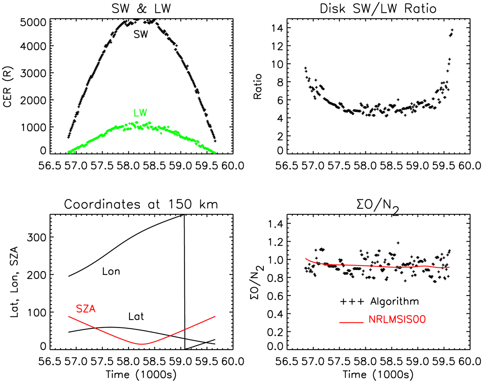
Simulation of the new disk ΣO/N₂ retrieval algorithm for a typical ICON orbit. In the upper left panel, synthetic data for viewing at 58° from nadir are plotted versus time into a simulated ICON orbit. SW is the short wavelength (135.6 nm + 12.2% of the LBH band) channel and LW is the long wavelength (6.8% of the LBH band) channel. The upper right is the ratio of SW to LW emissions. The lower left panel gives the coordinates for each point at the location where the line of sight passes through 150 km altitude. The black points in the lower right panel are the values retrieved with the algorithm and the red line is the “truth.” The solar activity level is F10 = 150 SFU. ICON, Ionospheric CONnection; LBH, Lyman-Birge-Hopfield; LW, long wavelength.

6. Discussion and Conclusions

The motivation for the tutorial on the physical foundation of the column density ratio concept in Sections 1–3 is to preclude future misinterpretation of the thermospheric information available from the ratios, as exemplified by the argument between Zhang and Paxton (2012) and Strickland et al. (2012). Equation 3 and Section 2 of this paper demonstrate that no information about the altitude distribution of O and N₂ is available from ΣO/N₂ derived from remote sensing. Contrary to the claim by Zhang and Paxton (2011) that the altitude base of the column, z₁₇ is a fundamental parameter, their approach actually requires the introduction of a priori information about altitude in the form of an atmospheric model. While it is true that an observation of the column density ratio can constrain a model, the correctness of the altitude variations within the model can only be known with additional information.

More recently, Yu et al. (2020) used an empirical argument based on GUVI limb observations to assert that the altitude of the column base can be obtained from the column density ratio. GUVI limb data are scans of the Earth limb from near 500 km down to 110 km tangent altitudes and are readily inverted to obtain altitude profiles of O, N₂, and O₂ (Meier et al., 2015). The column density ratio may then be computed through vertical integration of the number densities (Equation 1) and taking the ratio. But this method of retrieving ΣO/N₂ is obviously not a direct disk measurement. Rather, it is only the knowledge of the altitude distribution inherent in the limb scans that allows the base of the column to be quantified. While there may be some correlation between ΣO/N₂ and z₁₇, there is no guarantee that a disk measurement alone can specify the base of the column without the introduction of additional altitude information. Indeed, the correlation in their Figure 6a shows tens of km spread in actual z₁₇ versus their empirical model—much larger than the ~5 km uncertainty obtained from a prediction by the NRLMSIS00 model alone. (Note that the NRLMSIS 2.0 is more accurate at solar minimum; Emmert et al., 2020).

The advent of the ICON (Immel et al., 2018) and GOLD missions (Eastes et al., 2020) has exposed the limitations of the standard disk algorithm for the retrieval of the O/N₂ column density ratio from the OI 135.6 nm/N₂ LBH band ratio. The table lookup algorithm required to accommodate all viewing conditions is cumbersome in its most generalized form. A new concise algorithm is described that overcomes a numerically simple but potentially challenging five parameter table lookup. A distinct advantage of the new method is that the same forward model used in limb retrievals is applied to disk data—no precomputed synthesis is required. This avoids the dilemma, as yet unresolved in the GUVI data, namely the precomputed table lookup disk algorithm produces different column density ratios than does the limb inversion algorithm (Meier et al., 2015).

The new algorithm has been implemented for ICON FUV disk data processing at the Science Data Center, U. California, Berkeley. Again, the algorithm used for ICON is more sophisticated and customized than that used in Section 5. It includes all physical effects contributing to the observed emissions as well as the detailed characteristics of the FUV instrument.

As amply demonstrated by Strickland and colleagues, by others over the years, and by this work, the O/N₂ column density ratio has now become a standard geophysical parameter that offers much in diagnosing the state of the thermosphere, particularly on global scales. Reflecting this, thermospheric models should now routinely offer output fields of ΣO/N₂ for ready analysis of observations.

Key Points:

• A tutorial is presented describing the thermospheric column O/N2 ratio retrieved from the ratio of OI 135.6 nm/N2 LBH emissions

• A new concise method of retrieving column ratios from emission ratios avoids the need for a five-parameter table lookup

• The new methodology is currently in use with the ICON far ultraviolet data and will be applied to existing GUVI data

References

- Carruthers GR, & Page T (1976a). Apollo 16 far ultraviolet imagery of the polar auroras, tropical airglow belts, and general airglow. Journal of Geophysical Research, 81, 483. 10.1029/ja081i004p00483 [DOI] [Google Scholar]
- Carruthers GR, & Page T (1976b). Apollo 16 Far ultraviolet spectra of the terrestrial airglow. Journal of Geophysical Research, 81, 1683. 10.1029/ja081i010p01683 [DOI] [Google Scholar]
- Conway RR (1982). Self-absorption of the N2Lyman-Birge-Hopfield bands in the far ultraviolet dayglow. Journal of Geophysical Research, 87, 859. 10.1029/ja087ia02p00859 [DOI] [Google Scholar]
- Crowley G, Reynolds A, Thayer JP, Lei J, Paxton LJ, Christensen AB, et al. (2008). Periodic modulations in thermospheric composition by solar wind high speed streams. Geophysical Research Letters, 35, L21106. 10.1029/2008GL035745 [DOI] [Google Scholar]
- Drob DP, Meier R, Picone JM, Strickland DJ, Cox RJ, & Nicholas AC (1998). Atomic oxygen in the thermosphere during the July 13, 1982 solar proton event deduced from far ultraviolet images. Journal of Geophysical Research, 104, 4267 [Google Scholar]
- Eastes RW, McClintock WE, Burns AG, Anderson DN, Andersson L, Aryal S, et al. (2020). Initial observations by the GOLD mission. Journal of Geophysical Research: Space Physics, 125, e2020JA027823. 10.1029/2020JA027823 [DOI] [Google Scholar]
- Emmert JT, Drob DP, Picone JM, Siskind DE, Jones M, Mlynczak MG, et al. (2020). NRLMSIS 2.0: A whole-atmosphere empirical model of temperature and neutral species densities. Journal Geophysical Research, e2020EA001321. 10.1029/2020EA001321 [DOI] [Google Scholar]
- Evans JS, Strickland DJ, Huffman RE, & Eastes RW (1995). Satellite remote sensing of thermospheric O/N2 and solar EUV, 2. Data analysis. Journal of Geophysical Research, 100, 12217–12226. 10.1029/95ja00573 [DOI] [Google Scholar]
- Frank LA, & Craven JD (1988). Imaging results from dynamics explorer I. Reviews of Geophysics, 2(6), 249–283. 10.1029/rg026i002p00249 [DOI] [Google Scholar]
- Frank LA, Sigwarth JB, Craven JD, Cravens JP, Dolan JS, Dvorsky MR, et al. (1995). The visible imaging system (VIS) for the polar spacecraft. Space Science Reviews, 71, 297–328. 10.1007/bf00751334 [DOI] [Google Scholar]
- Germany GA, Torr DG, Richards PG, Torr MR, & John S (1994). Determination of ionospheric conductivities from FUV auroral emissions. Journal of Geophysical Research, 99, 23297–23305. 10.1029/94ja02038 [DOI] [Google Scholar]
- Immel TJ, Craven JD, & Nicholas AC (2000). An empirical model of the OI FUV dayglow from DE-1 images. Journal of Atmospheric and Solar-Terrestrial Physics, 62, 47–64. 10.1016/s1364-6826(99)00082-6 [DOI] [Google Scholar]
- Immel TJ, England SL, Mende SB, et al. (2018). The ionospheric connection explorer mission: Mission goals and design. Space Science Reviews, 214, 13. 10.1007/s11214-017-0449-2 [DOI] [PMC free article] [PubMed] [Google Scholar]
- Jacchia LG (1977). Thermospheric temperature, density and composition: New models. Smithsonian Astrophysical Observatory Special Report; (Vol. 375). [Google Scholar]
- Lean JL, Meier RR, Picone JM, & Emmert JT (2011). Ionospheric total electron content: Global and hemispheric climatology. Journal of Geophysical Research, 116, A10318. 10.1029/2011JA016567 [DOI] [Google Scholar]
- Lean JL, Woods TN, Eparvier FG, Meier RR, Strickland DJ, Correira JT, & Evans JS (2011). Solar extreme ultraviolet irradiance: Present, past, and future. Journal of Geophysical Research, 116, A01102. 10.1029/2010JA015901 [DOI] [Google Scholar]
- Meier RR (1991). Ultraviolet spectroscopy and remote sensing of the upper atmosphere, Space Science Review, 58, 1–186. [Google Scholar]
- Meier RR, & Anderson DE (1983). Determination of atmospheric composition and temperature from the UV airglow. Planetary and Space Science, 31, 967. 10.1016/0032-0633(83)90088-0 [DOI] [Google Scholar]
- Meier RR, Cox R, Strickland DJ, Craven JD, & Frank LA (1995). Interpretation of dynamics explorer far UV images of the quiet time thermosphere. Journal of Geophysical Research, 100(A4), 5777. 10.1029/94JA02679 [DOI] [Google Scholar]
- Meier R, Crowley G, Strickland DJ, Christensen AB, Paxton LJ, Morrison D, & Hackert CL (2005). First look at the 20 November 2003 superstorm with TIMED/GUVI: Comparisons with a thermospheric global circulation model. Journal of Geophysical Research, 110, A09S41. 10.1029/2004JA010990 [DOI] [Google Scholar]
- Meier RR, & Picone JM (1994). Retrieval of absolute thermospheric concentrations from the far UV dayglow: An application of discrete inverse theory. Journal of Geophysical Research, 99(A4), 6307–6320. 10.1029/93JA02775 [DOI] [Google Scholar]
- Meier RR, Picone JM, Drob D, Bishop J, Emmert JT, Lean JL, et al. (2015) Remote sensing of earth’s limb by TIMED/GUVI: Retrieval of thermospheric composition and temperature. Earth and Space Science, 2. 10.1002/2014EA000035 [DOI] [Google Scholar]
- Mende SB, Frey HU, Rider K, Chou C, Harris SE, Siegmund OHW, et al. (2017). The far ultra-violet imager on the ICON mission. Space Science Reviews, 212(1), 655–696. 10.1007/s11214-017-0386-0 [DOI] [PMC free article] [PubMed] [Google Scholar]
- Picone JM, Hedin AE, Drob DP, & Aikin AC (2002). NRLMSISE-00 empirical model of the atmosphere: Statistical comparisons and scientific issues. Journal of Geophysical Research, 107(A12), 15. 10.1029/2002JA009430 [DOI] [Google Scholar]
- Stephan AW, Meier RR, England SL, Mende SB, Frey HU, & Immel TJ (2018). Daytime O/N2 retrieval algorithm for the ionospheric connection explorer (ICON). Space Science Reviews, 214, 42. 10.1007/s11214-018-0477-6 [DOI] [PMC free article] [PubMed] [Google Scholar]
- Strickland DJ, Bishop J, Evans JS, Majeed T, Shen PM, Cox RJ, et al. (1999). Atmospheric ultraviolet radiance integrated code (AURIC): Theory, software architecture, inputs, and selected results. Journal of Quantitative Spectroscopy and Radiative Transfer, 62, 689–742. 10.1016/S0022-4073(98)00098-3 [DOI] [Google Scholar]
- Strickland DJ, Craven JD, Daniell RE (2001). Six days of thermospheric-ionospheric weather over the northern Hemisphere in late September 1981. Journal Geophysical Research. 106, 30291–30306. 10.1029/2001JA001113 [DOI] [Google Scholar]
- Strickland DJ, Evans JS, & Correira J (2012). Comment on “Long-term variation in the thermosphere: TIMED/GUVI observations” by Zhang Y and Paxton LJ. Journal of Geophysical Research, 117, A07302. 10.1029/2011JA017350 [DOI] [Google Scholar]
- Strickland DJ, Evans JS, & Paxton LJ (1995). Satellite remote sensing of thermospheric O/N2 and solar EUV, 1, Theory. Journal of Geophysical Research, 100(12), 217. 10.1029/95ja00574 [DOI] [Google Scholar]
- Strickland DJ, Lean JL, Daniell RE, Knight HK, Woo WK, Meier RR, et al. (2007). Constraining and validating the Oct/Nov 2003 X-class EUV flare enhancements with observations of FUV dayglow and E-region electron densities. Journal of Geophysical Research, 112, A06313. 10.1029/2006JA012074 [DOI] [Google Scholar]
- Strickland DJ, Majeed T, Evans JS, Meier RR, & Picone JM (1997). Analytical representation of g-factors for rapid, accurate calculations of excitation rates in the dayside thermosphere. Journal of Geophysical Research, 102, 14485. 10.1029/97ja00943 [DOI] [Google Scholar]
- Torr MR, Torr DG, Zukic M, Johnson RB, Ajello J, Banks P, et al. (1995). A far ultraviolet imager for the international solar-terrestrial physics mission. Space Science Reviews, 71, 329–383. 10.1007/bf00751335 [DOI] [Google Scholar]
- Walker JCG (1965). Analytic representation of upper atmosphere densities based on Jacchia’s static diffusion models. Journal of the Atmospheric Sciences, 22, 462. 10.1175/1520-0469(1965)022<0462:arouad>2.0.co;2 [DOI] [Google Scholar]
- Woods TN, Chamberlin PC, Peterson WK, Meier RR, Richards PG, Strickland DJ, et al. (2008). XUV Photometer System (XPS): Improved solar irradiance algorithm using CHIANTI spectral models. Solar Physics, 250, 235–267. 10.1007/s11207-008-9196-6 [DOI] [Google Scholar]
- Woods TN, Eparvier FG, Harder J, et al. (2018). Decoupling solar variability and instrument trends using the multiple same-irradiance-level (MuSIL) analysis technique. Solar Physics, 293, 76. 10.1007/s11207-018-1294-5 [DOI] [PMC free article] [PubMed] [Google Scholar]
- Yu T, Ren Z, Yu Y, Yue X, Zhou X, & Wan W (2020). Comparison of reference heights of O/N2 and ΣO/N2 based on GUVI dayside limb measurement. Space Weather, 18, e2019SW002391. 10.1029/2019sw002391 [DOI] [Google Scholar]
- Zhang Y, & Paxton LJ (2011). Long-term variation in the thermosphere: TIMED/GUVI observations. Journal of Geophysical Research, 116, A00H02. 10.1029/2010JA016337 [DOI] [Google Scholar]
- Zhang Y, & Paxton LJ (2012). Reply to comment by Strickland DJ et al. on “Long-term variation in the thermosphere: TIMED/GUVI observations”. Journal of Geophysical Research, 117, A07304. 10.1029/2012JA017594 [DOI] [Google Scholar]
- Zhang Y, Paxton LJ, Morrison D, Wolven B, Kil H, Meng C-I, et al. (2004). O/N2 changes during 1–4 October 2002 storms: IMAGE SI-13 and TIMED/GUVI observations. Journal of Geophysical Research, 109, A10308. 10.1029/2004JA010441 [DOI] [Google Scholar]