

Abstract
The Global Modeling and Assimilation Office (GMAO) has recently released a new version of the Goddard Earth Observing System (GEOS) Sub-seasonal to Seasonal prediction (S2S) system, GEOS-S2S-2, that represents a substantial improvement in performance and infrastructure over the previous system. The system is described here in detail, and results are presented from forecasts, climate equillibrium simulations and data assimilation experiments.
The climate or equillibrium state of the atmosphere and ocean showed a substantial reduction in bias relative to GEOS-S2S-1. The GEOS-S2S-2 coupled reanalysis also showed substantial improvements, attributed to the assimilation of along-track Absolute Dynamic Topography. The forecast skill on subseasonal scales showed a much-improved prediction of the Madden-Julian Oscillation in GEOS-S2S-2, and on a seasonal scale the tropical Pacific forecasts show substantial improvement in the east and comparable skill to GEOS-S2S-1 in the central Pacific. GEOS-S2S-2 anomaly correlations of both land surface temperature and precipitation were comparable to GEOS-S2S-1, and showed substantially reduced root mean square error of surface temperature.
The remaining issues described here are being addressed in the development of GEOS-S2S Version 3, and with that system GMAO will continue its tradition of maintaining a state of the art seasonal prediction system for use in evaluating the impact on seasonal and decadal forecasts of assimilating newly available satellite observations, as well as to evaluate additional sources of predictability in the earth system through the expanded coupling of the earth system model and assimilation components.
1. Introduction
NASA’s Global Modeling and Assimilation Office (GMAO) develops and maintains the modular, configurable Global Earth Observing System (GEOS) modeling and data assimilation system. This flexible system is used for diverse applications, with an overarching goal of supporting NASA’s mission of Earth Observation. The applications include high-resolution atmospheric model simulations, the Modern-Era Retrospective analysis for Research and Applications, Version 2 (MERRA-2, Gelaro et al. [2017]), and sub-seasonal to seasonal (S2S) prediction. This study presents an overview of the structure and performance of the recently released Version 2 of the GEOS-S2S system, which includes a coupled Atmosphere-Ocean General Circulation Model (AOGCM), an ocean data assimilation system (ODAS), and a methodology for weakly coupled Atmosphere-Ocean Coupled Data Assimilation (AODAS).
Version 1 of the GEOS-S2S system ([Borovikov et al., 2017]), referred to as GEOS-S2S-1, has a long history of being successfully employed in seasonal prediction efforts and contributing to multi-system ensemble projects. For example, it was a participating model in the North American Multi-model Ensemble (NMME: [Kirtman et al., 2014]) since that project’s inception in 2011. GEOS-S2S forecasts are also routinely included in various other national and international multi-model ensembles including the multi-model forecast products at the International Research Institute for Climate and Society (IRI) of Columbia University; GMAO’s involvement in such projects enables rigorous evaluations of the system’s forecast skill and model biases and allows the quantification of GEOS-S2S system performance relative to that of other state-of-the art systems. The suite of GEOS-S2S-1 forecasts was expanded for Version 2, to include near-real-time weekly initialized forecasts at the subseasonal timescale, thereby facilitating GMAO’s participation in NOAAs experimental subseasonal multi-model ensemble project [Pegion et al., 2019].
Version 2 of the GEOS-S2S system (GEOS-S2S-2) is the first step in an aggressive development pathway for the GEOS system that will lead to a fully coupled ocean-atmosphere reanalysis designed to highlight the use of NASA’s space-based observations, emphasizing their impacts on subseasonal to seasonal prediction. This step builds on many changes to the GEOS model system and the analyses that have occurred since GEOS-S2S-1 was released in 2007. One important aspect in the timing of this upgrade was the termination of the original MERRA reanalysis on Feb. 29, 2016, and its replacement with MERRA-2.
GEOS-S2S-2 represents an important step by the GMAO towards a seamless prediction and data assimilation capability for the Earth System, encompassing prediction from weather to decadal time scales and horizontal resolutions ranging from 3 to 100 km. A key element has been the synchronization of GMAO development efforts for the version of the Atmospheric General Circulation Model (AGCM) included in the GEOS-S2S-2 system and the version currently in use for weather prediction. As such, prediction on seasonal and sub-seasonal time scales in GEOS-S2S-2 naturally benefited from the developments to improve atmospheric initial conditions for weather prediction and the assimilation of satellite observations (as embodied in MERRA-2 and the GMAO’s related near-real-time atmospheric analyses). GEOS-S2S-2 also benefited from model developments that addressed short term climate variability linked to coupling with the land surface, the stratosphere, and the ocean. Those developments are combined with major new infrastructure and capabilities in GEOS-S2S-2 that include the implementation of a Local Ensemble Transform Kalman Filter (LETKF, Penny et al [2013]) ocean analysis facilitating the assimilation of satellite altimetry data, an upgrade from the MOM4 to the MOM5 ocean model [Griffies et al., 2005; Griffies, 2012], the implementation of the Goddard Chemistry Aerosol Radiation and Transport (GOCART, Chin et al [2002]; Colarco et al [2010]) interactive aerosol model allowing experimental predictions of aerosol loadings, and the implementation of a two-moment cloud microphysics scheme [Barahona et al., 2014] which allows the inclusion of the aerosol indirect effect on clouds.
This paper provides a detailed description of GEOS-S2S-2, emphasizing the improvements over GEOS-S2S-1, and assesses the performance of climate, forecasts and data assimilation. Section 2 presents a description of the model and data assimilation system as well as the experiments performed here to evaluate the system. Sections 3, 4 and 5 provide, respectively, the evaluations of the simulated climate, of the data assimilation that underlies the forecast initialization, and of the forecasts themselves. A summary is provided in section 6.
2. Description of the Coupled Model, Data Assimilation System and Forecast Initialization
The GEOS AOGCM and the GEOS Atmosphere-ocean Data Assimilation System (AODAS) are designed to simulate the earth system on a wide range (synoptic to decadal) of time scales. The main components of the GEOS AOGCM are the GEOS atmospheric general circulation model [Molod et al., 2015; Rienecker et al., 2008], the catchment land surface model [Koster et al., 2000], the Goddard Chemistry Aerosol Radiation and Transport (GOCART) aerosol model [Chin et al, 2002; Colarco et al, 2010] the Modular Ocean Model-5 (MOM5) ocean general circulation model [Griffies et al., 2005; Griffies, 2012] and the Community Ice CodE-4 (CICE4) sea ice model [Hunke and Lipscomb, 2008]. The atmospheric data assimilation component is the pre-existing “Forward Processing for Instrument Teams” near-real-time assimilation (FPIT, FPIT [2016]), and the ocean data assimilation follows the Local Ensemble Transform Kalman Filter (LETKF) [Penny et al, 2013]. All components are coupled together using the Earth System Modeling Framework (ESMF, [Hill et al., 2004]) and the MAPL interface layer [Suarez et al., 2007]. Various operational centers are developing Coupled AODAS systems [Dee et al., 2014; Brassington et al., 2015], in which different components (e.g., atmosphere and ocean) of the earth system are analyzed separately [Laloyaux et al., 2016; Lea et al., 2015] or simultaneously [Sluka et al., 2016; Wada and Kunii, 2017]. The GEOS-S2S Coupled AODAS relies on an pre-computed near-real-time atmospheric analysis, and performs an analysis of the ocean state. Each of the components of the GEOS S2S Version 2 system will be described here in varying amounts of detail. More emphasis will be given to the ocean data assimilation and forecast procedures since the atmospheric data assimilation is already well documented (e.g. Gelaro et al. [2017]).
2.1. Coupled Atmosphere-Ocean General Circulation Model
2.1.1. Atmospheric, Land and Aerosol Models
The version of the GEOS AGCM that is used as part of the GEOS Seasonal to Subseasonal (S2S) prediction system Version 2 simulates large-scale transport and dynamics with an adaptation of the flux-form semi-Lagrangian (FFSL) finite-volume (FV) dynamics of Lin [2004], adapted for a cubed sphere horizontal discretization [Putman and Lin, 2007]. A comprehensive description of baseline versions of the physical parameterizations, which include convection, cloud macro- and micro-physics, longwave and shortwave radiation, turbulence, and gravity wave drag, is found in Rienecker et al. [2008], and the updates to a recent version of the AGCM are found in Molod et al. [2015].
Convection is parameterized using the Relaxed Arakawa-Schubert scheme [Moorthi and Suarez, 1992], prognostic cloud cover and cloud water and ice are determined by the two moment cloud microphysics parameterization of Barahona et al. [2014], and the probability distribution function (PDF) for total water that governs the cloud macrophysics is described by Molod [2012]. Longwave radiative processes are described by Chou and Suarez [1994], and shortwave radiative transfer is from Chou [1990, 1992]. The turbulence parameterization is based on the Lock scheme [Lock et al., 2000] combined with the Richardson-number based algorithm of Louis and Geleyn [1982]. The Monin-Obukhov surface layer parameterization is described by Helfand and Schubert [1995], and ocean surface roughness is determined by a blend of the algorithms of Large and Pond [1981] and Kondo [1975], modified in the midrange wind regime according to Garfinkel et al. [2011] and in the high wind regime according to Molod et al. [2013]. The gravity wave drag parameterization computes momentum and heat deposition due to orographic [McFarlane, 1987] and nonorographic [Garcia and Boville, 1994] waves.
The GEOS AGCM is coupled to the Land Surface Model of Koster et al. [2000], which is a catchment-based scheme that treats subgrid scale heterogeneity in surface moisture statistically. Glacial thermodynamic process are parameterized using an adaptation of the Stieglitz et al. [2001] snow model to simulate glacial ice [Cullather et al., 2014], and the catchment and glacier models are each coupled to the multi-layer snow model developed by Stieglitz et al. [2001].
The GEOS AGCM is also coupled to the GOCART aerosol model that predicts dust, sea salt, sulfate, nitrate, organic carbon and black carbon, each in several size bins. Anthropogenic emissions and biomass burning are prescribed, and emissions of dust and sea salt are wind driven as described in Marticorena and Bergametti [1995] and Gong [2003], respectively. Sea salt emission is also modulated with a sea surface temperature (SST)-derived correction following [Jaegl et al., 2011]. Biomass burning emissions have daily variability and are from the Quick Fire Emissions Dataset (QFED) version 2.4-r6 [Darmenov and da Silva, 2015]. GOCART models the transfer of aerosol among the size bins, and aerosols in each bin are transported by advection and during convection. Aerosols also undergo scavenging and dry deposition.
2.1.2. Ocean and Sea Ice Models
The ocean component of the GEOS AOGCM is the Modular Ocean Model version 5 (MOM5) developed at Geophysical Fluid Dynamics Laboratory, [Griffies et al., 2005; Griffies, 2012]. It is a hydrostatic primitive equations model with a staggered Arakawa B-grid, [Mesinger and Arakawa, 1976] and a vertical coordinate based on depth. A tripolar grid is used to resolve the Arctic Ocean without polar filtering [Murray, 1996]. The model uses a three level time stepping scheme. The ocean surface boundary is computed as an explicit free surface with real fresh water forcing. The topography is represented as a partial bottom step to better represent topographically influenced advection and wave processes. Vertical mixing follows the non-local K-profile parameterization of Large et al. [1994] and includes a parameterization of tidal mixing on continental shelves. Horizontal mixing uses the isoneutral method developed by Gent and McWilliams [1990]. The horizontal viscosity is modeled with the anisotropic scheme of Large et al. [2001] for better representation of equatorial currents. The exchange with marginal seas is parameterized at coarse resolution as discussed in Griffies [2012].
The sea ice component of the GEOS AOGCM is the CICE 4.1 model developed by the Los Alamos National Laboratory [Hunke and Lipscomb, 2008]. The model includes several interacting components: a thermodynamic model that computes local growth rates of snow and ice due to vertical conductive, radiative and turbulent fluxes along with snowfall; a model of ice dynamics, which predicts the velocity field of the ice pack based on a model of the material strength of the ice; a transport model that describes advection of the areal concentration, ice volumes and other state variables; and a ridging parameterization that transfers ice among thickness categories based on energy balance and rates of strain.
The ocean and atmosphere exchange fluxes of momentum, heat and fresh water through a ”skin layer” interface which includes a parameterization of the diurnal cycle [Price et al., 1978].
2.2. Coupled Atmosphere and Ocean Data Assimilation
2.2.1. Data Assimilation Method
Similar to Version 1, the GEOS S2S Version 2 AODAS is a weakly coupled atmosphere-ocean data assimilation system, as depicted in Figure 1. During all stages of the AODAS, the coupled AOGCM performs the simulations. The GEOS-S2S-2 AODAS includes an ocean predictor segment (the green line across the top of the figure), and a corrector segment (blue arrow across the bottom). During both segments, the atmospheric state is “replayed” using an “intermittent replay” [Takacs et al., 2018; Orbe et al., 2017] to GMAO’s “Forward Processing for Instrument Teams” (FPIT) atmospheric reanalysis. “Replay” is a form of nudging, wherein the atmospheric state is constrained to approximate the atmospheric analysis. During both segments of the AODAS the land model is forced using observed CMAP precipitation [Reichle and Liu, 2014; Xie and Arkin, 1997] rather than the model’s predicted precipitation. After the 5-day predictor segment, the ocean analysis increments are computed (see below for a description) and the coupled AODAS returns to the beginning of the 5-day segment to perform the corrector segment using the Incremental Analysis Update (IAU) method of Bloom et al. [1996].
Figure 1.
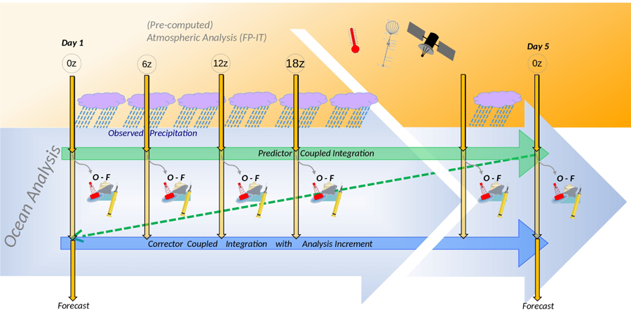
Schematic of Coupled Data Assimilation Methodology. The GEOS-S2S-2 AODAS includes an ocean predictor segment (the green line across the top of the figure), and a corrector segment (blue arrow across the bottom). During both segments the atmosphere is “replayed” to a pre-exisiting atmospheric analysis state every 6 hours (downward yellow arrows). After the 5-day predictor segment, the ocean analysis increments are computed and the coupled AODAS returns to the beginning of the 5-day segment to perform the corrector segment.
Throughout the predictor and corrector steps (depicted in Figure 1), as the coupled atmosphere-ocean model is integrated in time, the sea surface temperature (SST) is strongly relaxed (with a 1-day relaxation time-scale) to the MERRA-2 SST (also used in FPIT) so that the simulated atmosphere in this coupled system is as consistent as possible with the FPIT atmospheric reanalysis. It should be noted that the present GEOS-S2S-2 system has no relaxation to salinity. As the predictor segment proceeds, every 6-hours the departure of the model trajectory (i.e., background field) from observations is gathered, via the so-called ocean observers. Using the background and monthly averaged anomalies of 20 freely-run AOGCMs (with 0.5° × 0.5° × 40 level resolution and no assimilation), we generate ensemble members that are centered about the current background state. The ocean observers are run for all the ensemble members, resulting in an ensemble of innovations (i.e., an ensemble of the departure of observations minus the ensemble member). These innovations combined with the above calculated ensemble members are then used to perform an LETKF analysis. Sea ice fraction (AICE) is replaced by concentrations calculated using the NASA Team algorithm [Cavalieri et al., 1996; Maslanik and Stroeve, 1999] at the analysis step in order to provide optimal ice fields. The coupled model is then rewound to the start of the assimilation cycle to perform the corrector step, during which time the ocean temperature and salinity increments are evenly applied to the ocean trajectory over the first 18 hours of the corrector step to reduce any shocks to the system. The coupled system is then allowed to evolve constrained by FPIT forcing for the remainder of the 5-day segment. This process is then repeated over the next 5-day data assimilation window, cycling over time.
2.2.2. Ocean Data Analysis Technique
The Ocean Analysis used by the GEOS-S2S-2 system follows the Local Ensemble Transform Kalman Filter (LETKF) developed by Penny et al [2013] for ocean applications. Unlike Penny et al [2013], GEOS-S2S-2 ensemble members are derived from an existing trajectory of a free-running coupled model. Thus, in this regard, the GEOS-S2S-2 version of the analysis procedure more closely resembles the Ensemble Optimal Interpolation (EnOI, e.g., Keppenne et al. [2008], Karspeck et al. [2013], Vernieres et al. [2012]). However, the GEOS-S2S-2 ODAS closely matches the LETKF in its other aspects such as the localized influence of any observation on the analysis. More details regarding the LETKF can be found in Ott et al. [2004], Hunt et al. [2007], and Penny et al. [2015].
The GEOS-S2S-2 ocean analysis includes an assimilation of various in situ profile observations summarized in Table 1. Tropical Atmosphere/Ocean (TAO), Prediction and Research Moored Array in the Atlantic (PIRATA), and Research Moored Array for African-Asian-Australian Monsoon Analysis(RAMA) are all fixed tropical mooring arrays that are designed to observe temperature and salinity at depth within the oceanic waveguide [McPhaden et al., 2010] in the Pacific, Atlantic and Indian Oceans, respectively. Expendable Bathythermograph (XBT) data are instruments released from research cruises or volunteer observing ships and so are generally found in regions of repeat transects. Unlike most of the other profile data, XBT data typically only include temperature observations. Conductivity, temperature, and depth (CTD) data are collected by cast from research cruises so are also generally sparse in nature. The major profile data source is from the Argo array [Roemmich et al., 2009]. The Argo array consists of thousands of autonomous profiling Lagrangian floats that descend and ascend through the water column on a regular schedule (typically 10 days, 5m – 2000m), recording temperature, salinity and pressure observations as they travel. When the float surfaces, it transmits the data to the Global Telecommunications System and is made available near-real-time.
Table 1.
Table showing the estimated instrument error, period and source for all data used in the ODAS. The altimeter products were produced by SSALTO/DUACS and distributed by AVISO, with support from CNES (http://www.aviso.altimetry.fr/duacs/).
| Instrument | Inst. Error | Data Coverage | Source | ||||
|---|---|---|---|---|---|---|---|
| T [°C] | S [psu] | SLA [m] | Start | End | Availability/Repeat | ||
| In situ | |||||||
| TAO | 0.02 | 0.1 | 1980 | Present | Daily | PMEL | |
| PIRATA | 0.02 | 0.1 | 1997 | Present | Daily | PMEL | |
| RAMA | 0.09 | 0.1 | 2005 | Present | Daily | PMEL | |
| XBT | 0.1 | 0.1 | Prior to 1980 | Present – 1 month | Sparse –VOS/SOO or research | UK MetOffice | |
| CTD | 0.003 | 0.02 | Prior to 1980 | Present – 1 month | Sparce – research (high vertical resolution) | UK MetOffice | |
| ARGO | 0.005 | 0.02 | 1996 | Present | 10-day cycle – lagrangian | US GODAE | |
| Satellite | |||||||
| Topex | 0.02 | 25-Sep 92 | 24-Apr 02 | 10 day repeat | Copernicus | ||
| ERS-1+2 | 0.02 | 23-Oct 92 | 8-Oct 02 | 35-day repeat | Copernicus | ||
| Geosat FO | 0.02 | 7-Jan 00 | 7-Sep 08 | 17-day repeat | Copernicus | ||
| Jason 1 | 0.02 | 24-Apr 02 | 19-Oct 08 | 10-day repeat | Copernicus | ||
| Jason 2 | 0.02 | 19-Oct 08 | 12-Sep 16 | 10-day repeat | Copernicus | ||
| Jason 3 | 0.02 | 22-Aug 16 | Present | 10-day repeat | Copernicus | ||
| Envisat | 0.02 | 26-Oct 10 | 8-Apr 12 | 35-day repeat | Copernicus | ||
| Cryosat-2 | 0.02 | 28-Jan 11 | Present | 369-day repeat; 3-, 29-, 85-day sub-repeat | Copernicus | ||
| Saral | 0.02 | 14-Mar 13 | Present | 35-day repeat | Copernicus | ||
| HY-2A | 0.02 | 12-Apr 14 | Present | 14-day repeat | Copernicus | ||
| Sentinal 3A | 0.02 | 29-Feb 16 | Present | 27-day repeat | Copernicus | ||
Prior to assimilation into the ODAS, quality control and thinning to limit the data volume are performed on all profile observations. All profile data types are treated in the same way. First each profile is thinned to each model layer by simply averaging all the profile information within a model layer and these data are then assigned to the model layer’s mid-depth. Next, the for quality control, the resulting data are compared against a climatology formulated using all available in situ observations from the World Ocean Atlas 2013 for temperature [Locarnini et al., 2013] and for salinity [Zweng et al., 2013]. Profile data are flagged for poor quality if the observation is more than 6 standard deviations away from the corresponding observation climatology. For the LETKF analysis, data are assigned observational error depending on the depth gradient of the observation. For the GEOS-S2S-2 ODAS, when dT/dz and dS/dz values are greater than or equal to 1.e−3 °C/m and psu/m, respectively, they are scaled by a factor determined by a series of sensitivity studies performed to give the optimal profile observation error. In this way the observational error is greatest at the depth of maximum gradient such as within the thermocline. As a final large-scale error test, any observation with background departure greater than 10° C for temperature and 10 psu for salinity are rejected and not used in the ODAS.
In addition to in situ observations, surface topography observations from satellite altimetry are assimilated in the GEOS-S2S-2 ODAS, which have been utilized to help determine the general ocean circulation, to study seasonal to decadal changes, and to improve global ocean and coupled model initialization. Sea level anomaly is defined as the sea surface height above a mean sea surface (MSS) that is defined over many repeat tracks and independently for each satellite [AVISO, 2013b]. The absolute dynamic topography (ADT) is then the sea level anomaly added to the mean dynamic topography (MDT) which is calculated using a combination of gravity missions (GOCE, GRACE), all available altimetry, and in situ data over the period 1993–2012 [AVISO, 2013c]. Since TOPEX/Poseidon launched in 1992, a series of altimeters have continuously provided ADT observations with varying estimated accuracy of 4 cm [Shum et al., 1995]. Typically the joint US/French series (TOPEX, Jason 1, 2, and 3) have repeat orbits designed to measure the complete globe every 10 days. In contrast, the European satellites have 35-day exact repeat orbits (see Table 1 for details).
A unique aspect of the GEOS-S2S-2 ODAS is the assimilation of absolute dynamic topography (ADT) using the same schedule/technique as is used for the in situ data. Due to the large volume of data, ADT data are ‘thinned’ along track prior to assimilation. A Gaussian weighted mean is calculated for the central point of +/− 10 along-track observations using a decorrelation scale of 1000 km. This weighted mean is then used for assimilation. The observational error for assimilation for this point is the Gaussian-weighted standard deviation of the +/− 10 surrounding along-track points about the mean. The ADT observational error is minimized to 0.1 m and an additional term is added to increase the ADT observational error away from the equator that is proportional to the Rossby deformation radius. This term linearly rises from 0.0 m at the equator to 0.1 m at 90° and the resulting observation error is then scaled by a factor that was tuned to produce optimal fields. The mean of all ADT observations for the assimilation period is removed prior to assimilation and then this mean is added back after assimilation to prevent the sea level from affecting the time-mean barotropic solution. The horizontal localization is identical to that used for the profile data described above. Finally, if any ADT observation departure from mean background is greater than 1.0 m then the observation is removed from consideration.
The LETKF solves the analysis states in a local volume centered on each model grid point and is applied on a regular grid (0.5°x 0.5°x 40 levels). In the GEOS-S2S-2 formulation of the LETKF, the vertical localization is turned off for profile data. This has the benefit of allowing the analysis to be performed only once (as opposed to 40 times), and unlike the previous ODAS system [Vernieres et al., 2012], unique vertical localization profiles for each observation type are no longer applied. This technique has the additional benefit of allowing assimilation of vertical profiles and satellite altimetry data within a single process. The horizontal localization function is used to scale the observational errors such that observations nearer the central model point have higher localization weightings. In addition, the horizontal localization function accounts for the larger Rossby radius of deformation near the equator. This radius varies from 240 km near the equator to less than 10 km near the poles [Chelton et al., 1998]. In practice, the horizontal localization function is parameterized as a Gaussian and as a function of latitude with 1 standard deviation of 3.6 at the equator and 1.8 at the poles. Thus, the impact degrades as the observation point is further from the central point and as the observation latitude increases.
There are many differences between the ocean analysis methods in the GEOS-S2S-1 Borovikov et al. [2017] and GEOS-S2S-2 systems. The major differences are summarized in Table 2. For the current system, initial conditions and verification for the land and atmosphere are provided by the NASA FPIT reanalysis, the GMAO’s near-real-time reanalysis similar to MERRA-2. In GEOS-S2S-2 the observations are incorporated into the ocean state using a 5-day assimilation cycle and the Local Ensemble Transform Kalman Filter (LETKF) using 20 ensemble members (Vernieres et al. [2012]). The advantage of this ensemble Kalman Filter over a less expensive deterministic filter such as the GEOS-S2S-1 SAFE/EnOI (Keppenne et al. [2014], Oke et al. [2010]) techniques is that it allows the error covariances to evolve with the seasonal cycle and the phase of the El Niño Southern Oscillation (ENSO). Another clear advantage of the current system is that GEOS S2S-2 assimilates all available satellite altimetry whereas the previous system did not assimilate any sea level data. In section 4 some key metrics are shown documenting improvements in the current (GEOS-S2S-2) versus the old production system (GEOS-S2S-1).
Table 2.
Table highlighting the differences between the setup for the S2S-v1 (middle column) versus GEOS S2S-2 (right column).
| Component | GEOS-S2S-1 | GEOS-S2S-2 |
|---|---|---|
| Atmosphere | Pre-MERRA-2 version, 1°, 72 vertical levels | Post-MERRA-2 version, 0.5°, 72 vertical levels |
| Ocean / Sea Ice Model | MOM4.1, 0.5°, 40 layers down to 4500m depth, CICE 4.0 | MOM5.0, 0.5°, 40 layers down to 4500m depth, CICE 4.0 |
| Assimilation Technique | SAFE/EnOI, 5-day IAU | LETKF, 18-hr IAU |
| Forecast Error | Pre-specified static forecast error cov. from leading EOFs of an ensemble of forecast anoms. (wrt climate drift) from AOGCM | Estimate evolving errors using monthly-averaged anoms. from 20 freely coupled AOGCMs re-centered about analysis |
| Data | 10-day window, binned to model level, reject if > 6σ from WOA09, obs. error prescribed to observation and type, decorrelation scales x, y, z, t function of variable, unique vertical localization factors applied for each observation and type | 5-day window, binned to model level, reject if > 6σ from WOA13, obs. error from or, horizontal location applied ∝ Rossby deform. radius, no vertical localization applied |
| Assimilation Sequence | Tz, Sz Clim (SAFE) SSS Clim (SAFE) SST (SAFE) Tz (EnOI) Sz (EnOI) AICE |
Tz, Sz, ADT |
| Relaxation Vars | None | SST (1-day), AICE (insertion) |
| Replay Forcing | MERRA corrected using GPCP (< Sep 09), CMAP (Sep 09 - present) | “MERRA-2 like” (FPIT) corrected using CMAP precip. |
2.3. Experiments and Initialization Method
In this study, we examine the results of four sets of seasonal and subseasonal forecasts using the new GEOS-S2S-2 system, a long-term free running simulation with the GEOS-S2S-2 AOGCM, and the GEOS-S2S-2 AODAS reanalysis. The four sets of forecasts are: 1) near-real-time seasonal forecasts (near-real-time means one to two days behind real time), 2) retrospective seasonal forecasts, 3) near-real-time subseasonal forecasts, and 4) retrospective subseasonal forecasts. The long-term simulation is a 50-year long atmosphere-ocean coupled climate simulation with GEOS-S2S-2, which is a “perpetual 2000” simulation, where the external climate forcing is fixed at that of year 2000. For the purpose of a model for seasonal prediction, the 50-year long simulation is adequate to establish an equillibrium climatology down to the depth of the ocean relevant for seasonal forecasts. GEOS-S2S-2 is also utilized in producing an ocean reanalysis (2012-present), that is used to initialize the seasonal and subseasonal near-real-time forecasts. All the simulations, as well as the AODAS, were run at a horizontal resolution of approximately 0.5° longitude and 0.5° latitude in both the atmosphere and ocean components.
In the GEOS-S2S-2, the ensemble of experiments for the retrospective and near-real-time seasonal (and subseasonal) forecasts are handled slightly differently. Historically, for GEOS-S2S-1 and for earlier S2S systems at NASA, owing to the availability of an ocean or a coupled reanalysis state on certain dates only, GMAO forecasts were initialized on a fixed set of calendar dates. These dates begin on Jan 1, and are 5 days apart. In GEOS-S2S-2 we follow the same calendar, and all seasonal forecasts are initialized on the last 4 start dates of the month. For the retrospective seasonal forecasts, no additional ensemble members are generated with perturbed initial states, rather, the start dates form a lagged ensemble of 4 for any month. Seasonal retrospective forecasts were performed for the 36-year period from 1981–2016. Initial conditions for the retrospective seasonal forecasts were generated using a suite of 5-day long coupled data assimilation runs using the GEOS-S2S-2 system, initialized at 5 day intervals from the GEOS-S2S-1 coupled reanalysis initial states.
For near-real-time seasonal forecasts, initial conditions are obtained from a continuous near-real-time GEOS-S2S-2 AODAS reanalysis initialized in 2012 with GEOS-S2S-1 initial conditions. An additional 6 ensemble members are generated around the last start date in each month, thus producing a total of 10 ensemble members (4 unperturbed and 6 perturbed) for each month with this ‘lagged-burst’ strategy. The method to perturb initial conditions is based on the difference between two analysis states 5 days apart. The perturbations are re-scaled and the magnitude of the norm reduced to approximately 10% of the natural variability of SST over the norm region. The rescaling norm is the root mean squared (RMS) difference of the instantaneous sea surface temperatures (SSTs) from two analyses 5 days apart, and the region for defining the norm is the tropical Pacific domain over 120°W-90°W, and 10°S-10°N. The variables perturbed on the ocean model grid are: 3D temperature, salinity and ocean velocities, surface temperature, sea level, ice velocity and strain components, ice strength and stress tensor components, the variables perturbed on the atmospheric grid are: wind components, potential temperature and specific humidity, and the variables perturbed on the free-form ‘tile grid’ used to compute the surface fluxes are: skin temperature, skin layer salinity and skin layer depth. Both the near-real-time forecasts and retrospective forecasts are run for a period of 9 months.
The subseasonal retrospective forecasts are performed for the 17 year period from 1999–2015, according to the protocol of NOAA’s SubX experiment [Pegion et al., 2019]. The retrospective forecasts are initialized every 5 days with a total of 73 start dates per year, with 4 ensemble members per start date. Here, one ensemble member uses the unperturbed initial conditions and the remaining three are generated by perturbing the atmospheric initial conditions in horizontal winds, potential temperature and specific humidity. The perturbations are computed as scaled differences (+/− (x-y)/8) between two arbitrary atmospheric states (x, y) taken 1 day apart. A scaling factor of 1/8 is chosen in an attempt to produce perturbations that are of a size consistent with initial errors typically found in numerical weather prediction models. The initial conditions, as for the seasonal retrospective forecasts, are based on a series of 5-day long coupled ocean data assimilation runs. The near-real-time subseasonal forecast calendar and ensemble are conducted in a similar manner to the retrospective forecasts, with initialization in every 5 days, and 4 ensemble members at each start date. Unperturbed initial conditions for the near-real-time subseasonal forecasts are obtained from the GEOS-S2S-2 near-real-time coupled AODAS. Both the near-real-time forecasts and retrospective subseasonal forecasts are run for a period of 45 days.
3. Climate of Coupled Model
3.1. Mean Atmospheric Climate
All forecasts produced with current weather/seasonal/decadal prediction systems contain within them a long term climate drift reflecting a mismatch between the real world’s climate statistics (implicit in the initial conditions) and those of the model. Such drift is examined in detail in Section 5.1. Here we look at the end point of that drift (i.e., the model’s long-term climate) as a first step in establishing the model’s fidelity and suitability for making short-term (sub-seasonal to seasonal) climate predictions, the underlying assumption being that a model exhibiting smaller long-term climate biases will experience less drift and will potentially produce more skillful forecasts [Chang et al., 2019]. The results here are based on a long simulation with the GEOS-S2S-2 coupled model (see Section 2.3), with the previous version of the model (GEOS-S2S-1) serving as a baseline for comparison. We examine the quality of December-January-February (DJF) and June-July-August (JJA) fields of mean circulation, stationary waves, mean wind, and atmospheric transients, as well as corresponding fields of precipitation, net radiation and surface air temperature. The comparisons highlight some of the key improvements in the circulation, hydrological cycle and radiative balance of the model relative to GEOS-S2S-1, point to areas that still need improvement, and also show a few aspects of the climate that see some degradation in the new model.
Two aspects of the atmospheric circulation that are likely critical to achieving more accurate forecasts over North America (a key focus for our prediction efforts) are the winter stationary waves and the summer North Pacific jet. The former, among other things, provides steering for winter storm systems, while the latter acts as a wave guide for Rossby waves impacting the continent on subseasonal time scales (e.g., Schubert et al. [2011]). Panels a) and b) of Figure 2 show that the mean error (relative to MERRA-2) in the DJF stationary waves (as shown by the 300 hPa eddy heights) is substantially reduced in the new model relative to the old model in both hemispheres. The relevant global metric is the spatial standard deviation, and the difference from MERRA-2, as indicated in the figure caption, has been reduced from 33.07 m in Version 1 to 20.85 in Version 2. In terms of spatial structure, the weak boreal winter stationary waves in GEOS-S2S-1 (especially over the North Pacific/North American region, Figure 2a) are now stronger and closer to the observations as indicated by the smaller biases (Figure 2b). The simulated JJA 200 mb zonal winds show a mix of improvement and degradation in GEOS-S2S-2 relative to GEOS-S2S-1 (Figures 2c and 2d). The middle and high latitudes generally show smaller errors for GEOS-S2S-2, reflecting improvements in the middle latitude jets by reducing the underestimate from nearly 6 ms−1 to nearly zero. However, there is now a larger subtropical westerly wind bias (of approximately an additional 4 ms−1) in the new model in both hemispheres, likely reflecting the split Pacific Intratropical Convergence Zone (ITCZ) and excessive precipitation just north of the equator in GEOS-S2S-2 (see below). Despite these subtropical zonal wind biases, there are substantial improvements in the middle and high latitude transients (not shown) that we argue are tied to the above-noted improvements in the middle and high latitude zonal winds. The moisture fluxes (not shown) in particular are much improved throughout most of the globe during JJA, with the new model showing only weak negative biases in most regions, except for a few isolated regions such as over the North Pacific just off the east coast of Asia.
Figure 2.
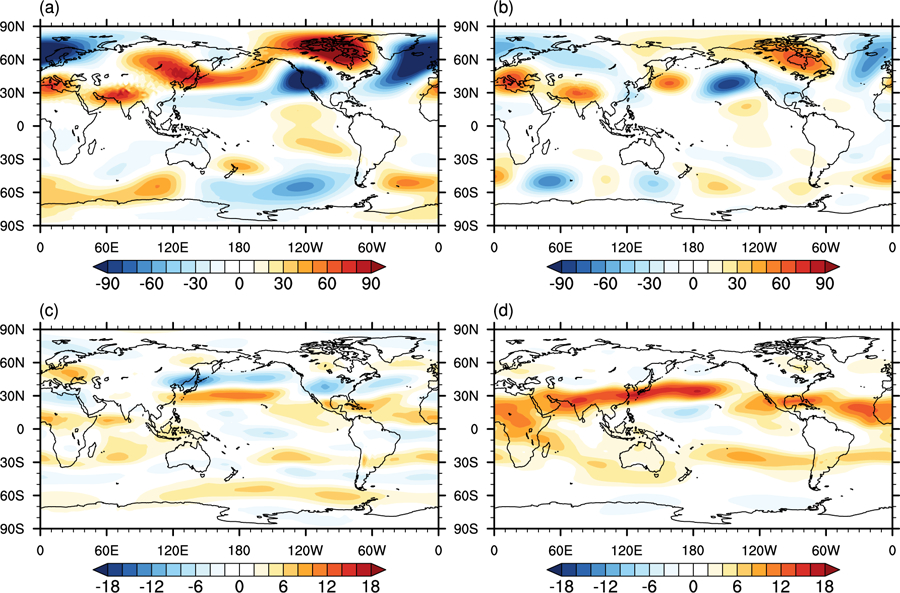
The December-January-February mean eddy height difference from MERRA-2 at 300 mb in m for a) GEOS-S2S-1 and b) GEOS-S2S-2. Global mean difference of spatial standard deviation from MERRA-2 is 33.07 m for GEOS-S2S-1 and 20.85 m for GEOS-S2S-2. The June-July-August mean zonal wind difference from MERRA-2 at 200 mb in ms−1 for c) GEOS-S2S-1, and d) GEOS-S2S-2. Global mean difference from MERRA-2 is 1.0 ms−1 for GEOS-S2S-1 and 2.7 ms−1 for GEOS-S2S-2.
The precipitation biases relative to estimates from the Global Precipitation Climatology Project (GPCP, Huffman et al. [2009]) show a mix of improvements and some degradation in going from GEOS-S2S-1 to GEOS-S2S-2 (Fig. 3). This critical component of the hydrological cycle shows generally reduced biases during DJF in GEOS-S2S-2 (Figure 3c and 3d), including a reduction in the excessive precipitation over the Andes and southern Africa. The main exception is the exacerbation in the new model of positive biases just north of the equator in the Pacific. There is by comparison less improvement in the new model during JJA, especially in the tropics, which is characterized by a much-increased positive bias in the Atlantic and a much more pronounced split ITCZ in the Pacific (Figure 3a and 3b). There is also less rain over India in GEOS-S2S-2, reflecting a weaker summer monsoon rainfall. Important improvements in the new model include the elimination of the excessive precipitation over Tibet and much improved precipitation over the NH storm tracks, presumably reflecting the improved summer transients mentioned earlier.
Figure 3.
Mean total precipitation difference (mm d−1 ) from GPCP, for the GEOS-S2S-1 (a, c) and the GEOS-S2S-2 (b, d). Top panels correspond to the June-July-August season and bottom panels to the December-January-February season. Global mean difference from GPCP in DJF is 0.21 mm d−1 for GEOS-S2S-1 and 0.49 mm d−1 for GEOS-S2S-2, and global mean difference from GPCP in JJA is 0.35 mm d−1 for GEOS-S2S-1 and 0.56 mm d−1 for GEOS-S2S-2.
We evaluate surface air temperature in conjunction with net surface radiation, focusing here on the boreal summer season (though both seasons show substantially reduced biases in both net surface longwave and shortwave radiation, primarily reflecting an overall increased cloudiness). Figure 4 (top panels) shows, relative to estimates from the Surface Radiation Budget (SRB, SRB [2019]) estimates, that the JJA net surface radiation balance is improved overall in GEOS-S2S-2, especially over Asia and North America where the old model had substantial net positive biases of nearly 50 W m−2 and the new model’s bias in those regions is closer to 20 W m−2. These biases apparently contributed to the warm bias in surface temperature over those regions in the old model, as indicated by a comparison of the GEOS-S2S-1 and GEOS-S2S-2 air temperature biases (relative to estimates from Osborn and Jones [2014]) in Figs. 4c and 4d. Substantial positive biases in the net surface radiation balance remain, however, especially over a large region extending from northern Africa eastward across southern Asia and over much of the Indian Ocean north of the equator (Fig. 4c). Of course, not all of the surface temperature biases can be directly related to radiation imbalances. For example, the warm temperatures in GEOS-S2S-2 over India (Fig. 4d) are presumably tied to increases in sensible heat flux associated with a relative lack of rainfall in that region (Fig. 3).
Figure 4.
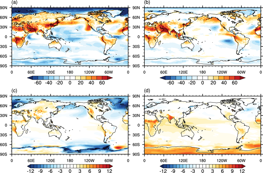
a) June-July-August (JJA) net surface radiation difference (W m−2) from SRB data for GEOS-S2S-1, b) same as a) but for GEOS-S2S-2. Global mean difference from SRB is 0.22 W m−2 for GEOS-S2S-1 and 4.1 W m−2 for GEOS-S2S-2. c) JJA mean 2 m temperature difference from MERRA-2 in °K for GEOS-S2S-1, d) same as c) but for GEOS-S2S-2. Global mean difference from MERRA-2 is −0.85 °K for GEOS-S2S-1 and 0.14 °K for GEOS-S2S-2.
In summary, the biases in GEOS-S2S-2 are generally much reduced throughout the middle and high latitudes, both for the dynamical quantities considered here and for the precipitation, net radiation and surface temperature. The main problems, including the excessive subtropical westerlies and the associated exceptionally warm upper tropospheric temperatures in the tropics (not shown), appear to be linked to excessive tropical precipitation. It is noteworthy that the tropical precipitation biases (and weak precipitation over India) are much reduced, if not absent, from GEOS-S2S-2 simulations when it is run uncoupled from the ocean (i.e., forced with observed SSTs), indicating that these errors are associated with coupled processes. Thus, to understand the nature of these biases, we must also look at the model’s ocean climate. This is the subject of the next subsection.
3.2. Mean Ocean Climate
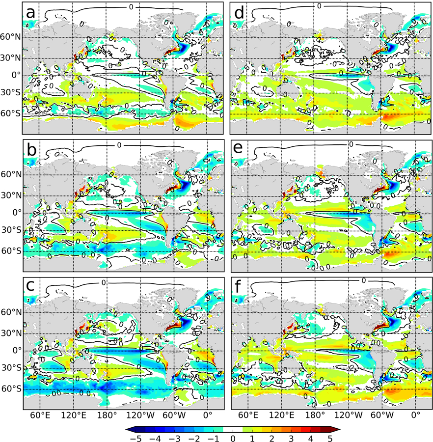
The long term mean climate of the AOGCM is evaluated with observationally-based estimates of various oceanic fields. For example, Figure 5 compares the GEOS-S2S-1 and GEOS-S2S-2 long-term mean sea surface temperature (SST) biases relative to the Reynolds SST analysis [Reynolds et al., 2007]. GEOS-S2S-1 shows strong latitudinally-varying biases (Fig. 5a), with SSTs that are anomalously cool by 2–5 °C or more poleward of 15° North and South. These biases are notably large in the eastern subpolar North Atlantic, which may be related to the weakness of the northward upper ocean transport in this basin. The GEOS-S2S-2 AOGCM (Fig. 5b) has substantially reduced cold biases in these regions, particularly in the subpolar North Atlantic, where the Version 1 model bias in nearly 10 or more °C and the Version 2 model bias is closer to 3 °C, suggesting a more robust overturning circulation (see below). In contrast, in the tropics, the old model’s SSTs are generally too warm, with the highest biases occurring in the near-coastal southeastern Pacific and Atlantic basins. These near-coastal zones are normally cooled by the northward transport of cool water from the southern ocean combining with water being upwelled locally in response to the southerly component of the coastal winds. Low level stratus clouds forming over this cool water further reduces the heat input to the ocean mixed layer. The GEOS-S2S-2 AOGCM (Fig. 5b) has reduced warm biases (from up to 6 °C to less than 4 °C off Africa and near zero off South America) in the near-coastal zones of the southeastern Pacific and Atlantic basins, suggesting that many of these processes have been improved.
Figure 5.
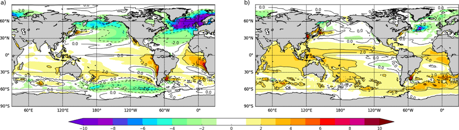
a) GEOS-S2S-1 sea surface temperature difference from Reynolds analysis in °C., b) same as a) but for GEOS-S2S-2. Global mean difference from Reynolds is −0.16 °C for GEOS-S2S-1 and 0.5 °C for GEOS-S2S-2.
The equilibrium state of the cryosphere reflects the behavior of the sea ice model as well as the net radiation and ocean circulation. The equilibrium state of the sea ice extent mean annual cycle in the Northern and Southern hemispheres is shown in Figure 6. Compared to the modern-era satellite measurements [Fetterer et al., 2017], the GEOS-S2S-1 Northern Hemisphere sea ice extent is significantly overestimated over all seasons, consistent with the cold SSTs in the North Atlantic and Pacific sector seen in Figure 5. GEOS-S2S-2 sea ice extent is much improved, especially for late summer and fall. In contrast, the extent in the Southern hemisphere is lower in GEOS-S2S-2 while being much too extensive in austral winter in GEOS-S2S-1. The Southern ocean sea ice bias can also be correlated to SST bias in Figure 5.
Figure 6.
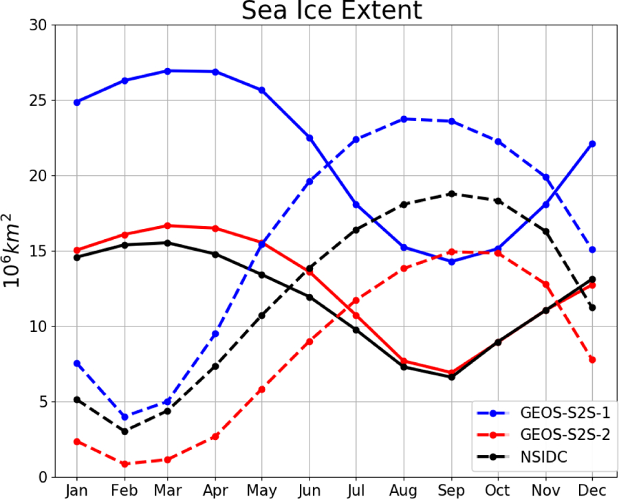
Mean annual cycle of sea ice extent in the Arctic (solid) and Antarctic (dashed). GEOS-S2S-1 (blue) and GEOS-S2S-2 (red) are compared to observational estimates based on passive microwave retrievals (black; NSIDC Sea Ice Index, Fetterer et al. [2017]).
In summary, the mean ocean climate of GEOS-S2S-2 is improved in many ways relative to that of GEOS-S2S-1. Biases in SST, of either sign, are reduced, the phase of the annual cycle is improved, and the evolution of the mean sea ice is improved as well. The Atlantic mean meridional overturning circulation remains weak, however, and the amplitude of the tropical annual cycle is also smaller than that seen in the Reynolds SST dataset. Together, the improvements in the mean bias of both the atmosphere and the ocean states suggest a smaller drift in GEOS-S2S-2, which may hold promise for improvements in forecast skill. The evaluation of the drift and the forecast skill will be presented in Section 5.
4. Ocean Data Assimilation Results - Comparison of S2S-1 and S2S-2
In this section we evaluate the GEOS-S2S-1 and the GEOS-S2S-2 ocean data assimilation system (ODAS) results. The ODAS comparison reflects changes in the model bias and drift as well as the changes in the ocean data assimilation methodology and selection of assimilated fields. In addition, the quality of the ODAS has direct implications for the fidelity of the forecasts that are initialized with the ODAS fields.
For example, the location and amplitude of the western boundary currents have important consequences for longer time scale transport as measured by the global heat and mass transport indices. One such index, the Atlantic Meridional Overturning Circulation (AMOC), is measured by the RAPID array along 26.5°N. The importance of the AMOC for heat transport is clear from the observationally-based AMOC heat transport estimates of Trenberth and Fasullo [2017] of approximately 1 PW. Moorings stretching across the Atlantic at 26.5°N measure temperature, salinity and currents and can thus measure the transport of warm water northward (via the Gulf Stream) and cool water southward (via the North Atlantic deep circulation). The top panel of figure 7 shows that the AMOC for the GEOS-S2S-1 ODAS is consistently weaker than observed. On the other hand, the GEOS-S2S-2 ODAS is initially too strong compared to observed values. However, as the experiment spins down, it settles to match the magnitude of the AMOC in the observations. In addition, the interannual variability of the GEOS-S2S-2 ODAS looks more realistic with respect to observed values as compared to the GEOS-S2S-1 ODAS.
Figure 7.
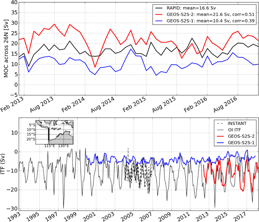
Major global heat transport indices, top) the Atlantic Meridional Overturning circulation (AMOC) is measured by in situ observations of the RAPID array (black) across 26:5° N in the Atlantic. GEOS-S2S-1 (blue) and GEOS-S2S-2 (red) are compared from July 2012 until December 2016. The bottom panel shows indices of the Indonesian Throughflow (see inset for location). Geostrophic transport calculated using an optimal interpolation (Carton [1989]) of all available in situ temperature and salinity observations (solid red) compares well with in measurements from INSTANT moorings Sprintall et al. [2009] (dashed black). GEOS-S2S-1 (blue line) clearly underestimates the ITF transport whereas GEOS-S2S-2 (red line) corresponds well with observations.
Another major region of western boundary current transport related to the global heat transport is the Indonesian Throughflow (ITF). Warm, fresh water is transported through the ITF due to a consistent pressure head from the Pacific to the Indian Ocean. The ITF is important to the global climate system since it moves roughly 15 Sv of warm, fresh water from the Pacific (Sprintall et al. [2009]) and thus is a major source of heat for the Indian Ocean and a sink for the Pacific. In addition, the ITF transports roughly 0.4–1.2 PW of heat from the Pacific into the Indian Ocean [England and Huang, 2005] and so is important for the global heat engine. Another compelling reason to demonstrate fidelity of the ITF statistics is that one of the main products of the GEOS-S2S system is the ENSO forecasts, and the ITF plays an important role as a tropical Pacific thermostat.
Eleven moorings were deployed across the entrance (Makassar Strait, Lifamatola Passage but not Halmahera) and exit regions (Lombok, Ombai, and Timor) of the ITF from 2004–2006 and are dispersed to accurately measure each passage’s contribution to the ITF (Sprintall et al. [2009]). Here we calculate an index of the ITF using a gridded optimal interpolation of observed temperature and salinity (Carton [1989]), convert temperature and salinity to dynamic height, and then calculate geostrophic currents. The transport is then estimated the across 114°E between 21°S and 9°S (closely matching the line used by Meyers et al. [1995]). The good correspondence between the INSTANT measurements (black dashed line in the bottom panel of Figure 7) and our observed ITF estimates (black solid line) demonstrates the fidelity of this technique. The bottom panel of Figure 7 shows that the GEOS-S2S-1 ODAS badly underestimates the transport of the ITF. The mean for GEOS-S2S-1 is approximately −5 Sv whereas observed values are estimated at −15 Sv (INSTANT) and −14 Sv by Wijffels et al. [2008] using QuikScat winds and the Island Rule of Godfrey [1989]. The GEOS-S2S-2 ODAS, in contrast, closely matches the mean, seasonal cycle, and the interannual variability of the observations. The ITF transport of GEOS-S2S-2 clearly outperforms the GEOS-S2S-1 values.
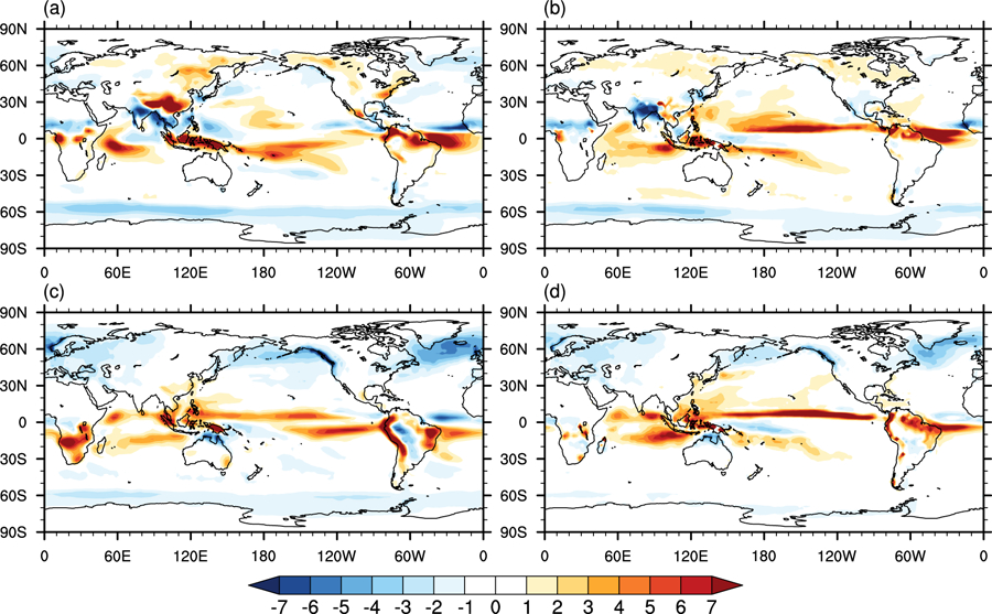
Finally we assess the differences between the GEOS-S2S-1 and GEOS-S2S-2 simulation of the large-scale oceanic Kelvin and Rossby waves in the equatorial Pacific. These waves are instrumental in properly capturing the buildup and recharge stages of ENSO (e.g. Jin [1997]). The ODAS and observed sea level fields are first converted to geostrophic currents (Picaut and Tournier [1991]) then the Kelvin and Rossby amplitudes are calculated using the technique of Delcroix et al. [1994]. The top left panel of Figure 8 shows the observed west-to-east propagating Kelvin wave signal for 2013–2015. Early in the time series, negative (blue) Kelvin waves represent the upwelling associated with the weak 2013 La Niña. The downwelling (red) signals of the 2015 El Niño are evident starting from January 2015 and each successive Kelvin wave increases in magnitude as the Bjerknes feedback becomes enhanced throughout the buildup of this big event (see e.g. Santoso et al. [2015] for details of this event). The amplitude and timing of these Kelvin waves are well reproduced by the GEOS-S2S-2 ODAS (top right panel). On the other hand, the GEOS-S2S-1 shows a generally weaker Kelvin wave amplitude throughout the period (top middle panel). For example, the large Kelvin wave in the summer of 2015 is roughly 30% smaller in the GEOS S2S-1 than in GEOS S2S-2. For the Rossby waves (Figure 8 bottom panels), the lack of amplitude in GEOS S2S-1 is even more evident. The large upwelling (downwelling) Rossby wave in early 2013 (2015) is accurately reproduced by the GEOS-S2S-2 system (bottom right) whereas the GEOS-S2S-1 ODAS badly underestimates these signals. For example, the upwelling in the spring of 2013 reaches −0.3 ms−1 for observations and GEOS-S2S-2 but the GEOS-S2S-1 only peaks at −0.15 ms−1.
Figure 8.
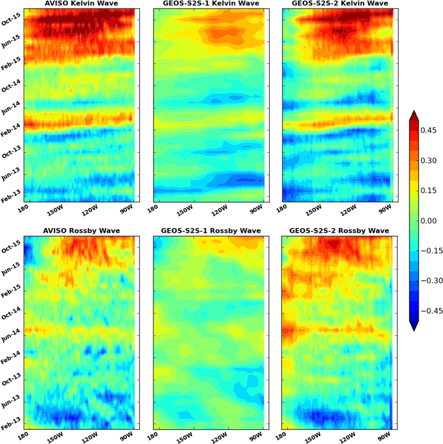
Longitude versus time distribution of the equatorial (top) Kelvin and (bottom) the first meridional mode of equatorial Rossby waves through their signature in zonal surface current deduced from the observed AVISO multi-satellite altimetry AVISO [2013a] (left), GEOS-S2S-1 (middle) and GEOS-S2S-2 (right). Kelvin waves travel west-to-east and take about 3 months to transit the Pacific and Rossby waves travel from east-to-west and take about 8 months.
In summary, almost all ocean variables examined were improved for the GEOS S2S-2 relative to GEOS-S2S-1. SST and SSS biases were reduced (especially off the equator and in the North Atlantic, respectively) but SSS was somewhat degraded over Indonesia and the Amazon plume. Assimilation of Sea Level in GEOS S2S-2 improved the western boundary currents. For example, the large scale meridional (AMOC) and zonal (ITF) heat transport indices were significantly improved in GEOS-S2S-2. The amplitude of the Large-scale Kelvin and Rossby waves were simulated well with GEOS-S2S-2 whereas GEOS-S2S-1 badly underestimated the El Niño and La Niña forcing. Improvements are most likely due to sea level assimilation and better atmospheric assimilation (MERRA-2 versus MERRA) for GEOS-S2S-2 as compared to GEOS-S2S-1.
5. Seasonal and Subseasonal Forecast Assessment
Results of the suite of retrospective subseasonal and seasonal forecasts described in Section 2.3 will be presented here, with a focus on the deterministic measures involving the ensemble mean such as anomaly correlation, root mean square error, and phenomena-based compositing. While forecast assessment should in general include both a deterministic and probabilistic evaluation, the relatively small ensemble size of our seasonal retrospective forecasts limits what we can do to assess the quality of the ensemble (e.g., reliability diagram, Brier skill score). We do, however, provide an initial assessment of the ensemble spread compared to that of the previous system. We begin with a look at the climate drift, keeping in mind that the forecast skill evaluation is performed on the anomalies (after removing the climate drift).
5.1. Climate Drift
In order to provide optimal forecast skill on subseasonal to seasonal time scales, forecast fields are generally calibrated in some way to account for the model drift [Kirtman et al., 2014]. The GEOS-S2S-1 and GEOS-S2S-2 systems follow the convention of Stockdale [1997] and others and calibrates the forecasts by subtracting the drift, computed as the average of the retrospective forecasts. As described in Section 2.3, for GEOS S2S-2 a single retrospective forecast was conducted on each date, while for GEOS S2S-1 multiple forecasts with perturbed initial conditions were conducted [Borovikov et al., 2017]. For the comparison of forecast drift and evaluation of forecast skill, only the unperturbed retrospective forecasts (4 per month) were used from both systems.
Figure 9 shows the DJF seasonal mean error of SST at 1, 3 and 6 month leads. In general, the 1-month lead error is of comparable magnitude in the forecasts with the new and old model (top panels in figure). At 3-month lead time, the GEOS S2S-2 error is close to leveling-off, as seen by the similarity among the 3-month lead error, the 6-month lead error (panels d and f, respectively) and the mean error from the perpetual simulation shown in Figure 5. The GEOS-S2S-1 error, in contrast, continues to grow from 3-month lead to 6-month lead, and has not yet reached the error seen in the equillibrium state of the coupled model. In terms of the drift in the tropical Pacific, the Niño3, Niño3.4 and Niño4 regions show the same behavior as the SST in other regions, with comparable drift at 1-month lead, coming to equilibrium for GEOS S2S-2 at 3-month lead and continuing to grow in GEOS S2S-1.
Figure 9.
a) GEOS-S2S-1 seasonal mean SST drift at 1 month lead time, b) same as a) but at 3 month lead time, c) same as a) but for 6 month lead time, d), e) f) same as a), b), c), respectively for GEOS-S2S-2.
5.2. Forecast skill at subseasonal time scales: MJO and Stratospheric Warmings
The Madden-Julian oscillation (MJO) is the dominant mode of tropical intraseasonal variability and provides a major source of tropical and extratropical predictability on sub-seasonal time scales (eg., Waliser et al. [2003]). The prediction skill, therefore, of the MJO, is a critical indicator of subseasonal time scale prediction skill. Figure 10b shows the correlation between the bivariate Real-time Multivariate MJO (RMM) index from the suite of GEOS-S2S-2 retrospective forecasts described in Section 2.3 and MERRA-2 [GMAO, 2015] as a function of the forecast lead. Figure 10a shows the same field but from the GEOS-S2S-1 suite of retrospective forecasts described in Borovikov et al. [2017]. The RMM index is derived from the zonal wind at 850hPa and 200hPa and outgoing longwave radiation following the method described in Wheeler and Hendon [2004] and Gottschalck et al. [2010].
Figure 10.
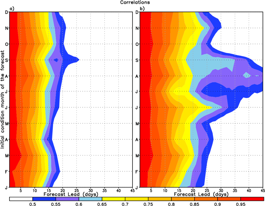
a) Bivariate anomaly correlation of the RMM index as a function of forecast lead day and month of initialization from GEOS-S2S-1, b) same as (a) but for GEOS-S2S-2
The comparison shows that at short lead times (1–10 day lead), the correlation is greater than 0.80–0.85 for all initial condition months for both GEOS-S2S-2 and GEOS-S2S-1. At intermediate leads, up to 25 days, there is a clear improvement in skill in GEOS-S2S-2 relative to GEOS-S2S-1. Prediction skill at long lead time is particularly high in GEOS-S2S-2 for summer initial conditions, exceeding correlations of 0.5 even at 40 day lead. It should be noted that as compared with other current S2S forecasts from other centers (eg., Saha et al. [2014]; Scaife et al. [2016]), GEOS-S2S-2 is among the systems with the highest skill.
Another variation at subseasonal time scales that, under certain circumstances, adds predictability at these time scales is the Sudden Stratospheric Warming (SSW). SSWs are dramatic changes in the wintertime stratospheric circulation where the zonal mean zonal wind westerlies reverse as the temperature increases in the polar night [Butler et al., 2015]. These stratospheric changes are often associated with subsequent changes in tropospheric circulation [Baldwin and Dunkerton, 2001; Kretchmer et al., 2018] implying that skill in forecasting the stratospheric disruptions may aid in long range weather prediction. Here we examine the composite 45-day GEOS-S2S-2 SSW forecasts of stratospheric winds, temperatures, and planetary wave forcing for the Northern Hemisphere (NH) SSW events that occurred during the GEOS-S2S-2 retrospective forecast time period [Butler et al., 2017].
Figure 11 shows the composite over the 15 SSW events along with the corresponding MERRA-2 [GMAO, 2015] composite for validation. The initial times were binned to 5, 10, 15, 20, 25 and 30 days before the SSW dates. The forecasted stratospheric polar temperatures (Fig. 11a) capture the peak warming temperature at 5 and 10 day lead times and follow the main peak closely at 15 day lead time. The longer lead times falter in capturing the SSW temperature peak, however, they all show a warming over climatology. Note that the 5, 10, and 15 lead time curves all track the post SSW cooling closely out to about 20 days after the SSW date. After the SSW date, planetary wave activity is greatly reduced as the westerlies change to easterlies and the stratosphere becomes more predictable. Figure 11b shows the forecast of the zonal wind. The 5, 10, and 15 day lead times show significant reduction in the zonal wind relative to climatology with the 5 day lead time closely tracking the SSW reduction and the subsequent return to climatology. The longer lead times show some reduction in zonal wind, although they remain close to climatological values. Figure 11c shows the 100 hPa meridional heat flux, a standard measure of the tropospheric forcing of the stratospheric waves [Andrews et al., 1987]. The 5 day lead time captures the peak of the heat flux and the following decrease, however the 10 and 15 day lead times reduce the heat flux before the SSW date. These weaker heat fluxes were noted by Karpechko et al. [2018] in their examination of the February 2018 SSW forecasts. All the forecast lead times captured the reduced heat flux, corresponding to reduced planetary wave activity, following the SSW date.
Figure 11.
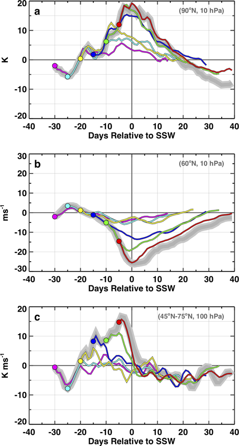
a) Composite temperature in °K for SSW events from MERRA-2 (grey) and from GEOS-S2S-2 forecasts at different lead times: 5-day (red), 10-day (green), 15-day (blue), 20-day (yellow), 25-day (cyan) and 30-day (purple), b) same as a) but for zonal wind in ms−1, c) same as a) but for meridional heat flux in °Kms−1
GEOS-S2S-2 performs well in forecasting the key composite SSW characteristics out to approximately 15 days, consistent with the forecasting results of Tripathi et al. [2016]. These include the increase in polar temperature, the decrease in zonal mean zonal wind, and the decrease in heat flux following the SSW date. The longer than 15 day forecasts perform well in the post SSW period when planetary waves are weak, a key time of interest for changes in tropospheric weather associated with the SSW events. The heat flux may be more difficult to forecast than winds and temperatures as the calculation involves the correlation between winds and temperatures and the zonal mean averages both positive and negative values. More study is needed to asses the skill available for individual events as well as the potential usefulness of GEOS-S2S-2 SSW forecasts that may miss the specific verifying dates used here.
5.3. Forecast skill at seasonal time scales
The dominant mode of variability of the earth system at seasonal time scales is the El Niño/Southern Oscillation (ENSO), and the assessment of GEOS-S2S seasonal forecast skill begins with evaluating ENSO forecasts. ENSO related anomalies impact global atmospheric circulation and modulate tropical cyclone activity, other tropical modes, and many tropical-extratropical teleconnection patterns. To ensure the fidelity of these connections in the seasonal forecasts, the other dominant modes of variability in the tropics and extratropics are also evaluated below, as is the tropical cyclone strength and frequency. To assess the local impact of the atmospheric variability in terms of local metrics that most affect the population, GEOS-S2S skill of surface temperature and precipitation is also evaluated. Finally, given the improved GEOS-S2S-2 model parameterizations related to the cryosphere (see Section 2.1) and the expansion of the earth system simulated to include an interactive aerosol model, we also present here an evaluation of the forecast skill in the cryosphere, and the assessment of forecast skill of the aerosol load.
5.3.1. Skill of Global SST, Niño 3.4
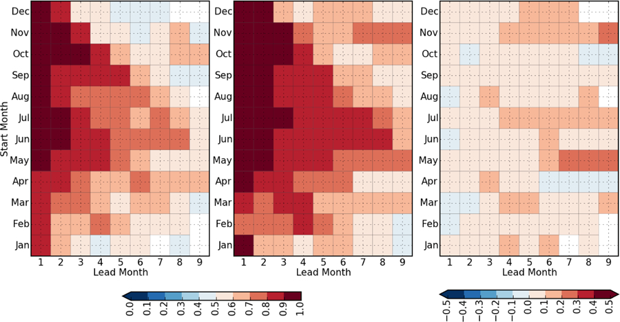
An overview of the prediction skill of ENSO and the comparison of GEOS-S2S-2 and GEOS-S2S-1 is shown in Figures 12 and 13. Figure 12 shows the anomaly correlation of the Niño 3.4 SST index, using Reynolds SST for comparison. In Figure 12c, pink (blue) boxes indicate regions where GEOS-S2S-2 outperforms (degrades) forecasts with respect to GEOS-S2S-1.
Figure 12.
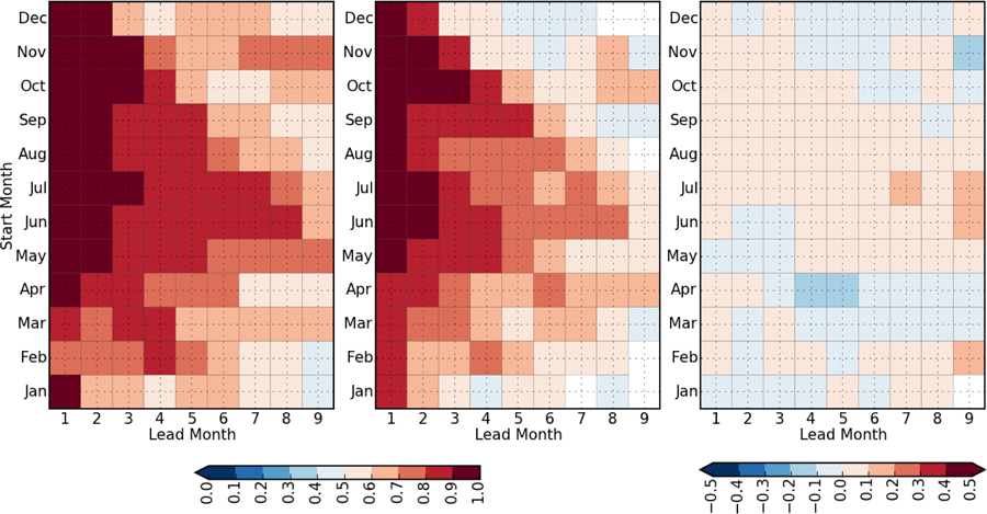
Anomaly correlation for Niño 3.4 SST index. Reynolds SST is used for comparison. Initial forecast month is on the y-axis, lead time on the x-axis. The left panel is GEOS-S2S-1, middle panel GEOS-S2S-1, and the right panel is GEOS-S2S-2 minus GEOS-S2S-1. Positive values indicate an improvement of GEOS-S2S-2 relative to GEOS-S2S-1.
Figure 13.
Same as Figure 12, but for the Niño1+2 index.
The right panel shows a mixture of positive and negative difference in correlation (pink and blue colors, respectively), indicating that the forecast skill in the east-central Pacific in general is comparable in both new and old versions of GEOS S2S. In general, forecasts issued in summer and into the late fall show improved skill in GEOS S2S-2 (pink colors), and forecasts issued in the spring show a degradation (blue). The anomaly correlation of the Niño1+2 index is shown in Figure 13 and is the indicator of SST skill in the eastern Pacific. The rightmost panel shows a clear improvement in GEOS-S2S-2 for almost all lead times and all initial condition dates. The improvement of GEOS-S2S-2 over GEOS-S2S-1 generally increases with forecast lead time, as indicated by the deeper pink shades toward the right side of the figure.
An important additional set of metrics for the seasonal ENSO forecast are the statistical measures of forecast reliability. In part due to the small ensemble size, we present here a measure of the spread among forecasts as it relates to the forecast error. By this measure, a ‘reliable’ forecast is one in which the ensemble spread is large (small) when the error is large (small). That is, the ensemble spread is a reliable indicator of the error. The ratio: R = intra ensemblespread / standard error should ideally be close to 1. Figure 14 shows the R ratio for GEOS-S2S-2 and GEOS-S2S-1. R values less than 1 indicate under-dispersive forecasts, meaning that the forecast is overconfident in a wrong answer. Values greater than 1 indicate less than appropriate confidence in a right answer. The figure shows that GEOS-S2S-1 is under-dispersive (consistent with the finding of Barnston et al. [2015]), especially early in the forecasts and more so for Niño1+2 than for Niño 3.4. In contrast, GEOS-S2S-2 is generally over-dispersive, at long leads, especially for forecasts initialized in boreal summer and early winter. Only at very short leads (1–2 months) is GEOS-S2S-2 still under-dispersive.
Figure 14.
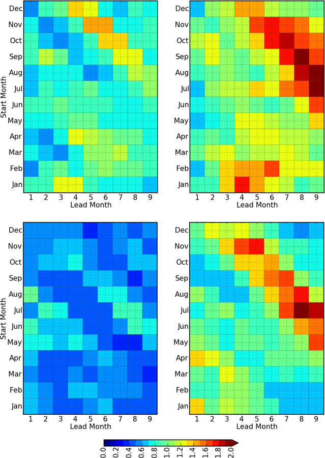
The ratio R (see text), for the Niño 3.4 index (top row) and Niño1+2 index (bottom row) as a function start month and forecast lead time for GEOS-S2S-1 (left) and GEOS-S2S-2 (right). Results are based on four ensemble members for forecasts/hindcasts spanning the period 1982–2016.
5.3.2. Teleconnections and Low Frequency Mode Prediction
The major sources of northern hemisphere extratropical variability and so predictability on seasonal time scales are the North Atlantic Oscillation (NAO, Stephenson et al. [2003]), the Northern Annular Mode/Arctic Oscillation (NAM/AO, Thompson and Wallace [2001]), and the Pacific North American (PNA) pattern [Wallace and Gutzler, 1981]. These major teleconnection patterns for boreal winter are captured by performing a Rotated Empirical Orthogonal Function (REOF) analysis using the 250mb geopotential height field from the MERRA-2 reanalysis. The NAO, AO and PNA are the leading eigenvectors from this analysis. The REOF analysis is repeated using the retrospective seasonal forecasts from GEOS-S2S-2 and GEOS-S2S-1, and both exhibit realistic spatial patterns. Here we assess how reliably the GEOS-S2S systems can predict the phase/intensity of the NAO, PNA and AO. The time series of the teleconnection pattern indices are shown in Figure 15, where we see the interannual variations of the January/February averaged teleconnection indices (initialized on December 27) computed from GEOS-S2S-2, GEOS-S2S-1, and MERRA-2. The teleconnection indices are computed by projecting the anomalous 250mb geopotential height over the Northern Hemisphere onto the spatial REOFs of the teleconnection patterns. Comparison of the indices and the correlations with MERRA-2 demonstrates clearly that GEOS-S2S-2 has improved the forecast skill by achieving anomaly correlations greater than 0.5 for all three teleconnection patterns. The improvements in all three indices are statistically significant.
Figure 15.
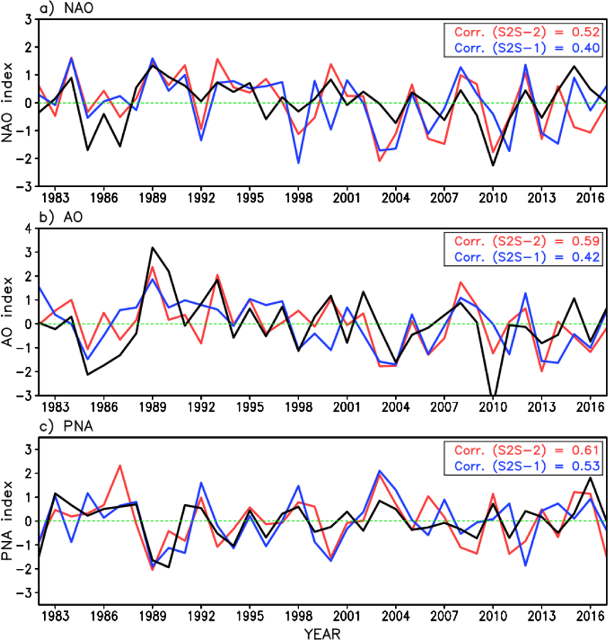
January/February mean NAO (a), AO (b), and PNA (c) teleconnection indices predicted by GEOS S2S-2 (red) and GEOS S2S-1 (blue) initialized on 27 December. The black line represents the MERRA-2 teleconnection indices. Correlations between MERRA-2 and GEOS-S2S-2 (red), and between MERRA-2 and GEOS-S2S-1 (blue), respectively, are shown on the upper-right corner of the each panel.
5.3.3. TC activity
Seasonal forecasts of tropical cyclone activity are widely used for decision making and preparedness. The predictive skill of seasonal tropical cyclone (TC) activity from the GEOS-S2S systems is assessed in terms of the Genesis Potential Index (GPI) [Emanuel and Nolan, 2004], which is an empirically determined function of state variables which influence TC genesis. The GPI is generally larger than normal when TC activity (e.g., counts and intensity) is stronger than usual, and smaller during a weak TC season. We compute the GPI over the North Atlantic and the Western Pacific regions from the GEOS-S2S-2 and GEOS-S2S-1 retrospective forecasts and then compare the interannual variation of the GPI with that computed from MERRA-2. Time series over the period 1982–2016 in Figure 16 show the GPI for each year as the averaged GPI from June through September (initialized on May 31). Both GEOS-S2S-2 and GEOS S2S-1 have the ability to predict TC activity up to four months lead time at the beginning of the TC season. Comparison between GEOS-S2S-2 and GEOS-S2S-1 correlations indicates relatively comparable performance in the Atlantic, but better correlations with MERRA-2 in GEOS-S2S-2 in the Western Pacific.
Figure 16.
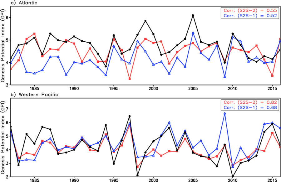
Predicted June/July/August/September (JJAS) genesis potential index (GPI) from forecasts initialized on 31 May. a) North Atlantic region, b) Western Pacific region. Blue, red, and black solid lines denote the results from the GEOS S2S-1, GEOS S2S-2, and MERRA-2, respectively. Correlations between MERRA-2 and GEOS-S2S-2 (red), and between MERRA-2 and GEOS-S2S-1 (blue) are given on the upper-right corner of the each panel.
5.3.4. Skill of T2m and Precip
Near-real-time seasonal forecasts of surface air temperature and precipitation over land are the most widely used products of seasonal prediction systems and the need for reliable forecasts of these fields continues to motivate many national development efforts across the globe. We use the suite of retrospective forecasts from GEOS S2S-2 and GEOS S2S-1 to evaluate the skill of these two critical quantities. Consistent with the reduction in SST bias shown in sections 3 and 5.1, the root mean square error of the surface temperature is improved in GEOS S2S-2 across the board (not shown), and most markedly in boreal winter. The metric that is more challenging and more relevant for the surface temperature and precipitation is the anomaly correlation (AC). In Figure 17, the differences in AC between the two systems are small, but there are notable improvements in GEOS S2S-2. The AC of near-surface temperature is above 0.5 for most regions in both systems for the first lead month (AC itself is not shown) and as can be seen in Figure 17 is improved for northern hemisphere high latitude in Siberia and North America in GEOS-S2S-2 by up to 0.3. Improved skills of up to 0.4 are also seen in South America for all lead times. In general, for both GEOS-S2S-1 and GEOS-S2S-2, AC of near-surface temperature decreases quickly as lead time increases. The decrease of AC with lead time in both systems is slower in JJA as compared to DJF, as indicated by the presence of AC values above 0.5 in many regions even at 7 months lead time (not shown). Precipitation forecasts are a common challenge for most seasonal forecast systems due to complex spatial and temporal variability [Kirtman et al., 2014]. In general, comparing GEOS-S2S-1 and GEOS-S2S-2 (Figure 18), while the changes of AC are not spatially coherent and mixed in sign, improvements of up to 0.3 are found in the western tropical Pacific in the first month lead for JJA and in the Amazon region for longer lead months for DJF.
Figure 17.
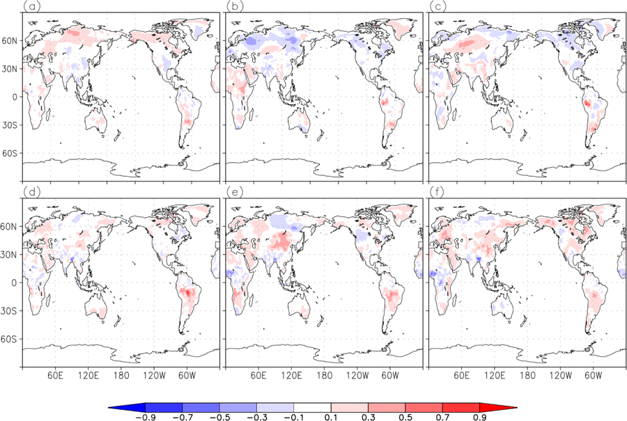
a) JJA Seasonal mean GEOS S2S-2 minus GEOS S2S-1 AC of near-surface temperature at 1-month lead, b) same as a) but for 4-month lead, c) same as a) but for 7-month lead, d) DJF Seasonal mean GEOS S2S-2 minus GEOS S2S-1 AC of near-surface temperature at 1-month lead, e) same as d) but for 4-month lead, f) same as d) but for 7-month lead. Red areas in the difference figure indicate improvement in forecast skill in GEOS-S2S-2 compared to GEOS-S2S-1, and only statistically significant values are shaded.
Figure 18.
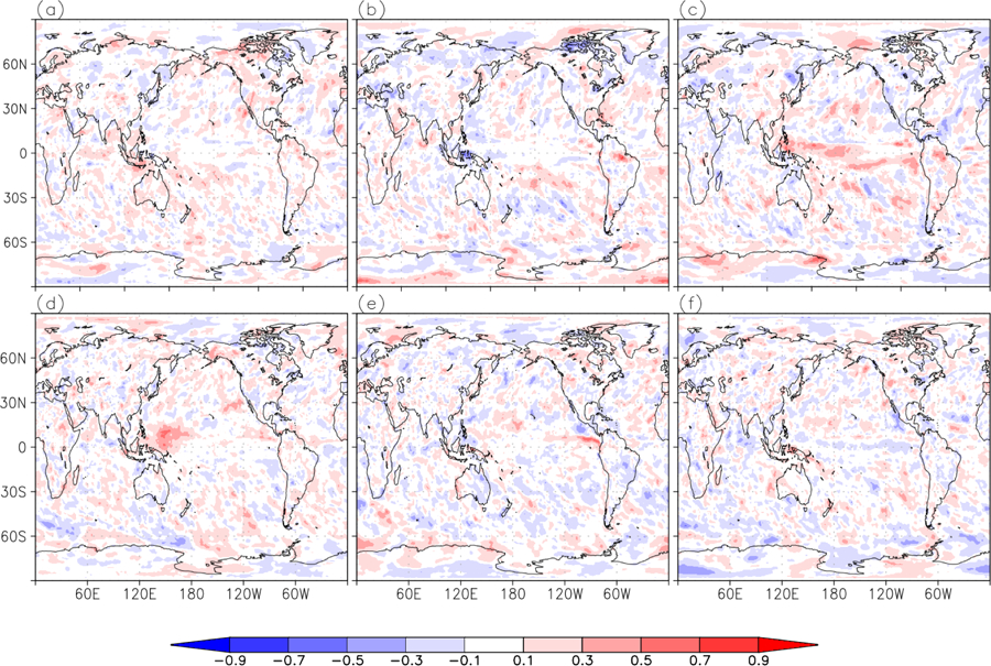
Same as Figure 17 but for precipitation.
5.3.5. Cryosphere
The presence and character of sea ice substantially alters the local energy and moisture exchange between the ocean and atmosphere, affecting the local Arctic and Antarctic climate. In the Arctic, the accelerated reduction of sea ice cover in recent years is also associated with a regional amplification in near-surface air temperatures [Screen and Simmonds, 2010; Serreze and Barry, 2011]. These effects may also influence the larger-scale general circulation [Alexander et al., 2004; Deser et al., 2010; Screen et al., 2018]. Appropriate treatment of sea ice characteristics in seasonal forecasting models may then influence Northern Hemisphere predictive skill [Jung et al., 2014]; however, there is uncertainty in the causal relationship between Arctic sea ice conditions and midlatitude weather variability [Overland et al., 2015], in part due to the limited the atmospheric response to sea ice variability in models [Screen et al., 2018]. Nevertheless, local improvements in sea ice forecasts provide useful information for Arctic stakeholders [Ban et al., 2016].
The GEOS-S2S-1 forecasting system demonstrated reasonable predictive skill of hemispheric sea ice cover [Borovikov et al., 2017], with June forecasts explaining approximately 50 percent of the observed variance in the September Arctic ice extent (Figure 19). In producing GEOS-S2S-2, a key goal was to assess the best predictive skill attainable with the GEOS-S2S-2 model configuration. To this end, forecasts for the retrospective period were initialized with ice thickness values from a validated modeling system (GIOMAS: Global Ice-Ocean Modeling and Assimilation System; Schweiger et al. [2011]). The use of GIOMAS sea ice thicknesses resulted in substantial improvement in forecast skill at longer lead time. The use of GIOMAS and FPIT atmospheric forcing effectively eliminated a large springtime negative sea ice extent bias found in earlier versions of the seasonal prediction system (Figure 19b).
Figure 19.
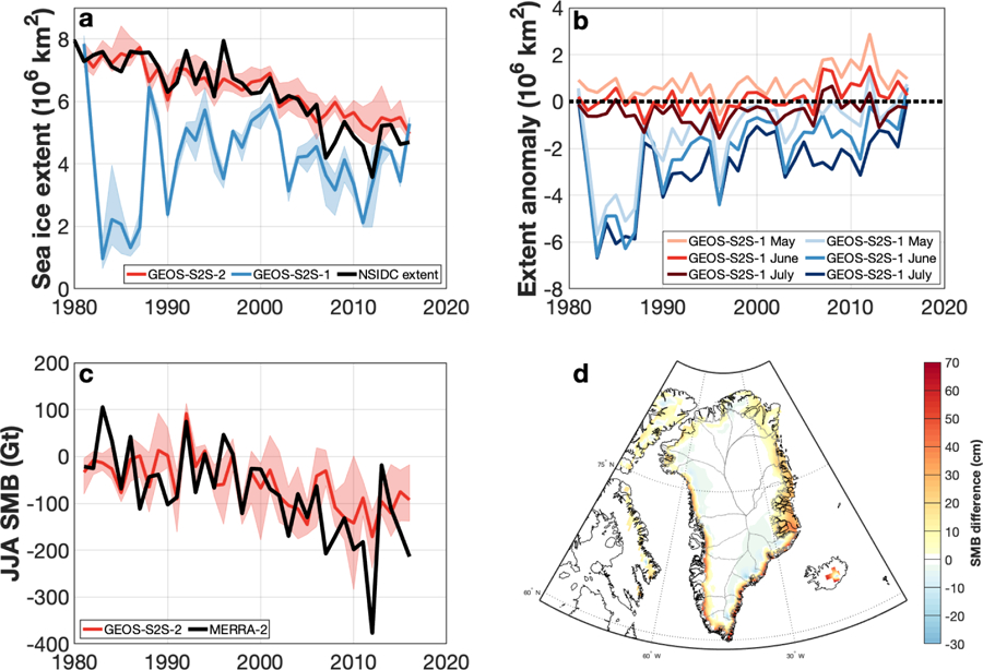
a) June retrospective forecasts of September Northern Hemisphere sea ice extent for GEOS-S2S-2 (ensemble mean, red line; ensemble spread, red shading), GEOS-S2S-1 (ensemble mean, blue line; ensemble spread, blue shading) and sea ice concentrations derived from satellite brightness temperature (black, Cavalieri et al. [1996]). b) May, June, and July retrospective forecast anomalies of GEOS-S2S-2 and GEOS-S2S-1 (as differenced from Cavalieri et al. [1996]) for September Northern Hemisphere sea ice extent. c) Greenland Ice Sheet summer (JJA) surface mass balance from GEOS-S2S-2 June forecasts (ensemble mean, red line; ensemble spread red shading) and MERRA-2 (thick black). d) Mean (1981–2016) Greenland Ice Sheet surface mass balance difference (GEOS-S2S-2 minus MERRA-2). Positive values (red) indicate that GEOS-S2S-2 loses less mass to ice sheet runoff than MERRA-2, and negative values (blue) indicate that GEOS-S2S-2 loses more.
A credible initial ice thickness field has been widely demonstrated to improve the seasonal forecast skill for sea ice extent (e.g., Blanchard-Wrigglesworth et al. [2017]; Chevallier and Salas-Melia [2011]; Day et al. [2014]). Retrospective forecasts of the GEOS-S2S-2 system using GIOMAS are substantially improved over the previous system (Figure 19a, b). But much of this skill is imparted from the long-term trend towards lower ice extent; the detrended retrospective July forecasts (after Bushuk et al. [2012]) explain approximately 30 percent of the observed sea ice extent variability. This reduction in the detrended forecast skill is commonly found in dynamical sea ice forecasting models (e.g., Hamilton and Stroeve [2016]. The results nevertheless highlight the importance of deriving an accurate, historical record of ice thickness and methods for incorporating near-real-time ice thickness observations in future seasonal forecasting systems.
Changes in glacier and ice sheet surface mass balance (SMB: here, the net of precipitation minus evaporation/sublimation and runoff) may alter the climate on seasonal timescales via local changes to surface energy budget characteristics (i.e. ice surface albedo; [Box et al., 2012] and through the selective discharge of freshwater, which may impact local fjord circulation as well as ocean stratification [Mortensen et al., 2013; Sciascia et al., 2013]. The appropriate representation of glacier and ice sheet SMB processes is an important step in improving the complexity of seasonal prediction systems and may provide valuable information to a range of stake holders.
The GEOS-S2S-2 system incorporates the same surface energy and snow hydrology schemes used in MERRA-2 [Cullather et al., 2014]. Fractional snow cover over land ice is explicitly represented with a modified version of the Stieglitz snow model [Lynch-Stieglitz, 1994; Stieglitz et al., 2001]. An underlying 15-layer ice column resolves surface heat conduction, with a lower boundary condition of zero heat flux. Meltwater runoff may occur both from the snow column and bare ice surfaces. This scheme produces a reasonable representation of SMB for the Greenland Ice Sheet (GrIS) when compared to both in situ measurements and high-resolution regional climate models [Cullather et al., 2014], although the reduced spatial resolution may limit the ability to appropriately represent the surface melt spatial extent and gradients within the ablation zone. Nevertheless, the results compare well with localized observations [Smith et al., 2017].
The current forecasting system reasonably reproduces the spatial pattern of mean SMB during the retrospective forecast period at 1-month lead times (1981–2016; 19c, d): regions of high snow accumulation in southeastern GrIS are clearly present. But in general there is an under-prediction of wintertime snow accumulation, and a larger under-prediction in ice sheet runoff, particularly during the latter part of the retrospective forecast period (19d). In this more recent period, summer conditions were generally associated with a strongly negative NAO index. This is characterized by warmer surface air temperatures over the western GrIS [Lim et al., 2016], which is largely absent in the GEOS-S2S-2 forecasts. In these summers associated with a negative NAO index, the under-prediction of ice sheet runoff also corresponds to an overestimate in the predicted summertime sea ice cover at leads of 3–4 months. Localized feedbacks between sea ice extent and ice sheet runoff (e.g., Liu et al. [2016]), initial conditions, and ice sheet surface albedo feedbacks may be factors in summertime SMB forecasting [Box et al., 2012; Tedesco et al., 2013].
Aside from the trend toward reduced skill in the retrospective period, May forecasts are found to predict approximately 66 percent of the total variance of the JJA (lead times of 1–3 months) SMB relative to MERRA-2. As with sea ice cover, much of the skill in forecasting summer SMB arises from the ability to predict the recent trend towards enhanced ice ablation [Khan et al., 2015], and not necessarily the SMB interannual variability.
5.4. Results of Aerosol Forecast
Forecasts of aerosol loading that are possible with GEOS-S2S-2 (see the description of the GOCART interactive aerosol model in section 2.1) are included as part of only a few seasonal prediction systems (eg., Benedetti and Vitart [2018]), none of them operating in near-real-time forecast systems, and interactive aerosols have been shown to improve monthly scale prediction during the spring/summer. Here we use the MERRA-2 aerosol optical depth (AOD) at 550nm [Randles et al., 2017] to evaluate the GEOS-S2S-2 retrospective forecasts of AOD. MERRA-2 includes an aerosol analysis (the Goddard Aerosol Assimilation System, Buchard et al. [2015]; Buchard et al. [2016]) and so will be the basis for evaluation of the forecasts. Our analysis is focused on one-month lead time forecasts of seasonal mean behavior in December, January, and February (DJF), and July, August, and September (JAS) from 2000 to 2015.
Figure 20 shows that the GEOS-S2S-2 aerosol global mean and seasonal spatial distributions are in general agreement with MERRA-2, capturing the main patterns of the biomass burning aerosols over South America, Africa and the South Atlantic Ocean, the position of the dust plume coming from the Sahara desert, and the Asian pollution plume. There are however, errors over a few specific regions (Figure 20c,d). During the Austral winter (JAS) GEOS-S2S-2 overestimates the AOD on the southwestern coast of Africa, India, and in the boreal forest in North America and Asia, and underestimates over South America and southeast Asian, associated with biomass burning emissions. It is noticeable (not shown) that the AOD biases correlate well with the precipitation biases in South America and Africa. Therefore, the GEOS-S2S-2 overestimation and underestimation over Africa and South America, respectively, is likely related to the model ability to predict precipitation accurately, and therefore also to the wet removal processes over these regions. For the same season, GEOS-S2S-2 also overestimates the AOD on the north of Africa and the Middle East, related to dust emissions. The positive AOD biases associated with dust aerosols are related to stronger winds simulated by the GEOS-S2S-2 compared to the meteorological reanalysis. A similar feature and bias have been previously reported for GEOS model results [Textor et al., 2006; Colarco et al, 2010; Randles et al., 2013]. During Boreal winter (DJF), GEOS-S2S-2 overestimates the aerosol loading in the Arctic, and over Central Africa, associated with boreal fires. During DJF the GEOS-S2S-2 prediction underestimated the AOD over India, northern South America, and eastern Asia. The climate prediction of sea-salt aerosols over oceanic regions are typically underestimated both over the Southern and Northern Hemispheres during Austral and Boreal winter. This underestimation is likely related to the prediction of meteorological factors influencing sea-salt emissions, such as wind speed at 10m and the sea surface temperature (SST).
Figure 20.
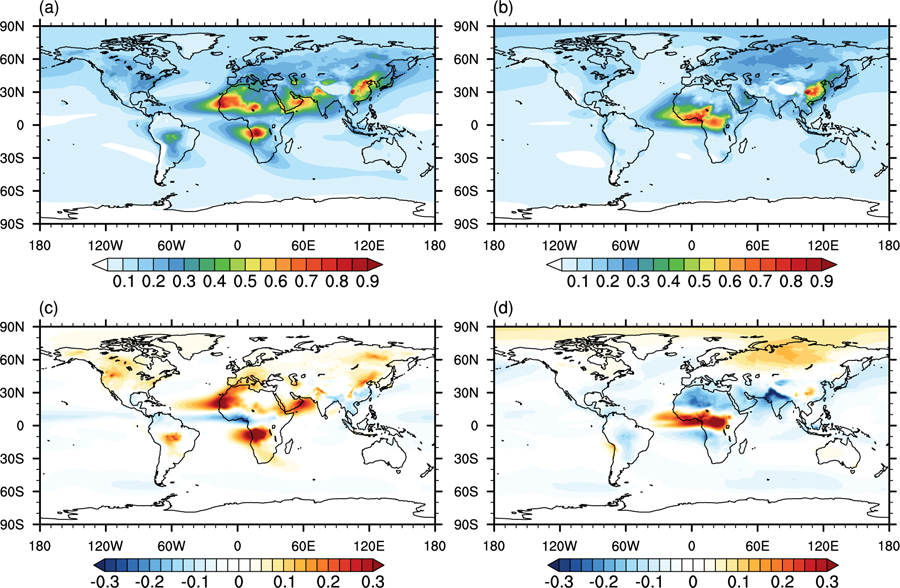
a) Spatial distribution of aerosol optical depth (AOD) at 550 nm in July-August-September and b) December-January-February, averaged for the period 2000–2015 from the GEOS-S2S-2 ensemble mean. c) like a) but GEOS-S2S-2 minus MERRA-2 AOD, d) like b) but GEOS-S2S-2 minus MERRA-2 AOD. Global mean difference from MERRA-2 in JAS is 0.11 and in DJF is −0.05.
6. Summary and Future Directions
We have presented here a detailed description of the Global Modeling and Assimilation Office (GMAO) Global Earth Observing System Subseasonal to Seasonal Prediction System Version 2 (GEOS-S2S-2), along with a detailed evaluation of the climate of the Atmosphere-Ocean General Circulation Model (AOGCM), the coupled Atmosphere-ocean Data Assimilation System (AODAS), and the skill of subseasonal and seasonal forecasts. GEOS S2S Version 2 was released in the fall of 2017 and has been running near-real-time (lagged one or two days behind real time) since then, providing selected output to participate in many community multi-model ensemble projects. GMAO’s S2S Version 3 is due for release at the end of 2019, will be used as the basis for a modern era coupled reanalysis spanning from 1981 to present, and will replace Version 2 when it ‘catches up’ to real time. Some of the issues and shortcomings revealed in the evaluation of GEOS-S2S-2 presented here have been addressed in the Version 3 development process.
The evaluation of the climate or equillibrium state of the atmosphere and ocean of the free-running AOGCM was presented to underscore the importance of quantifying and reducing climate drift, since it represents the state to which the forecast will eventually drift. The climatological biases in the GEOS-S2S-2 AOGCM were in fact shown to be substantially reduced relative to GEOS-S2S-1, with remaining issues related to warm land surface temperatures and excess surface radiation during boreal summer, the ubiquitous ‘double ITCZ’, warm SSTs by up to 2° K over much of the globe, and a weak Atlantic Meridional Overturning circulation. The evaluation GEOS-S2S-2 coupled reanalysis also revealed substantial improvements in GEOS-S2S-2 relative to GEOS-S2S-1, particularly related to the assimilation in the new system of along-track absolute dynamic topography. The improvements include a stronger AMOC, improved heat content, and more robust propagation of Kelvin and Rossby wave signals.
The evaluation of forecast skill found a much-improved prediction of the Madden-Julian Oscillation, now comparable in skill to the community state of the art. Sudden Stratospheric Warmings were also found to be predictable on subseasonal time scales out to 20 days in some cases. An assessment of ENSO forecasts showed that GEOS-S2S-2 is comparable in skill to GEOS-S2S-1 with, however, clear improvements in dispersion characteristics in that the ensemble spread is more in line with forecast error for all but the longest forecast leads. Anomaly correlations of surface temperature over land and precipitation globally were found to be comparable to GEOS-S2S-1, with a substantially reduced root mean square error of surface temperature. Finally, GEOS-S2S-2 includes a new feature present in only a few S2S systems and not present in any other near-real-time systems, the ability to predict aerosol. One-month lead forecasts of seasonal spatial distributions of aerosol optical depth are in general agreement with MERRA-2, capturing the main patterns of the biomass burning aerosols over much of the globe, though some biases remain and these appear to be in part linked to the model’s precipitation biases.
The development of GEOS-S2S-3 includes efforts aimed at addressing some of the remaining issues described here. In particular, preliminary results from GEOS-S2S-3 show improvements in the net radiation and a more robust AMOC in the mean climate and forecasts. The assimilation of sea surface salinity and modifications to the assimilation of sea ice extent, along with an increase in vertical and horizontal resolution in the ocean model are also included. Finally, remaining issues with ensemble spread are being addressed in the GEOS-S2S-3 development with a new strategy for generating the ensembles.
With the release of GEOS-S2S-2 and the coming release of GEOS-S2S-3, GMAO continues its tradition of maintaining a state of the art seasonal prediction system that is comparable to many others in the international community, and its tradition of participation in multi-model forecast projects. GEOS-S2S current and future versions will also continue to be used to evaluate the impact on seasonal and decadal forecasts of assimilating newly available satellite observations, as well as to evaluate additional sources of predictability in the earth system through the expanded coupling of the earth system model and assimilation components.
Key Points:
Atmosphere-Ocean Modeling
Atmosphere-Ocean Data Assimilation
Seasonal and Subseasonal Prediction
Acknowledgments
GMAO’s GEOS-S2S-2 development was funded under the NASA MAP- supported GMAO ‘core’ funding. Author Molod wrote much of the manuscript at the annual Shiela Seaman Women’s writing retreat. The authors would also like to thank Ms. Nicole Roth for her meticulous editing of the bibliography.
Footnotes
FAIR data standards data availability: GEOS-S2S-2 forecast output data is presently available at: https://gmao.gsfc.nasa.gov/gmaoftp/gmaofcst/, and posting of the remaining data is underway. The file specification document that elaborates on the available output from GEOS-S2S is available from: https://gmao.gsfc.nasa.gov/pubs/docs/Nakada1033.pdf. A subset of the forecast data is also available from the NMME website (https://www.cpc.ncep.noaa.gov/products/NMME/
References
- Alexander MA, Bhatt US, Walsh JE, Timlin MS, Miller JS, and Scott JD (2004). The Atmospheric Response to Realistic Arctic Sea Ice Anomalies in an AGCM during Winter. Journal of Climate, 17,6, 890–905. 10.1175/1520-0442(2004)017<0890:TARTRA>2.0.CO;2. [DOI] [Google Scholar]
- Andrews DG, Holton JR, and Leovy CB (1987). Middle Atmosphere Dynamics. Academic Press, 489. [Google Scholar]
- AVISO MSLA (2013). http://www.aviso.oceanobs.com/en/data/products/sea-surface-height-products/global/msla/index.html.
- AVISO Altimetry (2013). https://www.aviso.altimetry.fr/en/data/products/auxiliary-products/mss.html.
- AVISO MDT (2013). https://www.aviso.altimetry.fr/en/data/products/auxiliary-products/mdt/mdt-description.html
- Bacmeister JT, and Stephens GL (2011). Spatial statistics of likely convective clouds in CloudSat data, J. Geophys. Res, 116, D04104. 10.1029/2010JD014444. [DOI] [Google Scholar]
- Baldwin MP and Dunkerton TJ (2001). Stratospheric Harbingersof Anomalous Weather Regimes. Science, 294, 581–584. 10.1126/science.1063315 [DOI] [PubMed] [Google Scholar]
- Ban RJ, Bitz CM, Brown A, Chassignet E, Dutton JA, Hallberg R, Kamrath A, Kleist D, Lermusiaux PFJ, Lin H, Myers L, Pullen J, Sandgathe S, Shafer M, Waliser D, and Zhang C (2016). Next Generation Earth System Prediction: Strategies for Subseasonal to Seasonal Forecasts. National Academies Press. 10.17226/21873. [DOI] [Google Scholar]
- Barahona D, Molod A, Bacmeister J, Nenes A, Gettelman A, Morrison H, Phillips V, and Eichmann A (2014). Development of two-moment cloud microphysics for liquid and ice within the NASA Goddard Earth Observing System Model (GEOS-5), Geosci. Model Dev, 7, 1733–1766. 10.5194/gmd-7-1733-2014. [DOI] [Google Scholar]
- Barnston AG, Tippett MK, van den Dool HM, and Unger DA (2015). Toward an Improved Multimodel ENSO Prediction. J. Appl. Meteor. Climatol, 54, 1579–1595. 10.1175/JAMC-D-14-0188.1 [DOI] [Google Scholar]
- Benedetti A, and Vitart F (2018). Can the Direct Effect of Aerosols Improve Subseasonal Predictability?. Mon. Wea. Rev, 146, 3481–3498. 10.1175/MWR-D-17-0282.1 [DOI] [Google Scholar]
- Blanchard-Wrigglesworth E, Barthelemy A, Chevallier M, Cullather R, Fučkar N, Massonnet F, et al. (2017). Multi-model seasonal forecast of Arctic sea-ice: forecast uncertainty at pan-Arctic and regional scales. Climate Dynamics, 49,4, 1399–1410. 10.1007/s00382-016-3388-9. [DOI] [Google Scholar]
- Bloom SC and Takacs LL and DaSilva AM and Ledvina D (1996). Data assimilation using incremental analysis updates. Monthly Weather Review, 124,6, 1256–1271. [Google Scholar]
- Borovikov A, Cullather R, Kovach R, Marshak J,Vernieres G, Vikhliaev Y, Zhao B, and Zhao L (2017). GEOS-5 seasonal forecast system. Clim. Dyn 10.1007/s00382-017-3835-2 [DOI]
- Box JE, Fettweis X, Stroeve JC, Tedesco M, Hall DK, and Steffen K (2012). Greenland ice sheet albedo feedback: thermodynamics and atmospheric drivers. The Cryosphere, 6(4), 821–839. 10.5194/tc-6-821-2012. [DOI] [Google Scholar]
- Brassington GB, Martin MJ, Tolman HL, Akella S, Balmeseda M, Chambers CRS, et al. (2015). Progress and challenges in short- to medium-range coupled prediction. J Operational Oceanography. 8: s239–s258. 10.1080/1755876X.2015.1049875. [DOI] [Google Scholar]
- Buchard V, da Silva AM, Colarco PR, Darmenov A, Randles CA, Govindaraju R, Torres O, Campbell J, and Spurr R (2015). Using the OMI aerosol index and absorption aerosol optical depth to evaluate the NASA MERRA Aerosol Reanalysis. Atmospheric Chemistry and Physics, 15(10), 5743. [Google Scholar]
- Buchard V, da Silva AM, Randles CA, Colarco P, Ferrare R, Hair J, Hostetler C, Tackett J, and Winker D (2016). Evaluation of the surface PM2. 5 in Version 1 of the NASA MERRA Aerosol Reanalysis over the United States. Atmospheric Environment, 125, 100–111. [Google Scholar]
- Bushuk M, Msadek R, Winton M, Vecchi GA, Gudgel R, Rosati A, and Yang X (2012). Skillful regional prediction of Arctic sea ice on seasonal timescales. Geophysical Research Letters, 44(10), 4953–4964. 10.1002/2017GL073155. [DOI] [Google Scholar]
- Butler AH, Seidel DJ, Hardiman SC, Butchart N, Birner T, and Match A (2015). Defining Sudden Stratospheric Warmings, B.Am. Meteorol. Soc, 96, 1913–1928. 10.1175/BAMS-D-13-00173.1 [DOI] [Google Scholar]
- Butler AH, Sjoberg JP, Seidel DJ, and Rosenlof KH (2017). A sudden stratospheric warming compendium. Earth Syst. Sci. Data, 9, 63–76. 10.5194/essd-9-63-2017 [DOI] [Google Scholar]
- Carton JA,(1989). Estimates of Sea-Level in the Tropical Atlantic-Ocean Using Geosat Altimetry, J. Geosphys. Oc, 94(C6), 8029–8039. [Google Scholar]
- Cavalieri DJ, Parkinson CL, Gloersen P and Zwally HJ (1996). Sea Ice Concentrations from Nimbus-7 SMMR and DMSP SSM/I-SSMIS Passive Microwave Data, Version 1. [1978–2017]. Boulder, Colorado USA. NASA National Snow and Ice Data Center Distributed Active Archive Center. 10.5067/8GQ8LZQVL0VL. Accessed January 2018. [DOI] [Google Scholar]
- Chang Y, Schubert S, Koster R, Molod A and Wang H (2019). Tendency Bias Correction in Coupled and Uncoupled Global Climate Models with a focus on impacts over North America. J. Climate, 32, 639–661, 2019. 10.1175/JCLI-D-18-0598.1 [DOI] [Google Scholar]
- Chelton DB, DeSzoeke RA, Schlax MG, El Naggar K, and Siwertz N (1998). Geographical variability of the first baroclinic Rossby radius of deformation. Journal of Physical Oceanography, 28,3,433–460. [Google Scholar]
- Chevallier M, and Salas-Melia D (2011). The Role of Sea Ice Thickness Distribution in the Arctic Sea Ice Potential Predictability: A Diagnostic Approach with a Coupled GCM. Journal of Climate, 25(8), 3025–3038. 10.1175/JCLI-D-11-00209.1. [DOI] [Google Scholar]
- Chin M, Ginoux P, Kinne S, Torres O, Holben BN, Duncan BN, Martin RV, Logan JA, Higurashi A, and Nakajima T (2002). Tropospheric aerosol optical thickness from the GOCART model and comparisons with satellite and sun photometer measurements. J. Atmos. Sci, 59, 461–483. 10.1175/1520-0469. [DOI] [Google Scholar]
- Chou M-D (1990). Parameterizations for the absorption of solar radiation by O2 and CO2 with applications to climate studies, J. Climate, 3, 209–217. [Google Scholar]
- Chou M-D (1992). A solar radiation model for use in climate studies, J. Atmos. Sci, 49, 762–772. [Google Scholar]
- Chou M-D, and Suarez MJ (1994). An efficient thermal infrared radiation parameterization for use in general circulation models, NASA Tech. Memorandum, NASA/TM-1994–104606, Vol. 3, 85 pp. [Google Scholar]
- Colarco P, da Silva A, Chin M, and Diehl T (2010). Online simulations of global aerosol distributions in the NASA GEOS-4 model and comparisons to satellite and ground-based aerosol optical depth. J. Geophys. Res, 115, D14207. 10.1029/2009JD012820 [DOI] [Google Scholar]
- Collow ABM, Mahanama SP, Bosilovich MG, Koster RD, and Schubert SD (2017). An Evaluation of Teleconnections Over the United States in an Ensemble of AMIP Simulations with the MERRA-2 Configuration of the GEOS Atmospheric Model. NASA/TM-2017–104606, 47, 68. Document (5623 kB). [Google Scholar]
- Cullather RI, Nowicki SMJ, Zhao B, and Suarez MJ (2014). Evaluation of the Surface Representation of the Greenland Ice Sheet in a General Circulation Model. Journal of Climate, 27(13), 4835–4856. 10.1175/JCLI-D-13-00635.1. [DOI] [Google Scholar]
- Darmenov A, and da Silva A (2015). The Quick Fire Emissions Dataset (QFED): Documentation of versions 2.1, 2.2 and 2.4. NASA Technical Report Series on Global Modeling and Data Assimilation, NASA TM-2015–104606, 38, 212. [Google Scholar]
- Day JJ, Hawkins E, and Tietsche S (2014). Will Arctic sea ice thickness initialization improve seasonal forecast skill? Geophysical Research Letters, 41(21), 7566–7575. 10.1002/2014GL061694. [DOI] [Google Scholar]
- Delcroix T, Boulanger JP, Masia F, and Menkes C (1994). Geosat-Derived Sea-Level and Surface Current Anomalies in the Equatorial Pacific During the 1986–1989 El-Niño and La-Niña, J. Geophys. Res. Oc, 99(C12), 25093–25107. [Google Scholar]
- Dee DP, Balmaseda M, Balsamo G, Engelen R, Simmons AJ, and Thepaut JN (2014). Toward a consistent reanalysis of the climate system. Bull. Amer. Meteor. Soc 95: 1235–1248. 10.1175/BAMS-D-13-00043.1 [DOI] [Google Scholar]
- Deser C, Tomas R, Alexander M, and Lawrence D (2010). The Seasonal Atmospheric Response to Projected Arctic Sea Ice Loss in the Late Twenty-First Century. Journal of Climate, 23(2), 333–351. 10.1175/2009JCLI3053.1. [DOI] [Google Scholar]
- Emanuel KA, and Nolan DS (2004). Tropical cyclone activity and global climate, 26th Conf. on Hurricane and Tropical Meteorology, Miami, FL, 240–241. [Google Scholar]
- England M and Huang F (2005). On the Interannual Variability of the Indonesian Throughflow and Its Linkage with ENSO. J. Climate, 18, 1435–1444. 10.1175/JCLI3322.1. [Google Scholar]
- Evensen G (1994). Sequential Data Assimilation with a Nonlinear Quasi-Geostrophic Model Using Monte-Carlo Methods to Forecast Error Statistics. Journal of Geophysical Research-Oceans, 99, C5, 10143–10162. [Google Scholar]
- Fetterer F, Knowles K, Meier WN, Savoie M, and Windnagel AK 2017, updated daily. Sea Ice Index, Version 3. Boulder, Colorado USA. NSIDC: National Snow and Ice Data Center. 10.7265/N5K072F8. [DOI] [Google Scholar]
- FPIT, Forward Processing for Instrument Teams (2016). https://gmao.gsfc.nasa.gov/GMAO_products/NRT_products.php
- Garcia RR, and Boville BA (1994), Downward control of the mean meridional circulation and temperature distribution of the polar winter stratosphere, J. Atmos. Sci, 51, 2238–2245. [Google Scholar]
- Garfinkel CI, Molod A, Oman LD, and Song I-S (2011). Improvement of the GEOS-5 AGCM upon updating the air-sea roughness parameterization, Geophys. Res. Lett, 38, L18702. 10.1029/2011GL048802. [DOI] [Google Scholar]
- Gelaro R, et al. (2017). The Modern-Era Retrospective Analysis for Research and Applications, Version-2 (MERRA-2), J. Climate, 30, 5419–5454. 10.1175/JCLI-D-16-0758.1. [DOI] [PMC free article] [PubMed] [Google Scholar]
- Gent P and McWilliams J (1990). Isopycnal mixing in ocean circulation models. Journal of Physical Oceanography, 20, 150–155. [Google Scholar]
- Glantz MH (2001). Currents of Change: El Nino and La Nina Impacts on Climate and Society, 252 pp., Cambridge University Press, Cambridge, UK. [Google Scholar]
- GMAO (2015). MERRA-2 inst3_3d_asm_Np: 3d,3-Hourly,Instantaneous,Pressure-Level,Assimilation,Assimilated Meteorological Fields V5.12.4, Greenbelt, MD, USA, Goddard Earth Sciences Data and Information Services Center (GES DISC), Accessed: 30 November 2015, 10.5067/QBZ6MG944HW0 [DOI] [Google Scholar]
- Godfrey JS, (1989). A SVERDRUP MODEL OF THE DEPTH-INTEGRATED FLOW FOR THE WORLD OCEAN ALLOWING FOR ISLAND CIRCULATIONS. Geosphys. and Astro. Fluid Dyn, 45(1–2), 89–112. [Google Scholar]
- Gong SL (2003). A parameterization of sea-salt aerosol source function for sub-and super-micron particles. Global biogeochemical cycles, 17(4). [Google Scholar]
- Gottschalck J, et al. (2010). A framework for assessing operational Madden-Julian Oscillation forecasts: A CLIVAR MJO working group project. Bull. Amer. Meteor. Soc, 91, 1247–1258. 10.1175/2010BAMS2816.1. [DOI] [Google Scholar]
- Griffies SM, Gnanadesikan A, Dixon KW, Dunne JP, Gerdes R, Harrison MJ, Rosatti A, Russel JL, Samuels BL, Spelman MJ, Winton M, and Zhang R (2005). Formulation of an ocean model for global climate simulations. Ocean Science, 1, 1025–1035. [Google Scholar]
- Griffies S (2012). Elements of the Modular Ocean Model (MOM). http://mdl-mom5.herokuapp.com/web/docs/project/MOM5_elements.pdf.
- Hamilton LC, and Stroeve J (2016). 00 predictions: the SEARCH Sea Ice Outlook 2008–2015. Polar Geography, 39(4) 274–287. 10.1080/1088937X.2016.1234518. [DOI] [Google Scholar]
- Helfand HM, and Schubert SD (1995). Climatology of the simulated Great Plains low-level jet and its contribution to the continental moisture budget of the United States, J. Climate, 8, 784–806. [Google Scholar]
- Hill C, DeLuca C, Balaji V, Suarez M, and da Silva A (2004). Architecture of the Earth System Modeling Framework, Computing in Science and Engineering, 6, 1. 10.1109/MCISE.2004.1255817. [DOI] [Google Scholar]
- Huffman GJ, Adler RF, Bolvin DT, and Gu G (2009). Improving the Global Precipitation record: GPCP version 2.1. Geophys. Res. Lett, 36, L17808. 10.1029/2009GL040000. [DOI] [Google Scholar]
- Hunke E and Lipscomb W (2008). The Los Alamos sea ice model, documentation and software manual, version 4.0. Technical report, Los Alamos National Laboratory.
- Hunt BR, Kostelich EJ, and Szunyogh I (2007). Efficient data assimilation for spatiotemporal chaos: A local ensemble transform Kalman filter, Physica D-Nonlinear Phenomena, 230, 1–2, 112–126. 10.1016/j.physd.2006.11.008. [DOI] [Google Scholar]
- Iacono MJ, Mlawer EJ, Clough SA, and Morcrette J-J (2000). Impact of an improved longwave radiation model, RRTM, on the energy budget and thermodynamic properties of the NCAR community climate model, CCM3, J. Geophys. Res, 105 (D11), 14,873–14,890. 10.1029/2000JD900091. [DOI] [Google Scholar]
- Ingleby B and Huddleston M(2007). Quality control of ocean temperature and salinity profiles - Historical and real-time data, Journal of Marine Systems, 65, 1–4, 158–175. 10.1016/j.jmarsys.2005.11.019. [DOI] [Google Scholar]
- Jaegle L, Quinn PK, Bates TS, Alexander B, and Lin J-T (2011). Global distribution of sea salt aerosols: new constraints from in situ and remote sensing observations. Atmospheric Chemistry and Physics, 11(7), 3137–3157. [Google Scholar]
- Jin FF (1997). An equatorial ocean recharge paradigm for ENSO. Part I: Conceptual mode, J. of Atm. Sci, 54(7), 811–829. [Google Scholar]
- Jung T, Kasper MA, Semmler T, and Serrar S (2014). Arctic influence on subseasonal midlatitude prediction. Geophysical Research Letters, 41(10), 3676–3680. 10.1002/2014GL059961. [DOI] [Google Scholar]
- Karpechko AY, Charlton-Perez A, Balmaseda M, Tyrrell N, and Vitart F (2018). Predicting sudden stratospheric warming 2018 and its climate impacts with a multimodel ensemble. Geophysical Research Letters, 45. 10.1029/2018GL081091. [DOI] [Google Scholar]
- Karspeck AR, Yeager S, Danabasoglu G, Hoar T, Collins N, Raeder K, Anderson J, and Tribbia J (2013). An Ensemble Adjustment Kalman Filter for the CCSM4 Ocean Component, Journal of Climate,26, 19, 7392–7413. 10.1175/jcli-d-12-00402.1. [DOI] [Google Scholar]
- Keppenne CL, Rienecker MM, Jacob JP, and Kovach R (2008). Error covariance modeling in the GMAO ocean ensemble Kalman filter. Monthly Weather Review, 136,8, 2964–2982. 10.1175/2007mwr2243.1. [DOI] [Google Scholar]
- Keppenne C, Rienecker M, Kovach R, and Vernieres G (2014). Background Error Co-variance Estimation using Information from a Single Model Trajectory with Application to Ocean Data Assimilation into the GEOS-5 Coupled Model, NASA/TM-2014–104606, Goddard Space Flight Center, Greenbelt, MD: 20771. [Google Scholar]
- Khan SA, Aschwanden A, Bjork AA, Wahr J, Kjeldsen KK, and Kjar KH (2015). Greenland ice sheet mass balance: a review. Reports on Progress in Physics, 78(4), 046801. 10.1088/0034-4885/78/4/046801. [DOI] [PubMed] [Google Scholar]
- Kirtman BP, Min D, Infanti JM, Kinter JL III, Paolino DA, Zhang Q, et al. (2014). The North American multimodel ensemble: phase-1 seasonal-to-interannual prediction; phase-2 toward developing intraseasonal prediction. Bull Am Meteorol Soc 95(4), 585–601. [Google Scholar]
- Kondo J (1975). Air-sea bulk transfer coefficients in diabatic conditions, Boundary Layer Meteor, 9, 91–112. [Google Scholar]
- Koster RD, Suarez MJ, Ducharne A, Stieglitz M, and Kumar P (2000). A catchment-based approach to modeling land surface processes in a GCM, Part 1, Model structure. J. Geophys. Res, 105, 24 809–24 822. [Google Scholar]
- Kretschmer M, Coumou D, Agel L, Barlow M, Tziperman E, and Cohen J (2018) More-Persistent Weak Stratospheric Polar Vortex States Linked to Cold Extremes. Bull. Amer. Meteor. Soc, 99, 49–60. 10.1175/BAMS-D-16-0259.1 [DOI] [Google Scholar]
- Laloyaux P, Thepaut JN, and Dee D (2016). Impact of scatterometer surface wind data in the ECMWF coupled assimilation system. Mon Weather Rev 144: 1203–1217. 10.1175/MWR-D-15-0084.1. [DOI] [Google Scholar]
- Large WG, and Pond S (1981). Open ocean momentum flux measurements in moderate to strong winds. J. Phys. Oceanogr, 11, 324–336. [Google Scholar]
- Large W, McWilliams J, and Doney S (1994). Oceanic vertical mixing: A review and a model with a nonlocal boundary layer parameterization. Reviews of Geophysics, 32, 363–403. [Google Scholar]
- Large W, Danabasoglu G, McWilliams J, Gent P, and Bryan F (2001). Equatorial circulation of a global ocean climate model with anisotropic horizontal viscosity. Journal of Physical Oceanography, 31, 518–536. [Google Scholar]
- Lea DJ, Mirouze I, Martin MJ, King RR, Hines A, Walters D, and Thurlow M (2015). Assessing a new coupled data assimilation system based on the Met Office coupled atmosphere-land-ocean-sea ice model. Mon Weather Rev 143, 4678–4694. 10.1175/MWR-D-15-0174.1. [DOI] [Google Scholar]
- Lim Y-K, Schubert SD, Nowicki SMJ, Lee JN, Molod AM, Cullather RI, Zhao B, and Velicogna I (2016). Atmospheric summer teleconnections and Greenland Ice Sheet surface mass variations: insights from MERRA-2. Environmental Research Letters, 11(2), 024002. 10.1088/1748-9326/11/2/024002. [DOI] [Google Scholar]
- Lin S-J (2004). A vertically Lagrangian finite-volume dynamical core for global models, Mon. Wea. Rev, 132, 2293–2307. [Google Scholar]
- Lim Y, Son S, and Kim D (2018). MJO prediction skill of the subseasonal-to-seasonal prediction models. J. Climate, 31, 4075–4094. 10.1175/JCLI-D-17-0545.1. [DOI] [Google Scholar]
- Liu J, Chen Z, Francis J, Song M, Mote T, and Hu Y (2016). Has Arctic Sea Ice Loss Contributed to Increased Surface Melting of the Greenland Ice Sheet? Journal of Climate, 29(9), 3373–3386. 10.1175/JCLI-D-15-0391.1. [DOI] [Google Scholar]
- Locarnini RA, Mishonov AV, Antonov JI, Boyer TP, Garcia HE, Baranova OK, Zweng MM, and Johnson DR (2010). World Ocean Atlas 2009, Volume 1: Temperature, NOAA Atlas NESDIS 68, U.S. Government Printing Office, Washington, D.C., 184 pp. [Google Scholar]
- Locarnini RA, Mishonov AV, Antonov JI, Boyer TP, Garcia HE, Baranova OK, Zweng MM, Paver CR, Reagan JR, Johnson DR, Hamilton M, and Seidov D (2013). World Ocean Atlas 2013, Volume 1: Temperature, Levitus S, Ed., Mishonov A Technical Ed., NOAA Atlas NESDIS; 73, 43pp. [Google Scholar]
- Lock AP, Brown AR, Bush MR, Martin GM, and Smith RNB (2000). A new boundary layer mixing scheme. Part I: Scheme description and single-column model tests. Mon. Wea. Rev, 138, 3187–3199. [Google Scholar]
- Louis J, and Geleyn J (1982). A short history of the PBL parameterization at ECMWF. Proc. ECMWF Workshop on Planetary Boundary Layer Parameterization, Reading, United Kingdom, ECMWF, 59–80. [Google Scholar]
- Lynch-Stieglitz M (1994). The Development and Validation of a Simple Snow Model for the GISS GCM. Journal of Climate, 7(12), 1842–1855. 10.1175/1520-0442(1994)007<1842:TDAVOA>2.0.CO;2. [DOI] [Google Scholar]
- Maslanik J and Stroeve J (1999, updated daily). Near-Real-Time DMSP SSMIS Daily Polar Gridded Sea Ice Concentrations, Version 1. Boulder, Colorado USA. NASA National Snow and Ice Data Center Distributed Active Archive Center. 10.5067/U8C09DWVX9LM. January 2018. [DOI] [Google Scholar]
- Marticorena B, and Bergametti G (1995). Modeling the atmospheric dust cycle: 1. Design of a soil-derived dust emission scheme. Journal of Geophysical Research: Atmospheres, 100(d8), 16415–16430. [Google Scholar]
- McCarthy G et al. (2012). Observed interannual variability of the Atlantic meridional overturning circulation at 26.5 N, Geophys. Res. Lett, 39, 1–5. 10.1029/2012GL052933 [DOI] [Google Scholar]
- McFarlane NA (1987). The effect of orographically excited gravity-wave drag on the circulation of the lower stratosphere and troposphere, J. Atmos. Sci, 44, 1775–1800. [Google Scholar]
- McGrath-Spangler EL, and Molod A (2014). Comparison of GEOS-5 AGCM planetary boundary layer depths computed with various definitions, Atmos. Chem. Phys, 14, 6717–6727. 10.5194/acp-14-6717-2014. [DOI] [Google Scholar]
- McPhaden MJ, Busalacchi AJ, and Anderson DLT (2010), A TOGA Retrospective, Oceanog, 23, 3, 86–103. 10.5670/oceanog.2010.26. [DOI] [Google Scholar]
- Mesinger F and Arakawa A (1976). Numerical methods used in atmosphere models. GARP Publication Series.
- Meyers G, Bailey RJ, and Worby AP (1995). Geostrophic Transport of Indonesian Throughflow, Deep-Sea Res. Part 1-Oceanographic Research Papers, 42(7), 1163–1174. [Google Scholar]
- Molod A (2012). Constraints on the total water PDF in GCMs from AIRS data and a high resolution model, J. Climate, 25, 8341–8352. 10.1175/JCLI-D-11-00412.1. [DOI] [Google Scholar]
- Molod A, Takacs L, Suarez M, Bacmeister J, Song I-S, and Eichmann A (2012). The GEOS-5 Atmospheric General Circulation Model: Mean Climate and Development from MERRA to Fortuna, NASA Tech. Rep. Series on Global Modeling and Data Assimilation, NASA/TM-2012–104606, Vol. 28, 117 pp. [Google Scholar]
- Molod A, Suarez MJ and Partyka G (2013). The impact of limiting ocean roughness on GEOS-5 AGCM tropical cyclone forecasts, Geophys. Res. Lett, 40, 411–415. 10.1029/2012GL053979. [DOI] [Google Scholar]
- Molod A, Takacs L, Suarez M, and Bacmeister J (2015). Development of the GEOS-5 atmospheric general circulation model: evolution from MERRA to MERRA2, Geosci. Model Dev, 8, 1339–1356. 10.5194/gmd-8-1339-2015. [DOI] [Google Scholar]
- Moorthi S, and Suarez MJ (1992). Relaxed Arakawa Schubert: A parameterization of moist convection for general circulation models, Mon. Wea. Rev, 120, 978–1002. [Google Scholar]
- Mortensen J, Bendtsen J, Motyka RJ, Lennert K, Truffer M, Fahnestock M, and Rysgaard S (2013). On the seasonal freshwater stratification in the proximity of fast-flowing tidewater outlet glaciers in a sub-Arctic sill fjord. Journal of Geophysical Research: Oceans, 118(3), 1382–1395. 10.1002/jgrc.20134. [DOI] [Google Scholar]
- Murray R (1996). Explicit generation of orthogonal grids for ocean models. Journal of Computational Physics, 126, 251–273. [Google Scholar]
- Oke PR, Brassington GB, Griffin DA, and Schiller A (2010). Ocean data assimilation: a case for ensemble optimal interpolation. Australian Meteorological and Oceanographic Journal, 59, 67–76. 10.22499/2.5901.008. [DOI] [Google Scholar]
- Orbe C, Oman LD, Strahan SE, Waugh DW, Pawson S, Takacs LL, and Molod AM (2017). Large-scale atmospheric transport in GEOS re-play simulations. Journal of Advances in Modeling Earth Systems, 9, 2545–2560. 10.1002/2017MS001053 [DOI] [Google Scholar]
- Osborn TJ, and Jones PD (2014). The CRUTEM4 land-surface air temperature data set: construction, previous versions and dissemination via Google Earth. Earth System Science Data 6, 61–68. 10.5194/essd-6-61-2014 [DOI] [Google Scholar]
- Ott E, Hunt BR, Szunyogh I, Zimin AV, Kostelich EJ, Corazza M, Kalnay E, Patil DJ, Yorke JA, (2004). A local ensemble Kalman filter for atmospheric data assimilation. Tellus Series A-Dynamic Meteorology and Oceanography, 56, 5 415–428. [Google Scholar]
- Overland J, Francis JA, Hall R, Hanna E, Kim S-J, and Vihma T (2015). The Melting Arctic and Midlatitude Weather Patterns: Are They Connected? Journal of Climate, 28(20), 7917–7932. 10.1175/JCLI-D-14-00822.1. [DOI] [Google Scholar]
- Pegion K, Kirtman B, Becker E, Collins D, LaJoie E, Burgman R, Bell R, Del-Sole T, Min D, Zhu Y, Li W, Sinsky E, Guan H, Gottschalck J, Metzger E, Barton N, Achuthavarier D, Marshak Y, Koster R, Lin H, Gagnon N, Bell M, Tippett M, Robertson A, Sun S, Benjamin S, Green B, Bleck R, and Kim H (2019). The Subseasonal Experiment (SubX): A multi-model subseasonal prediction experiment. Bull. Amer. Meteor. Soc, 100, 10.1175/BAMS-D-18-0270.1 [DOI] [Google Scholar]
- Penny SG, Kalnay E, Carton JA, Hunt BR, Ide K, Miyoshi T, and Chepurin GA (2013). The local ensemble transform Kalman filter and the running-in-place algorithm applied to a global ocean general circulation model. Nonlinear Processes in Geophysics, 20, 6, 1031–1046. 10.5194/npg-20-1031-2013. [DOI] [Google Scholar]
- Penny SG, Behringer DW, Carton JA, and Kalnay E (2015). A Hybrid Global Ocean Data Assimilation System at NCEP. Mon. Wea. Rev, 143 11, 4660–4677. 10.1175/mwr-d-14-00376.1. [DOI] [Google Scholar]
- Picaut J, and Tournier R (1991). Monitoring the 1979–1985 Equatorial Pacific Current Transports with Expendable Bathythermographic data,. J. Geophys. Res, 96, 3263–3277. [Google Scholar]
- Price JF, Moores CNK, Van Leer JC (1978). Observation and Simulation of Storm-Induced Mixed-Layer Deepening. Journal of Physical Oceanography, 8, 582–599. [Google Scholar]
- Putman WM, and Lin S-J (2007), Finite-volume transport on various cubed-sphere grids, J. Comp. Phys, 227, 55–78. 10.1016/j.jcp.2007.07.022. [DOI] [Google Scholar]
- Randles CA, Colarco PR, and Da Silva A (2013). Direct and semi-direct aerosol effects in the NASA GEOS-5 AGCM: aerosol-climate interactions due to prognostic versus prescribed aerosols. Journal of Geophysical Research: Atmospheres, 118(1), 149–169. [Google Scholar]
- Randles CA, da Silva AM, Buchard V, Colarco PR, Darmenov A, Govindaraju R, et al. (2017). “The MERRA-2 aerosol reanalysis, 1980 onward. Part I: System description and data assimilation evaluation”. Journal of Climate, 30 (17), 6823–6850 [DOI] [PMC free article] [PubMed] [Google Scholar]
- Reichle RH, and Liu Q (2014). Observation-Corrected Precipitation Estimates in GEOS-5. NASA/TM–2014–104606, 35. https://gmao.gsfc.nasa.gov/pubs/docs/Reichle734.pdf [Google Scholar]
- Reynolds RW, Smith TM, Liu C, Chelton DB, Casey KS, Schlax MG (2007) Daily High-Resolution-Blended Analyses for Sea Surface Temperature. J. Climate, 20, 5473–5496. [Google Scholar]
- Rienecker MM, et al. (2008). The GEOS-5 Data Assimilation System: Documentation of versions 5.0.1 and 5.1.0, and 5.2.0, NASA Tech. Rep. Series on Global Modeling and Data Assimilation, NASA/TM-2008–104606, Vol. 27, 92 pp. [Google Scholar]
- Rienecker MM, et al. (2011). MERRA: NASA’s Modern-Era Retrospective Analysis for Research and Applications, J. Climate, 24, 1–25. 10.1175/JCLI-D-11-00015.1. [DOI] [PMC free article] [PubMed] [Google Scholar]
- Roemmich D, Johnson GC, Riser S, Davis R, Gilson J, Owens WB, Brechner W, Garzoli SL, Schmid C, and Ignaszewski M (2009). The Argo Program Observing the Global Ocean with Profiling Floats, Ocean, 22, 2, 34–43. 10.5670/oceanog.2009.36. [DOI] [Google Scholar]
- Saha S, et al. (2014), The NCEP Climate Forecast System Version 2. J. Climate, 27, 2185–2208. 10.1175/JCLI-D-12-00823.1. [DOI] [Google Scholar]
- Santoso A, Cai W, Collins M, McPhaden M, and Jin F-F (2015). ENSO EXTREMES AND DIVERSITY Dynamics, Teleconnections, and Impacts, Bull. Am. Met. Soc, 96(11), 1969–1972. [Google Scholar]
- Scaife AA, Karpechko AY, Baldwin MP, Brookshaw A, Butler AH, and Eade R, et al. (2016). Seasonal winter forecasts and the stratosphere. Atmos. Sci. Lett, 17(1), 51–56. 10.1002/asl.598. [DOI] [Google Scholar]
- Schubert S, Wang H, and Suarez M (2011). Warm Season Subseasonal Variability and Climate Extremes in the Northern Hemisphere: The Role of Stationary Rossby Waves, J. Climate, 24, 4773–4792. [Google Scholar]
- Schweiger A, Lindsay R, Zhang J, Steele M, Stern H, and Kwok R (2011). Uncertainty in modeled Arctic sea ice volume. Journal of Geophysical Research: Oceans, 116(C5). 10.1029/2011JC007084. [DOI] [Google Scholar]
- Sciascia R, Straneo F, Cenedese C, and Heimbach P (2013). Seasonal variability of submarine melt rate and circulation in an East Greenland fjord. Journal of Geophysical Research: Oceans, 118(5), 2492–2506. 10.1002/jgrc.20142. [DOI] [Google Scholar]
- Screen JA, and Simmonds I (2010). The central role of diminishing sea ice in recent Arctic temperature amplification. Nature, 464(7293), 1334–1337. 10.1038/nature09051. [DOI] [PubMed] [Google Scholar]
- Screen JA, Deser C, Smith DM, Zhang X, Blackport R, Kushner PJ, et al. (2018). Consistency and discrepancy in the atmospheric response to Arctic sea-ice loss across climate models. Nature Geoscience, 11, 155–163. 10.1038/s41561-018-0059- [DOI] [Google Scholar]
- Serreze MC, and Barry RG (2011). Processes and impacts of Arctic amplification: A research synthesis. Global and Planetary Change, 77(1), 85–96. 10.1016/j.gloplacha.2011.03.004. [DOI] [Google Scholar]
- Shum CK, Ries JC, and Tapley BD (1995). The accuracy and applications of satellite altimetry, Geophys. J. Int, 121, 2, 321–336. 10.1111/j.1365-246X.1995.tb05714.x. [DOI] [Google Scholar]
- Sluka TC, Penny SG, Kalnay E, and Miyoshi T (2016). Assimilating atmospheric observations into the ocean using strongly coupled ensemble data assimilation, Geophys. Res. Lett, 43, 752–759. 10.1002/2015GL067238. [DOI] [Google Scholar]
- Smith LC, Yang K, Pitcher LH, Overstreet BT, Chu VW, Rennermalm AK, et al. (2017). Direct measurements of meltwater runoff on the Greenland ice sheet surface. Proceedings of the National Academy of Sciences, 114(50), E10622–E10631. 10.1073/pnas.1707743114. [DOI] [PMC free article] [PubMed] [Google Scholar]
- Sprintall J, Wijffels SE, Molcard R, and Jaya I (2009). Direct estimates of the Indonesian Throughflow entering the Indian Ocean: 2004–2006. J. Geophys. Res. Oc, 114, 19. doi:C07001. [Google Scholar]
- SRB (2019). https://eosweb.larc.nasa.gov/project/srb/srb_table
- Stephenson D, Heinz W, Brönnimann S, and Luterbacher J (2003). The History of Scientific Research on the North Atlantic Oscillation. Washington DC American Geophysical Union Geophysical Monograph Series 34. 37–50. 10.1029/134GM02. [Google Scholar]
- Stieglitz M, Ducharne A, Koster R, and Suarez M (2001). The Impact of Detailed Snow Physics on the Simulation of Snow Cover and Subsurface Thermodynamics at Continental Scales. Journal of Hydrometeorology, 2(3), 228–242. 10.1175/1525-7541(2001)002<0228:TIODSP>2.0.CO;2. [DOI] [Google Scholar]
- Stockdale TN (1997). Coupled Ocean-Atmosphere Forecasts in the Presence of Climate Drift. Mon. Wea. Rev, 125, 809–818. 10.1175/1520-0493 [DOI] [Google Scholar]
- Suarez M, Trayanov A, Hill C, Schopf P, and Vikhliaev Y (2007). MAPL: A high-level programming paradigm to support more rapid and robust encoding of hierarchical trees of interacting high-performance components, Proceedings of the 2007 Symposium on Component and Framework Technology in High-Performance and Scientific Computing, 11–20. 10.1145/1297385.1297388. [DOI]
- Takacs LL, Suarez MJ, and Todling R (2018). The Stability of Incremental Analysis Update. Mon. Wea. Rev, 146 3259–3275. 10.1175/MWR-D-18-0117.1 [DOI] [PMC free article] [PubMed] [Google Scholar]
- Tedesco M, Fettweis X, Mote T, Wahr J, Alexander P, Box JE, and Wouters B (2013). Evidence and analysis of 2012 Greenland records from spaceborne observations, a regional climate model and reanalysis data. The Cryosphere, 7(2), 615–630. 10.5194/tc-7-615-2013. [DOI] [Google Scholar]
- Textor C, Schulz M, Guibert S, Kinne S, Balkanski Y, Bauer S, et al. (2006). Analysis and quantification of the diversities of aerosol life cycles within AeroCom. Atmospheric Chemistry and Physics, 6(7), 1777–1813. [Google Scholar]
- Thompson D, and Wallace J (2001). Regional Climate Impacts of the Northern Hemisphere Annular Mode. Science, 293, 85–9. 10.1126/science.1058958. [DOI] [PubMed] [Google Scholar]
- Trenberth K and Fasullo J (2017). Atlantic meridional heat transports computed from balancing Earth’s energy locally. Geophys. Res. Lett, 10.1002/2016GL072475. [DOI]
- Tripathi OP, Baldwin M, Charlton-Perez A, Charron M, Cheung JC, Eckermann SD, et al. (2016) Examining the Predictability of the Stratospheric Sudden Warming of January 2013 Using Multiple NWP Systems. Mon. Wea. Rev, 144, 1935–1960. 10.1175/MWR-D-15-0010.1 [DOI] [Google Scholar]
- Vernieres G, Rienecker M, Kovach R, and Keppenne C (2012). The GEOS-iODAS: Description and Evaluation. NASA Technical Report Series on Global Modeling and Data Assimilation, NASA TM-2012-104606.
- Wada A, and Kunii M (2017). The role of ocean-atmosphere interaction in Typhoon Sinlaku (2008) using a regional coupled data assimilation system, J. Geophys. Res. Oceans, 122, 3675–3695. 10.1002/2017JC012750. [DOI] [Google Scholar]
- Waliser DE, Lau KM, Stern W, and Jones C (2003). Potential predictability of the Madden-Julian oscillation. Bull. Amer. Meteor. Soc, 84, 33–50. [Google Scholar]
- Wallace JM, and Gutzler DS, 1981. Teleconnections in the geopotential height field during the northern hemisphere winter. Mon. Wea. Rev, 109, 784–812. [Google Scholar]
- Wheeler MC, and Hendon HH (2004). An all-season real-time multivariate MJO index: Development of an index for monitoring and prediction. Mon. Wea. Rev, 132, 1917–1931. [Google Scholar]
- Wijffels SE, Meyers G, and Godfrey JS (2008). A 20-yr average of the Indonesian throughflow: Regional currents and the interbasin exchange, J. Phys. Ocean, 38(9), 1965–1978. 10.1175/2008jpo3987.1. [DOI] [Google Scholar]
- Xie PP, and Arkin PA (1997),Global precipitation: A 17-year monthly analysis based on gauge observations, satellite estimates, and numerical model outputs, Bull. Am. Met. Soc, 78(11), 2539–2558. [Google Scholar]
- Zweng MM, Reagan JR, Antonov JI, Locarnini RA, Mishonov AV, Boyer TP, Garcia HE, Baranova OK, Johnson DR, Seidov D, and Biddle MM (2013). World Ocean Atlas 2013, Volume 2: Salinity, Levitus S, Ed., Mishonov A Technical Ed., NOAA Atlas NESDIS, 75, 39. [Google Scholar]