Abstract
Diversity analysis and taxonomic profiles can be generated from marker-gene sequence data with the help of many available computational tools. The Quantitative Insights into Microbial Ecology Version 2 (QIIME2) has been widely used for 16S rRNA data analysis. While many articles have demonstrated the use of QIIME2 with suitable datasets, the application to pre-clinical data has rarely been talked about. The issues involved in the pre-clinical data include the low-quality score and small sample size that should be addressed properly during analysis. In addition, there are few articles that discuss the detailed statistical methods behind those alpha and beta diversity significance tests that researchers are eager to find. Running the program without knowing the logic behind it is extremely risky. In this article, we first provide a guideline for analyzing 16S rRNA data using QIIME2. Then we will talk about issues in pre-clinical data, and how they could impact the outcome. Finally, we provide brief explanations of statistical methods such as group significance tests and sample size calculation.
Keywords: 16S rRNA gene, Alpha diversity, ANOVA, Beta diversity, Bioinformatics, Microbiome data, QIIME, Sample size calculation
Introduction
Study of the microbiome has been a trending topic in the recent years. With the development of new technologies, scientists have achieved a more advanced knowledge of the microbiome and how it relates to our health. Generally speaking, the human body is mostly made of microbes, and all microbes such as bacteria and viruses that are found in our make up the microbiome. Researches have shown that many common diseases are highly associated with the microbiome; for example, obesity and fatty liver disease. Research on the microbiome can help scientists understand the link to these diseases and develop possible new therapies.
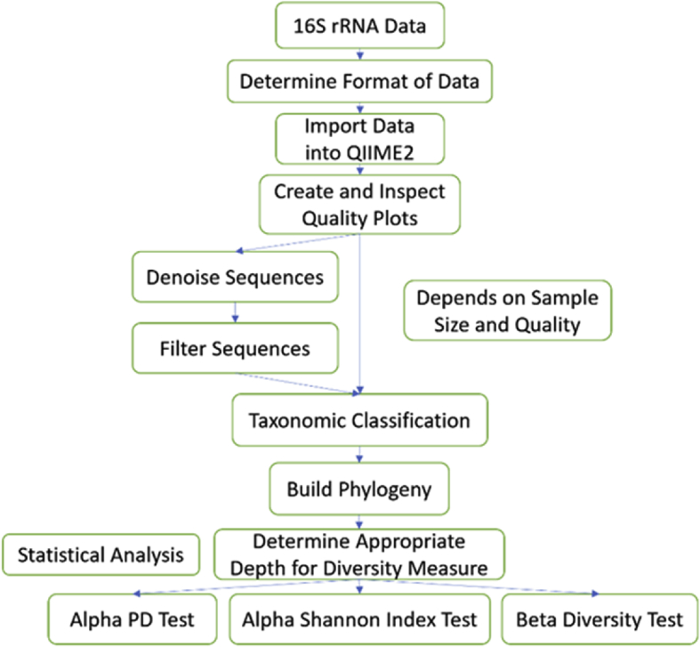
The microbiome data contain sequences, and transitioning from raw sequence data to useful results often requires significant work, but computational tools such as QIIME2 have made it much easier. QIIME2 is a microbiome analysis package that could translate raw sequence data into useful statistical results. It can be accessed at https://qiime2.org/.1 Researchers can simply follow the available pipeline that has been described in Hall and Beiko2 to generate their desired diversity tests and taxonomic profiles without knowing the statistical logic behind it. Even though the Hall and Beiko article is a perfect guideline for 16S rRNA data analysis, it is not a completely suitable for all datasets and, in fact, proper adjustments must be made. The Hall and Beiko robust dataset will be used here as a contrast to two pre-clinical datasets in the next section. Pre-clinical data have issues such as low-quality scores and small sample size. Those problems impact the use of truncation, and later the choice of sequence depth. A flowchart (Fig. 1) is provided as a guideline for 16S rRNA data analysis using QIIME2. Note that additional features could also be generated using QIIME2, such as taxonomic profiles bar plots, but those are not relevant to our purpose which is to identify potential issues when handling pre-clinical data.
Figure 1.
Flowchart for sequence data analysis using QIIME2.
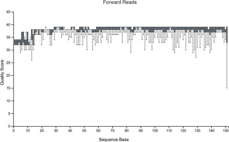
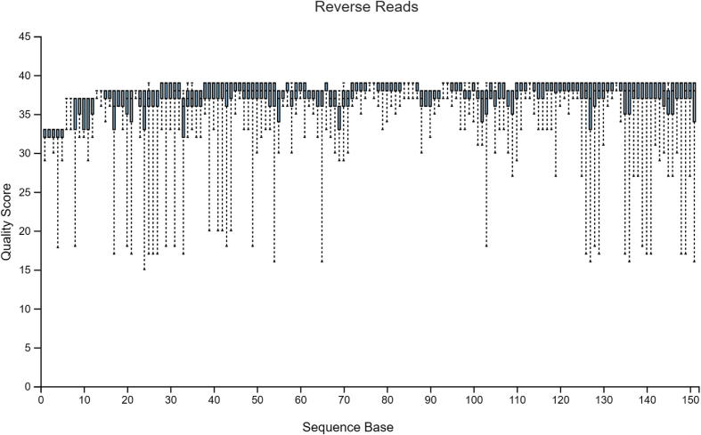
The sample data used in Hall and Beiko2 is a study on the gut microbiome of the bumblebee. There are 106 samples (paired-end) with a total frequency of more than one million data points. For pre-processing of raw sequencing reads prior to the subsequent analysis, it is necessary and important to perform a quality check. The quality plots can be found in Figure 2, Figure 3. Trimming was performed at position 19 in forward reads and position 20 in reverse reads. Based on quality plots, truncation was conducted at position 150 in forward reads and at position 140 in reverse reads. Samples with fewer than 5000 sequences were removed. A filtered table with sequence count can be found in Table 1. Since we are only using the result for visualized comparison, most of the table will be omitted. After filtering, the lowest sample has a total sequence of 42,162. The overall quality and sequence count are very good, and the result should be accurate. In the next section, we will show that pre-clinical data have relatively poorer conditions, and thus, might present a problem in terms of data analysis. Our sample data and code can be found at http://louisville.edu/medicine/research/cancer/cores-and-facilities-1/biodata.
Figure 2.
Quality plot for forward reads.
Figure 3.
Quality plot for reverse reads.
Table 1.
Filtered data with sequence count (partial).
| Sample ID | Sequence Count |
|---|---|
| SRR3202941 | 116,837 |
| SRR3202937 | 116,747 |
| SRR3202980 | 115,380 |
| SRR3202963 | 114,591 |
| SRR3202985 | 113,766 |
| …… | |
| 95 Omitted | |
| SRR3202967 | 50,081 |
| SRR3202968 | 49,572 |
| SRR3203000 | 47,816 |
| SRR3202970 | 46,850 |
| SRR3203003 | 42,162 |
First pre-clinical data application: Gingival microbiome study in knockout and wild-type mice
Sequence data
The 16S rRNA data in this application were obtained from the gingival surfaces of mice in a pre-clinical setting. The goal was to test whether there is any difference between knockout group and wild-type group in terms of gingival microbiome. There was a total of 10 samples (pair-end) distributed in two groups, with 5 samples in group 1 and 5 samples in group 2. The highest sequence count in a sample was 1,572, and the lowest sequence count in a sample was 87. Group significance tests were used for the analysis.
Methods
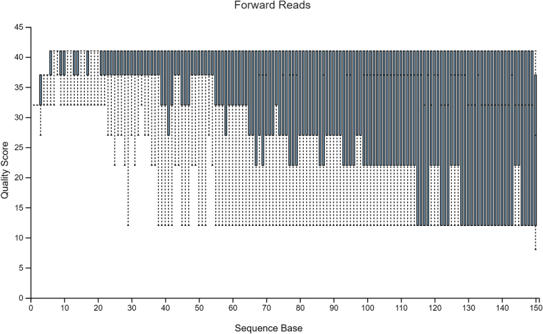
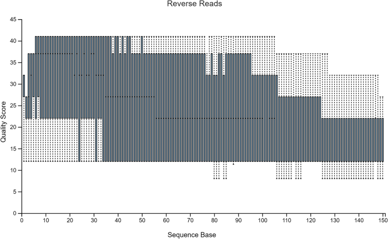
After importing the data into QIIME2, quality plots were produced and visualized (Fig. 4 and 5). In Fig. 4, the quality scores for forward reads began to drop more frequently starting at position 77 and became worse at position 115. In Fig. 5, the overall quality score looked consistent, but not optimal. Based on the general rule, truncation is needed when there is a big variance change in quality score, if the median quality score is below 20, or if the lowest quality score is below 5. In this case, the median quality score dropped below 20 at position 105. If one truncates too many sequences, there may not be sufficient samples left, given such a small sample size to start with. In addition, the position of truncation might also impact the outcome of the final test. To make a comparison, two sets of denoise procedures were conducted. In the first set, truncation was performed at position 149 for forward reads and position 125 for reverse reads, and trimming was conducted at position 17 for forward reads and position 19 for reverse reads. In the second set, truncation was performed at position 114 for forward reads and position 105 for reverse reads, and trimming was conducted at position 17 for forward reads and position 19 for reverse reads. Summary tables for both sets can be found in Table 2, Table 3, respectively.
Figure 4.
Quality plot for Forward Reads for Pre-clinical data.
Figure 5.
Quality plot for Reverse Reads for Pre-clinical data.
Table 2.
Summary Table with sequence count for first set.
| Sample ID | Group | Sequence Count |
|---|---|---|
| Sample 4 | 1 | 218 |
| Sample 2 | 1 | 180 |
| Sample 1 | 1 | 154 |
| Sample 5 | 1 | 104 |
| Sample 3 | 1 | 95 |
| Sample 10 | 2 | 79 |
| Sample 7 | 2 | 54 |
| Sample 9 | 2 | 0 |
| Sample 8 | 2 | 0 |
| Sample 6 | 2 | 0 |
Table 3.
Summary Table with sequence count for second set.
| Sample ID | Group | Sequence Count |
|---|---|---|
| Sample 4 | 1 | 259 |
| Sample 2 | 1 | 246 |
| Sample 1 | 1 | 208 |
| Sample 3 | 1 | 113 |
| Sample 5 | 1 | 99 |
| Sample 10 | 2 | 69 |
| Sample 7 | 2 | 65 |
| Sample 9 | 2 | 0 |
| Sample 8 | 2 | 0 |
| Sample 6 | 2 | 0 |
Depending on the experiment, filtering is needed to eliminate samples that have fewer sequence counts. In both sets of procedures, filtering was performed to remove samples that had no sequence count. Most researchers’ ultimate goals are significance tests to show if groups were different. A depth of 50 was picked. In this case, all remaining samples would be used for significance tests. Comparison of p-values can be found in Table 4.
Table 4.
Comparison of test statistics and p-value between two truncation locations.
| Depth at 50 |
||||
|---|---|---|---|---|
| First Set |
Second Set |
|||
| Test Statistics | p-value | Test Statistics | p-value | |
| Alpha Shannon | 3.818 | 0.051 | 3.335 | 0.068 |
| Beta Diversity | 1.131 | 0.539 | 1.072 | 0.524 |
Results
Different locations of truncation will result different sequence counts for each sample even though the number are at a margin in this specific data (Table 2, Table 3). After filtering, those samples with 0 sequence counts were removed. There remained 5 samples from group 1 and 2 samples from group 2 in both procedures.
There was some variation among p-values, especially for the alpha Shannon diversity test. The first set had a p-value just barely above 0.05, and the second set had a p-value at 0.068. A p-value of 0.051 can be interpreted differently, depending on the situation. For example, it might be clinically significant but statistically nonsignificant. These tests might produce opposite conclusions if the choice of truncation is not appropriate or justified. Thus, it is something that researchers should pay attention to.
Second Pre-clinical data application: Gut microbiome study in copper deficiency and high fructose diet fed mice
Sequence data
The 16S rRNA data in the second application was generated from rats in a pre-clinical setting as discussed in Song et al.3 The microbiome study was designated to test whether the combination of dietary marginal copper deficiency and high fructose diet (copper-fructose interactions) alters the gut microbiome, leading to gut microbiota dysbiosis, subsequently contributing to the development of metabolic diseases. There was a total of 10 samples (pair-end) distributed in two groups, with 5 samples in group 1 and 5 samples in group 2. The highest sequence count in a sample was around 89,400, and the lowest sequence count in a sample was around 26,100. Group significance tests were used for the analysis.
Methods
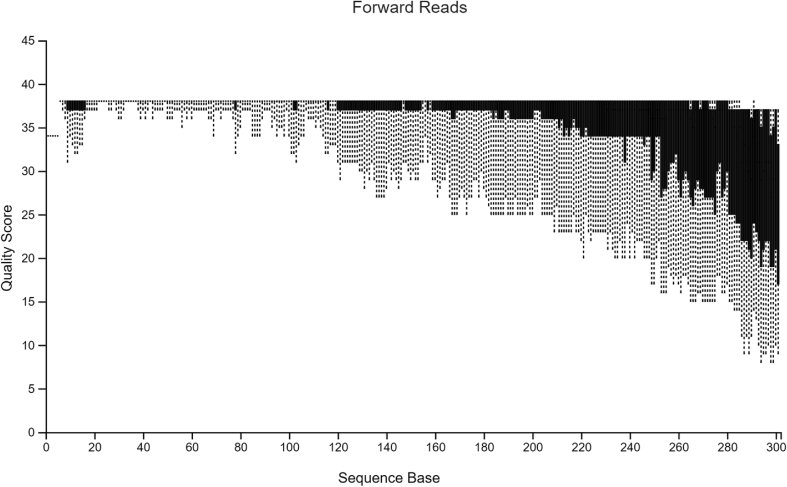
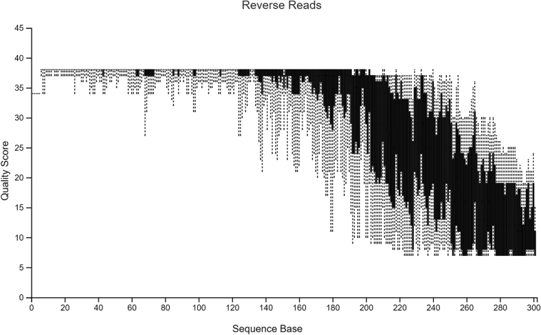
After importing the data into QIIME2, quality plots were produced and visualized (Fig. 6 and 7). In this dataset, truncation was performed at position 275 for forward reads and position 227 for reverse reads. Trimming was performed at position 50 for forward reads and position 55 for reverse reads. The summary table can be found in Table 5. We produced two depth options to see how it would impact the p-values that are most important to investigators. In the first option, depth was set at 20,000 since there is a relatively larger drop of sequence counts from Sample CM-01-Rat-CuA-2 to Sample CM-21-Rat-CuMF-25. Therefore, samples with sequence counts higher than 20,000 would be used for significance tests. In the second option, the goal was to save more samples. A depth of 10,000 was picked. In this case, all samples would be used for significance tests. Comparison of p-values can be found in Table 6.
Figure 6.
Quality plot for Forward Reads for the Second Pre-clinical data.
Figure 7.
Quality plot for Reverse Reads for the Second Pre-clinical data.
Table 5.
Summary Table with sequence count for the second dataset.
| Sample ID | Group | Sequence Count |
|---|---|---|
| CM-05-Rat-CuA-7 | 1 | 59,180 |
| CM-22-Rat-CuMF-26 | 2 | 56,085 |
| CM-03-Rat-CuA-4 | 1 | 51,217 |
| CM-04-Rat-CuA-5 | 1 | 50,307 |
| CM-02-Rat-CuA-3 | 1 | 47,106 |
| CM-23-Rat-CuMF-27 | 2 | 42,155 |
| CM-20-Rat-CuMF-24 | 2 | 36,280 |
| CM-01-Rat-CuA-2 | 1 | 34,013 |
| CM-21-Rat-CuMF-25 | 2 | 17,018 |
| CM-24-Rat-CuMF-28 | 2 | 16,541 |
Table 6.
Comparison of test statistics and P-value between two sampling depth.
| Depth at 10,000 |
Depth at 20,000 |
|||
|---|---|---|---|---|
| Test Statistics | P-Value | Test Statistics | P-Value | |
| Alpha Shannon | 0.011 | 0.917 | 0.199 | 0.655 |
| Beta Diversity | 1.526 | 0.065 | 1.560 | 0.102 |
Results
When depth was picked at 10,000, there were 5 samples from group 1 and 3 samples from group 2. Even though there were no significant differences between groups, p-values vary a lot in the Beta diversity test. It is also worth mentioning that the test statistics, or called H-Index in this case, are different in Alpha Shannon which produce a different diversity interpretation. At depth of 10,000, Beta diversity test has a P-value at 0.065 which can also be interpreted differently. While at depth of 20,000, it is certain that there is no significant difference in terms of beta diversity (P = 0.102). Different choice of depth may lead to opposite conclusions. Again, it depends on the experiment, but it is something that researchers should pay attention to.
Additional issues
We have seen some potential issues in pre-clinical data using QIIME2 with small sample size and low-quality score. There are some additional problems that are worth mentioning. Depending on the experiment and type of data, missing values should be considered. Moreover, normalization also must be considered, as suggested in Srivastava et al.4
Taxa count data are often over-dispersed in microbiome studies.5 The issue must be addressed before the analysis stream starts. Currently, there is a plugin available called corncob which was developed based on the R to be used in QIIME2. Note that the negative binomial is recommended when handling over-dispersed data as it outperforms the Poisson model.6
Importantly, when there are more groups and researchers wish to see the impact of interactions among those groups, QIIME2 does not have the ability to compute Two-Way ANOVA.
Statistical methods in microbiome study
Many classic statistical testing methods are available to analyze microbiome data. Detailed methods explanations including formulas can be found in: Statistical Analysis of Microbiome Data with R.7 It is very important for investigators doing the microbiome analysis to know the detailed calculations behind those codes. Hypothesis testing can be conducted by comparing alpha and beta diversity indices in microbial taxa. We can perform a t-test, ANOVA or non-parametric tests, depending on whether the data are normally or non-normally distributed. Typically, ANOVA works well when the data are normally distributed, but since most microbiome data are not normally distributed, the use of ANOVA is mostly limited to alpha diversity.
Two-sample t-test and the non-parametric Wilcoxon rank sum test are widely used in microbiome studies for comparing continuous variables, such as alpha diversity or population abundance, between two groups. The standard t-test is used to compare the relative abundances of different phyla and genera between any two groups. The Wilcoxon rank sum test is used to compare alpha diversity and Shannon diversity between two different bacterial taxonomic compositions.7 The Kruskal–Wallis test can also be used for non-normally distributed data. It is a non-parametric method for testing whether samples originated from the same distribution.8 The null hypothesis of the Kruskal–Wallis test is that the mean ranks of the groups are the same.
Analyses of community diversities are widely used in community microbiome studies, in which diversity translates to richness, the number of types and various diversity indices. Most diversity methods assume that data are the counts of individuals. The alpha diversity, beta diversity and gamma diversity have become central to community ecology. However, alpha diversity and beta diversity are the most commonly used in microbiome study. In microbiome study, alpha diversity is referred to as diversity within a single sample or within a community while beta diversity evaluates differences between two or more local assemblages or between local and regional assemblages.
Sample size calculation
As previously mentioned, the negative binomial distribution is a good choice for modeling when data are over-dispersed. Li et al.9 proposed several methods for calculating sample size in microbiome data. Detailed explanations and formulas can be found in that paper. On the other hand, Jung10 presented a sample size calculation method for a specified number of true rejections while controlling the false discovery rate at a desired level with a closed-form formula if the projected effect sizes are equal among differentially expressing genes; otherwise, a numerical method is required to solve an equation. In addition, rank-based procedures can also be used, in which case α can be adjusted using α divided by the number of groups. To demonstrate, we considered a hypothetical example. Suppose there are two type of samples (cases and controls) and potential number of types of bacteria are 120, of which about 30% are potential candidates to differ between cases and controls. Of the 30%, our focus is to identity at least 6 (5% of all 120). In this example, the adjusted alpha will be 0.0038, 0.0079 and 0.0126 at FDR values of 5%, 10% and 15%, respectively.10 We assume log transformed concentrations to be normally distributed. To detect the log concentration of at least 1.5 SD (standard deviation units) at power of 80% for one-sided hypothesis, we need 13, 11 and 10 samples of each type. If a two-sided hypothesis is used, the corresponding sample sizes will be 15, 13 and 12 (Table 7). If we consider a hypothesis generating pre-clinical study that does not adjust alpha, we will be able to detect reasonably small effect sizes (1.0 SD) with 12 animals in each group. If attrition is expected, these samples sizes must be increased to address the attrition.
Table 7.
Sample size required at power of 80% at different FDR level.
| FDR | Adjusted α | Sample Size Required |
|
|---|---|---|---|
| One-Sided | Two-Sided | ||
| 5% | 0.0038 | 13 | 15 |
| 10% | 0.0079 | 11 | 13 |
| 15% | 0.0126 | 10 | 12 |
Discussion
Different truncation locations can produce opposite result, as our first data application showed. Moreover, the choice of sampling depth can also create problems similar to the beta diversity we have in our second data application. In addition, the small sample size in our data has produced a barely acceptable result. The result would be much more supportive of the hypothesis if the minimum sample size for both groups were at least 12.
Problems such as small sample size and low-quality score are associated with pre-clinical data and often create problems for researchers. As shown above, appropriate actions must be taken in order to produce a meaningful and accurate result. Additionally, the assumption of normality often does not hold for microbiome data, and therefore, the data require further handling before analysis. In preclinical studies, based on our experience and sample size calculation it is recommended to use 12 evaluable samples in each setting. The calculation of sample size is important, as minimum size is required to reach the desired power.
Future research could focus on the development of additional features in QIIME2 such as Two-Way ANOVA. In addition, there are other ways to determine trimming and truncation. For example, some investigators would filter out the reads based on quality scores. This can be done in QIIME2. However, cutting out low quality score reads would dramatically shrink the data especially in a pre-clinical setting data that already does not have good quality scores in general. Future research could make a comparison between different methods of denoise when relatively better data are available.
Even though QIIME2 is a powerful tool in terms of sequence data analysis, the ability to adjust for certain conditions is limited. R has become a good statistical tool for 16S rRNA data analysis, as it is more flexible in calculations. Callahan et al.11 developed a full workflow for 16S rRNA data analysis using R, and it appears to be very useful.
Conflict of Interests
The authors declare no conflict of interests.
Acknowledgements
S. N. Rai was partly supported with Wendell Cherry Chair in Clinical Trial Research Fund and NIH grants 5P20GM113226 (CJM), 1P42ES023716 (PI: Sanjay Srivastava) and 1P20GM125504 (PI: Richard Lamont).
C. Qian was supported by the National Institutes of Health grant 5P50AA024337 (CJM) and the University of Louisville Fellowship.
Footnotes
Peer review under responsibility of Chongqing Medical University.
References
- 1.Bolyen E., Rideout J., Dillon M. Reproducible, interactive, scalable and extensible microbiome data science using QIIME 2. Nat Biotechnol. 2019;37:852–857. doi: 10.1038/s41587-019-0209-9. [DOI] [PMC free article] [PubMed] [Google Scholar]
- 2.Hall M., Beiko R.G. 16S rRNA gene analysis with QIIME2. Methods in Molecular Biology. 2018;1849:113–129. doi: 10.1007/978-1-4939-8728-3_8. [DOI] [PubMed] [Google Scholar]
- 3.Song M., Li X., Zhang X. Dietary copper-fructose interactions alter gut microbial activity in male rats. Am J Physiol Gastrointest Liver Physiol. 2018;314(1):G119–G130. doi: 10.1152/ajpgi.00378.2016. [DOI] [PMC free article] [PubMed] [Google Scholar]
- 4.Srivastava S., Merchant M., Rai A., Rai S.N. Standardizing proteomics workflow for liquid chromatography-mass spectrometry: technical and statistical considerations. J Proteom Bioinform. 2019;12(3):48–55. doi: 10.35248/0974-276x.19.12.496. [DOI] [PMC free article] [PubMed] [Google Scholar]
- 5.Xia Y., Sun J. Hypothesis testing and statistical analysis of microbiome. Genes Dis. 2017;4(3):138–148. doi: 10.1016/j.gendis.2017.06.001. [DOI] [PMC free article] [PubMed] [Google Scholar]
- 6.Xia Y., Morrison-Beedy D., Ma J., Feng C., Cross W., Tu X. Modeling Count Outcomes from HIV Risk Reduction Interventions: A Comparison of Competing Statistical Models for Count Responses. AIDS Res Treat. 2012;2012 doi: 10.1155/2012/593569. [DOI] [PMC free article] [PubMed] [Google Scholar]
- 7.Xia Y., Sun J., Chen D.G. Springer Nature Singapore Pte Ltd; 2018. Statistical Analysis of Microbiome Data with R. [Google Scholar]
- 8.Kruskal W.H., Wallis W.A. Use of ranks in one-criterion variance analysis. J Am Stat Assoc. 1952;47(260):583–621. [Google Scholar]
- 9.Li X., Wu D., Cooper N., Rai S.N. Sample size calculations for the differential expression analysis of RNA-seq data using a negative binomial regression model. Stat Appl Genet Mol Biol. 2019;18(1) doi: 10.1515/sagmb-2018-0021. [DOI] [PubMed] [Google Scholar]
- 10.Jung S.H. Sample size for FDR-control in microarray data analysis. Bioinformatics. 2005;21(14):3097–3104. doi: 10.1093/bioinformatics/bti456. [DOI] [PubMed] [Google Scholar]
- 11.Callahan B.J., Sankaran K., Fukuyama J.A., McMurdie P.J., Holmes S.P. Bioconductor Workflow for Microbiome Data Analysis: From Raw Reads to Community Analyses. F1000Res. 2016;5 doi: 10.12688/f1000research.8986.1. [DOI] [PMC free article] [PubMed] [Google Scholar]


