Fundamentals of integrated ferrohydrodynamic cell separation in circulating tumor cells isolation

Abstract

Methods to separate circulating tumor cells (CTCs) from blood samples were intensively researched in order to understand metastatic process and develop corresponding clinical assays. However current methods faced challenges that stemmed from CTCs’ heterogeneity in their biological markers and physical morphologies. To this end, we developed integrated ferrohydrodynamic cell separation (iFCS), a scheme that separated CTCs independent of their surface antigen expression and physical characteristics. iFCS integrated both diamagnetophoresis of CTCs and magnetophoresis of blood cells together via a magnetic liquid medium, ferrofluid, whose magnetization could be tuned by adjusting its magnetic volume concentration. In this paper, we presented the fundamental theory of iFCS and its specific application in CTC separation. Governing equations of iFCS were developed to guide its optimization process. Three critical parameters that affected iFCS’s cell separation performance were determined and validated theoretically and experimentally. These parameters included the sample flow rate, the volumetric concentration of magnetic materials in the ferrofluid, and the gradient of the magnetic flux density. We determined these optimized parameters in an iFCS device that led to a high recovery CTC separation in both spiked and clinical samples.

Graphical Abstract

We present the fundamental theory and experimental validations of an integrated ferrohydrodynamic cell separation (iFCS) method that can isolate circulating tumor cells with high recovery rate.

Introduction

Separation of circulating tumor cells (CTCs) from cancer patients’ blood samples had significant impacts on understanding the metastatic process and its diagnosis, prognosis, and treatment choices.^1–6 Individual and clustered CTCs were known to initiate metastasis that was responsible for over 90% of cancer-related death.^7–9 Clinical trials have shown that elevated levels of CTCs in cancer patients were associated with poor prognosis in metastatic and localized carcinomas.^10–12 As a result, CTC separation technologies have been intensively researched for the past decade with the hope that it would be routinely integrated into clinical assays.^{13, 14} However, the development of CTC separation faced challenges as CTCs were increasingly found to be not only a rare but also a heterogeneous cellular population of different phenotypic subtypes.^{1, 4, 8, 15–17} For instance, a fraction of epithelial tumor cells could transition into stem-like mesenchymal cells through epithelial to mesenchymal transition (EMT).^{7, 8, 18} This subpopulation of EMT CTCs were found to be highly migratory, invasive and have the potential to initiate a new tumor site.^{7, 8, 18} Given the phenotypic heterogeneity presented in patient-derived CTCs, and its extreme rarity in blood circulation, separation methods relying on specific biomarkers or physical features of these cells often leaded to incomplete recovery of these cells. As a result, new methods are urgently needed to allow for a comprehensive recovery of CTCs independent of their surface antigens and physical characteristics.¹³

Existing microfluidic CTC separation methods faced the same challenges in recovering CTCs because they either relied on the use of specific markers on tumor cells’ surface or physical features of tumor cells such as their elasticity or diameter.^{13, 14} The reliance of these markers or features were problematic in that CTCs were both biologically and physically heterogeneous.^{1, 4, 8, 15–17} Separation methods relying on tumor cells’ biomarkers such as epithelial cell adhesion molecule (EpCAM) missed CTCs undergoing EMT with their levels of EpCAM downregulated.¹⁹ On the other hand, separation methods relying on physical features of tumor cells operated on either the elasticity difference or a presumed size difference between blood and tumor cells.^{13, 14, 20, 21} For size difference based separation, CTCs in blood circulation were found to be polydispersed in their physical diameters. Clinically isolated CTCs were reported to have a diameter range of ~4 – 30 μm, which overlapped significantly with the diameters of white blood cells (WBCs), the main contaminant in CTC separation.^{22, 23} As a result, these methods either had to sacrifice CTC recovery in order to reduce WBC contamination by choosing a relatively larger size threshold, or sacrifice purity of CTCs in order to increase the recovery by choosing a smaller size threshold.^{13, 24} In either case, the inherent bias in both biomarker-dependent and size-dependent methods, and the recognition that CTCs were extremely rare and highly heterogeneous, highlight the need to develop new methods that can enrich CTCs regardless of their surface antigen and physical sizes.

To address the issues that faced existing CTC separation methods, we developed and studied a new CTC separation scheme, namely integrated ferrohydrodynamic cell separation (iFCS) method that allowed for the separation of CTCs independent of their surface antigen expression and physical features. The working principle of iFCS is illustrated in Figure 1. We integrated the principles of both “diamagnetophoresis” and “magnetophoresis” in iFCS for the simultaneous isolation of CTCs and depletion of white blood cells (WBCs). In this method, WBCs were rendered magnetic by magnetic beads with a combination of specific leukocyte biomarkers, while CTCs remained label-free. Without cell focusing, WBC-bead complex and CTCs continuously flowed through an iFCS device filled with a magnetic liquid medium called ferrofluids, whose magnetization were tuned and optimized so that unlabeled CTCs were expelled from the magnets due to “diamagnetophoresis” depending on their physical sizes, while WBC-bead complexes were attracted to the magnets through “magnetophoresis” depending on their levels of magnetization. As a result, CTCs regardless of their biomarker expressions and size profiles were continuously separated from WBCs in iFCS without cell focusing. To the best of our knowledge, iFCS was the first method that magnetically separated cells based on both their magnetic properties and physical sizes, which differed significantly from either diamagnetophoresis or magnetophoresis alone (Figures 1A and 1B). In diamagnetophoretic methods,^25–29 manipulation specificity of cells predominately focused cell size, and the difference in magnetic properties, such magnetization between cells were not investigated for the purpose of cell separation. On the other hand, manipulation specificity of magnetophoresis relied on only the magnetic properties of cells, which typically led to the binary separation of magnetic objects from diamagnetic ones, lacking the ability to separate cells based on the level of their magnetization.^30–32 In contrast, iFCS made use of both cellular magnetic property and physical size together to separate cells from each other. Ferrofluids, the magnetic liquid medium used in iFCS, provided a tunable liquid environment so that diamagnetophoresis and magnetophoresis co-existed and took effect on cells simultaneously. Unlabeled and diamagnetic CTCs were directed away from the WBCs that are magnetically labeled and more magnetic than the ferrofluid, leading to a complete recovery of CTCs. iFCS was shown recently to isolate CTCs from cancer patients’ blood in a biocompatible manner and achieved high recovery and low WBC contamination.³³ In this paper, we presented the fundamental theory of iFCS, its design and optimization process in a device with simple geometry and configuration, three important parameters that affected the performance of iFCS, and the validation of the device using microbeads, spiked samples as well as clinical samples.

Figure 1.

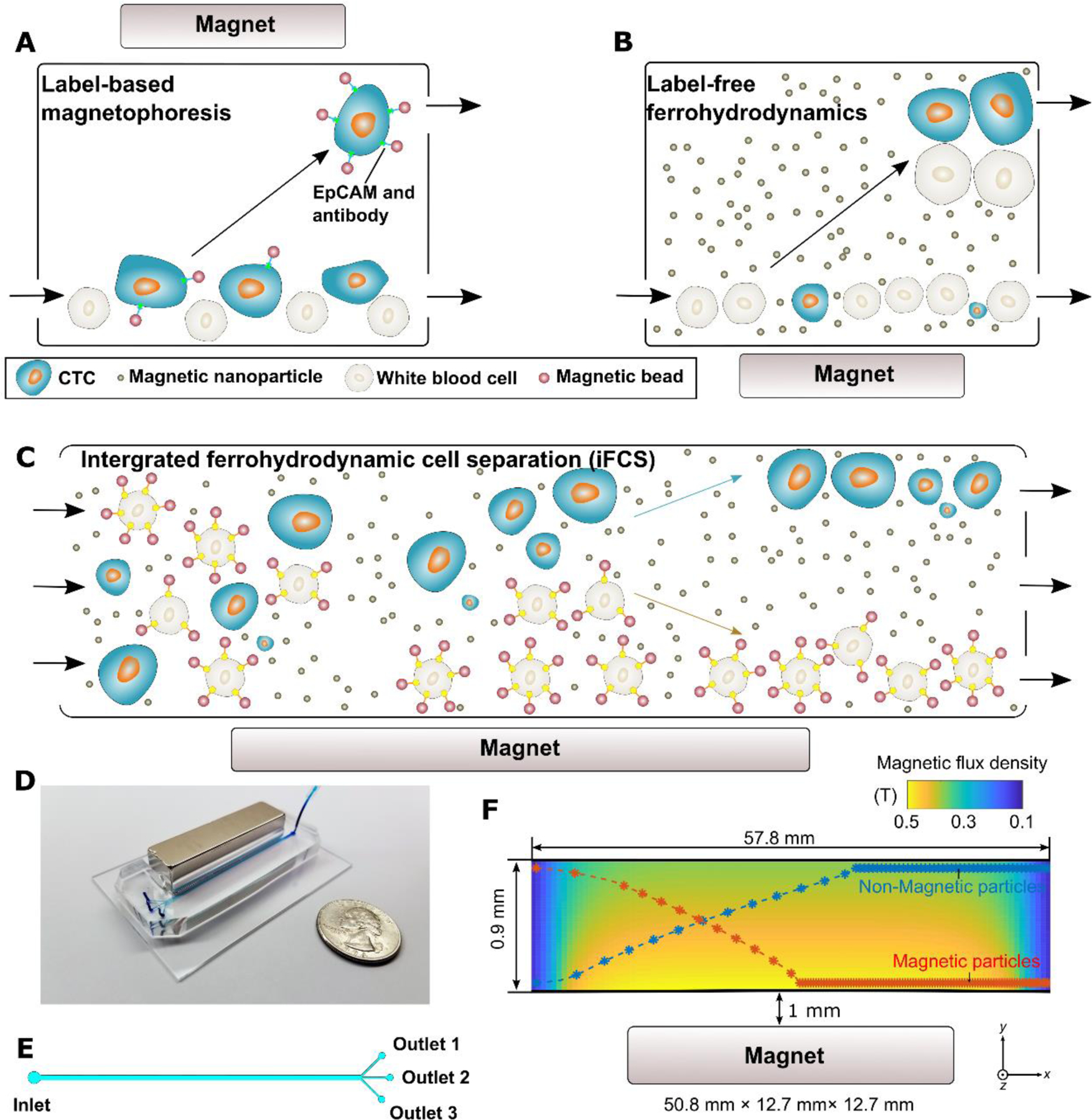
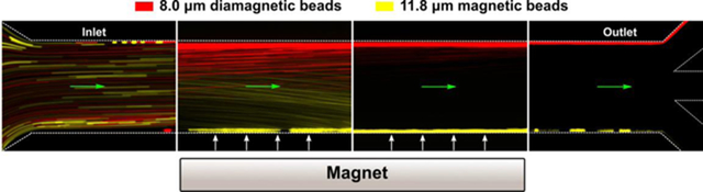
Overview of integrated ferrohydrodynamic cell separation (iFCS) and its prototype. (A) Schematic illustration of a traditional label-based magnetophoresis for CTC separation, in which CTCs were labeled via specific biomarkers such as epithelial cell adhesion molecule (EpCAM) through functionalized magnetic particles to be separated by magnetic force towards magnetic field maxima in a continuous-flow manner. (B) Schematic illustration of a label-free ferrohydrodynamic cell separation of CTCs. CTCs with increased physical sizes in ferrofluid experienced increased magnetic buoyance force via diamagnetophoresis and were pushed towards the magnetic field minimum. (C) Schematic illustration of an integrated ferrohydrodynamic cell separation (iFCS) scheme for CTC isolation. Unlabeled CTCs of different sizes and magnetically labeled WBCs were pushed towards opposite directions via different mechanisms (diamagnetophoresis for CTCs and magnetophoresis for WBCs), resulting in a spatial separation at the end of the device. (D) A prototype iFCS device. (E) Top view of the iFCS microchannel with labels of the inlet and outlets. (F) Simulated magnetic flux density distribution and trajectories of 11.8 μm magnetic beads and 15 μm diamagnetic beads in the microchannel (L×W×H, 57.8 mm×0.9 mm×0.15 mm) with a neodymium permanent magnet (L×W×H, 50.8 mm×12.7 mm×12.7 mm). The dimensions of the microchannel and the magnet were not drawn to scale. Particles were simulated using 0.05% (v/v) ferrofluid and a flow rate of 200 μL/min.

Results and discussion

Governing equations of iFCS

(1). Analysis of magnetic force on a magnetizable body in a magnetizable fluid (ferrofluids)

We first estimated the dominant forces on cells in iFCS. The forces included magnetic force and hydrodynamic viscous drag force. Other forces were negligible comparing to these two.^{34, 35} Microscopically, a magnetizable cell experienced both “diamagnetophoresis” from the magnetic nanoparticles in the ferrofluid colliding with its cellular surface, and “magnetophoresis” from its attached magnetic beads. We have obtained an expression of the force on the cell through the analysis of the magnetic stress tensor.³⁶ The stress tensor of a magnetizable fluid ${\overrightarrow{\overrightarrow{\text{T}}}}_{\text{m}}$ is given by the following expression

$${\overrightarrow{\overrightarrow{\text{T}}}}_{\text{m}}=-\left\{p(\rho ,T)+\underset{0}{\overset{H}{\int }}{\mu }_0{\left(\frac{\partial \left(\upsilon M\right)}{\partial \upsilon }\right)}_{H,T}dH+\frac{1}{2}{\mu }_0{H}^2\right\}\overrightarrow{\overrightarrow{\text{I}}}+\overrightarrow{\text{B}}\overrightarrow{\text{H}}$$ (1)

where $p(\rho ,T)$ is thermodynamic pressure that depends on the density of the fluid $\rho$, and the temperature T. H is the applied magnetic field strength, ${\mu }_0$ is the permeability of the free space, $\upsilon$ is the specific volume and $\upsilon ={\rho }^{-1}$, M is the magnetization. $\overrightarrow{\overrightarrow{\text{I}}}$ is the unit dyadic, $\overrightarrow{\text{B}}$ is the magnetic flux density vector, and $\overrightarrow{\text{H}}$ is the magnetic field strength vector. We also define a composite pressure term $p^{*}$ that is,

$$p^{*}=p(\rho ,T)+p_{\text{s}}+p_{\text{m}}$$ (2)

where $p_{\text{s}}$ is the magnetostrictive pressure which takes the following form

$$p_{\text{s}}={\mu }_0\underset{0}{\overset{H}{\int }}\upsilon {\left(\frac{\partial M}{\partial \upsilon }\right)}_{H,T}dH$$ (3)

and $p_{\text{m}}$ is the fluid-magnetic pressure which takes the following form

$$p_{\text{m}}={\mu }_0\underset{0}{\overset{H}{\int }}MdH={\mu }_0\overline{M}H$$ (4)

where $\overline{M}=\frac{1}{H}\underset{0}{\overset{H}{\int }}MdH$ is the field averaged magnetization.

We define ${\overrightarrow{\text{F}}}_{\text{m}}^{+}$ as the magnetic force exerted by the magnetizable fluid on just outside of a magnetizable body, which takes the following form

$${\overrightarrow{\text{F}}}_{\text{m}}^{+}=\nabla \cdot {\overrightarrow{\overrightarrow{\text{T}}}}_{\text{m}}=\underset{S}{\oint }\overrightarrow{\text{n}}\cdot {\overrightarrow{\overrightarrow{\text{T}}}}_{\text{m}}dS=\underset{S}{\oint }{\overrightarrow{\text{t}}}_{\text{n}}dS$$ (5)

where

$${\overrightarrow{\text{t}}}_{\text{n}}=\overrightarrow{\text{n}}\cdot {\overrightarrow{\overrightarrow{\text{T}}}}_{\text{m}}$$ (6)

where $\overrightarrow{\text{n}}$ is the unit vector normal to the surface of the magnetizable body.

From Eqs. (1), (2) and (6), we can get the following expression of the magnetic force

$${\overrightarrow{\text{F}}}_{\text{m}}^{+}=\underset{S+}{\oint }\left(-\left(p^{*}+\frac{1}{2}{\mu }_0{H}^2\right)\overrightarrow{\text{n}}+\overrightarrow{\text{H}}{B}_{\text{n}}\right)$$ (7)

From the ferrohydrodynamic Bernoulli equation,³⁶ we get

$$p^{*}+\rho gh-{\mu }_0\overline{M}H=p_0+\rho g{h}_0$$ (8)

From Eqs. (7) and (8), we get

$${\overrightarrow{\text{F}}}_{\text{m}}^{+}=\underset{S+}{\oint }\left(\left(-p_0-\rho g{h}_0+\rho gh-{\mu }_0\overline{M}H-\frac{1}{2}{\mu }_0{H}^2+H_{\text{n}}{B}_{\text{n}}\right)\overrightarrow{\text{n}}+H_{\text{t}}{B}_{\text{n}}\overrightarrow{\text{t}}\right)dS$$ (9)

where $\overrightarrow{\text{H}}=H_{\text{n}}\overrightarrow{\text{n}}+H_{\text{t}}\overrightarrow{\text{t}}$ is used, $\overrightarrow{\text{t}}$ is the unit vector tangential to the surface of the magnetizable body.

We apply the divergence theorem to the following term in Eq. (9), which results in

$$\underset{S+}{\oint }\left(-\left(p_0+\rho g{h}_0\right)\right)\overrightarrow{n}dS=\underset{V}{\int }-\left(\nabla \left(p_0+\rho g{h}_0\right)\right)dV=0$$ (10)

Therefore

$${\overrightarrow{\text{F}}}_{\text{m}}^{+}=\underset{S+}{\oint }\left(\left(-{\mu }_0\overline{M}H-\frac{1}{2}{\mu }_0{H}^2+H_{\text{n}}{B}_{\text{n}}\right)\overrightarrow{\text{n}}+H_{\text{t}}{B}_{\text{n}}\overrightarrow{\text{t}}\right)dS$$ (11)

In Eq. (11), we can rewrite the term ${\mu }_0\overline{M}H+\frac{1}{2}{\mu }_0{H}^2$ as the following term

$${\mu }_0\overline{M}H+\frac{1}{2}{\mu }_0{H}^2=\underset{0}{\overset{H}{\int }}{\mu }_0\left(M+H\right)dH=\underset{0}{\overset{H}{\int }}BdH$$ (12)

As a result, the magnetic force exerted by the magnetizable fluid on a magnetizable body has the following expression

$${\overrightarrow{\text{F}}}_{\text{m}}^{+}=\underset{S+}{\oint }\left(\left(H_{\text{n}}{B}_{\text{n}}-\underset{0}{\overset{H}{\int }}BdH\right)\overrightarrow{\text{n}}+H_{\text{t}}{B}_{\text{n}}\overrightarrow{\text{t}}\right)dS$$ (13)

Similarly, we can obtain the magnetic force exerted on just inside of a magnetizable body

$${\overrightarrow{\text{F}}}_{\text{m}}^{-}=\underset{S-}{\oint }\left(\left(H_{\text{n}}{B}_{\text{n}}-\underset{0}{\overset{H}{\int }}BdH\right)\overrightarrow{\text{n}}+H_{\text{t}}{B}_{\text{n}}\overrightarrow{\text{t}}\right)dS$$ (14)

The net force exerted by the magnetizable fluid on a magnetizable body ${\overrightarrow{\text{F}}}_{\text{m}}$, which is the difference between ${\overrightarrow{\text{F}}}_{\text{m}}^{+}$ and ${\overrightarrow{\text{F}}}_{\text{m}}^{-}$, takes the following form

$${\overrightarrow{\text{F}}}_{\text{m}}={\overrightarrow{\text{F}}}_{\text{m}}^{+}-{\overrightarrow{\text{F}}}_{\text{m}}^{-}=\left\{\underset{S+}{\oint }\left(H_{\text{n}}{B}_{\text{n}}-\underset{0}{\overset{H}{\int }}BdH\right)\overrightarrow{\text{n}}dS-\underset{S-}{\oint }\left(H_{\text{n}}{B}_{\text{n}}-\underset{0}{\overset{H}{\int }}BdH\right)\overrightarrow{\text{n}}dS\right\}+\left\{\underset{S+}{\oint }{H}_{\text{t}}{B}_{\text{n}}\overrightarrow{\text{t}}dS-\underset{S-}{\oint }{H}_{\text{t}}{B}_{\text{n}}\overrightarrow{\text{t}}dS\right\}$$ (15)

Eq. (15) states that the expression of ${\overrightarrow{\text{F}}}_{\text{m}}$ can be calculated from the solutions of the magnetic fields alone. Because the tangential component of magnetic field strength $H_{\text{t}}$, and the normal component of magnetic flux density $B_{\text{n}}$ are continuous across the boundary of the magnetizable body, we get the following

$$H_{\text{t}}^{+}=H_{\text{t}}^{-},B_n^{+}=B_n^{-}$$ (16)

where the + sign indicates the location just outside the body and the − sign indicates the location just inside the body. As a result, we get

$${\left(H_{\text{t}}{B}_{\text{n}}\right)}^{+}={\left(H_{\text{t}}{B}_{\text{n}}\right)}^{-}$$ (17)

From Eqs. (15) and (17), we get

$${\overrightarrow{\text{F}}}_{\text{m}}=\left\{\underset{S+}{\oint }{H}_{\text{n}}{B}_{\text{n}}\overrightarrow{\text{n}}dS-\underset{S-}{\oint }{H}_{\text{n}}{B}_{\text{n}}\overrightarrow{\text{n}}dS\right\}-\left\{\underset{S+}{\oint }\left(\underset{0}{\overset{H}{\int }}BdH\right)\overrightarrow{\text{n}}dS-\underset{S-}{\oint }\left(\underset{0}{\overset{H}{\int }}BdH\right)\overrightarrow{\text{n}}dS\right\}$$ (18)

For convenience, we define the following

$$\left[H_{\text{n}}{B}_{\text{n}}\right]={\left(H_{\text{n}}{B}_{\text{n}}\right)}^{+}-{\left(H_{\text{n}}{B}_{\text{n}}\right)}^{-}$$ (19)

$$\left[\underset{0}{\overset{H}{\int }}BdH\right]=\underset{0}{\overset{H^{+}}{\int }}{B}^{+}d{H}^{+}-\underset{0}{\overset{H-}{\int }}{B}^{-}d{H}^{-}$$ (20)

As a result of Eqs. (19) and (20), Eq. (18) becomes

$${\overrightarrow{\text{F}}}_{\text{m}}=\underset{S}{\oint }\left[H_{\text{n}}{B}_{\text{n}}\right]\overrightarrow{\text{n}}dS-\underset{S}{\oint }\left[\underset{0}{\overset{H}{\int }}BdH\right]\overrightarrow{\text{n}}dS$$ (21)

Because the normal component of magnetic flux density $B_{\text{n}}$ is continuous across the boundary of the magnetizable body, we get

$${\overrightarrow{\text{F}}}_{\text{m}}=\underset{S}{\oint }{B}_{\text{n}}\left[H_{\text{n}}\right]\overrightarrow{\text{n}}dS-\underset{S}{\oint }\left[\underset{0}{\overset{H}{\int }}BdH\right]\overrightarrow{\text{n}}dS$$ (22)

We get the following expression for both $\left[H_{\text{n}}\right]$ and $\left[\underset{0}{\overset{H}{\int }}BdH\right]$

$$\left[H_{\text{n}}\right]=H_{\text{n}}^{+}-H_{\text{n}}^{-}=\left(\frac{B_{\text{n}}^{+}}{{\mu }_0}-M_{\text{n}}^{+}\right)-\left(\frac{B_{\text{n}}^{-}}{{\mu }_0}-M_{\text{n}}^{-}\right)=-\left(M_{\text{n}}^{+}-M_{\text{n}}^{-}\right)$$ (23)

$$\begin{gathered} \left[\underset{0}{\overset{H}{\int }}BdH\right]=\underset{0}{\overset{H^{+}}{\int }}{B}^{+}d{H}^{+}-\underset{0}{\overset{H^{-}}{\int }}{B}^{-}d{H}^{-}=\underset{0}{\overset{H^{+}}{\int }}{\mu }_0\left(M^{+}+H^{+}\right)d{H}^{+}-\underset{0}{\overset{H^{-}}{\int }}{\mu }_0\left(M^{-}+H^{-}\right)d{H}^{-} \\ ={\mu }_0\left(\underset{0}{\overset{H^{+}}{\int }}{M}^{+}d{H}^{+}-\underset{0}{\overset{H^{-}}{\int }}{M}^{-}d{H}^{-}\right)+\frac{1}{2}{\mu }_0\left(\frac{2B}{{\mu }_0}-M^{+}-M^{-}\right)\left(M^{-}-M^{+}\right) \end{gathered}$$ (24)

From Eqs. (22), (23) and (24), we get

$${\overrightarrow{\text{F}}}_{\text{m}}=\underset{S}{\oint }\left\{-B_{\text{n}}\left(M_{\text{n}}^{+}-M_{\text{n}}^{-}\right)+B\left(M^{+}-M^{-}\right)-\frac{1}{2}{\mu }_0\left({\left(M^{+}\right)}^2-{\left(M^{-}\right)}^2\right)-{\mu }_0\left(\underset{0}{\overset{H^{+}}{\int }}{M}^{+}d{H}^{+}-\underset{0}{\overset{H-}{\int }}{M}^{-}d{H}^{-}\right)\right\}\overrightarrow{\text{n}}dS$$ (25)

Because

$$\underset{S}{\oint }{B}_{\text{n}}\left(M_{\text{n}}^{+}-M_{\text{n}}^{-}\right)\overrightarrow{\text{n}}dS=\underset{S}{\oint }B\left(M^{+}-M^{-}\right)\overrightarrow{\text{n}}dS$$ (26)

We get

$${\overrightarrow{\text{F}}}_{\text{m}}=\underset{S}{\oint }\left\{-\frac{1}{2}{\mu }_0\left({\left(M^{+}\right)}^2-{\left(M^{-}\right)}^2\right)-{\mu }_0\left(\underset{0}{\overset{H^{+}}{\int }}{M}^{+}d{H}^{+}-\underset{0}{\overset{H-}{\int }}{M}^{-}d{H}^{-}\right)\right\}\overrightarrow{\text{n}}dS$$ (27)

Because $\overline{M}=\frac{1}{H}\underset{0}{\overset{H}{\int }}MdH$ is defined as the field averaged magnetization, we get

$${\overrightarrow{\text{F}}}_{\text{m}}=-\underset{S}{\oint }\left\{\frac{1}{2}{\mu }_0\left({\left(M^{+}\right)}^2-{\left(M^{-}\right)}^2\right)+{\mu }_0\left({\overline{M}}^{+}{H}^{+}-{\overline{M}}^{-}{H}^{-}\right)\right\}\overrightarrow{\text{n}}dS$$ (28)

By applying divergence theorem to Eq. (28), we get

$$\begin{gathered} {\overrightarrow{\text{F}}}_{\text{m}}=-\underset{S}{\oint }\left\{\frac{1}{2}{\mu }_0\left({\left(M^{+}\right)}^2-{\left(M^{-}\right)}^2\right)+{\mu }_0\left({\overline{M}}^{+}{H}^{+}-{\overline{M}}^{-}{H}^{-}\right)\right\}\overrightarrow{\text{n}}dS \\ =-\underset{V}{\int }\nabla \left(\frac{1}{2}{\mu }_0\left({\left(M^{+}\right)}^2-{\left(M^{-}\right)}^2\right)+{\mu }_0\left({\overline{M}}^{+}{H}^{+}-{\overline{M}}^{-}{H}^{-}\right)\right)dV \\ \approx -V\nabla \left(\frac{1}{2}{\mu }_0\left({\left(M^{+}\right)}^2-{\left(M^{-}\right)}^2\right)+{\mu }_0\left({\overline{M}}^{+}{H}^{+}-{\overline{M}}^{-}{H}^{-}\right)\right) \end{gathered}$$ (29)

where V is the volume of the magnetizable cell. In the case of an intensively applied magnetic field, we get

$$\frac{1}{2}{\mu }_0\left({\left(M^{+}\right)}^2-{\left(M^{-}\right)}^2\right)\ll {\mu }_0\left({\overline{M}}^{+}{H}^{+}-{\overline{M}}^{-}{H}^{-}\right)$$ (30)

Therefore

$${\overrightarrow{\text{F}}}_{\text{m}}=-V\nabla \left({\mu }_0\left({\overline{M}}^{+}{H}^{+}-{\overline{M}}^{-}{H}^{-}\right)\right)=-{\mu }_{0}V\left({\overline{M}}^{+}-{\overline{M}}^{-}\right)\nabla H$$ (31)

Consider the case where the ferrofluid is just outside the magnetizable body, we denote $M_{\mathit{\text{ferrofluid}}}$ to represent ${\overline{M}}^{+}$, and $M_{\mathit{\text{cell}}}$ to represent ${\overline{M}}^{-}$. The expression of the net magnetic force is then

$${\overrightarrow{\text{F}}}_{\text{m}}=-{\mu }_{0}V\left\{\left({\overrightarrow{\text{M}}}_{\text{ferrofluid}}-{\overrightarrow{\text{M}}}_{\text{cell}}\right)\cdot \nabla \right\}\overrightarrow{\text{H}}$$ (32)

(2). Analysis of hydrodynamic viscous drag force in ferrofluids

The magnetic force ${\overrightarrow{\text{F}}}_{\text{m}}$ acting on the cell is balanced by the hydrodynamic viscous drag force ${\overrightarrow{\text{F}}}_{\text{d}}$, when there is a relative motion between the cell and the fluid flow. Its expression is,

$${\overrightarrow{\mathbf{\text{F}}}}_{\text{d}}=-3\pi \eta D_p\left({\overrightarrow{\mathbf{\text{v}}}}_p-{\overrightarrow{\mathbf{\text{v}}}}_f\right)\lambda$$ (33)

Where $\eta$ is the ferrofluid viscosity, $D_p$ is the diameter of a spherical object, ${\overrightarrow{\mathbf{\text{v}}}}_p$ and ${\overrightarrow{\mathbf{\text{v}}}}_f$ are the velocity vectors of the ferrofluid and the object. $\lambda$ includes the parallel (${\lambda }_{\parallel }$) and perpendicular (${\lambda }_{\perp }$) components of the hydrodynamic drag force coefficient of a moving object after taking into account the influence from one nearby flat surface.^{37, 38} Its appearance indicates increased fluid viscosity as the object moves closer to the solid surface.

$${\lambda }_{\parallel }={\left[1-\frac{9}{16}\left(\frac{D_p}{D_p+2\Delta }\right)+\frac{1}{8}{\left(\frac{D_p}{D_p+2\Delta }\right)}^3-\frac{45}{256}{\left(\frac{D_p}{D_p+2\Delta }\right)}^4-\frac{1}{16}\left(\frac{D_p}{D_p+2\Delta }\right)\right]}^{-1}$$ (34)

$${\lambda }_{\perp }={\left[1-\frac{9}{8}\left(\frac{D_p}{D_p+2\Delta }\right)+\frac{1}{2}{\left(\frac{D_p}{D_p+2\Delta }\right)}^3\right]}^{-1}$$ (35)

where $\Delta$ is the shortest distance between the solid surface and the surface of the object. The balance of Eqs. (32) and (33) under laminar flow condition at low Reynold’s number was used to predict the trajectories of magnetizable cells, which in turn guided the optimization of iFCS devices in its application in CTC separation. Full set of equations in three-dimensional space are in the supplementary information.

Measurement and approximation of critical parameters in iFCS

Equations developed in the previous section indicated that the primary operating parameters that affected the CTC separation performance of the iFCS devices included sample processing throughput (sample flow rates), gradient of applied magnetic fields, volume fraction of magnetic materials in ferrofluids. Therefore it was critical to determine the magnetic field distribution and the ferrofluid concentration both experimentally and analytically so that both could be included in parametric studies to optimize iFCS. Here we discussed the approaches to determine and approximate magnetic fields, ferrofluid concentrations, and viscosity.

(1). Measurement and approximation of magnetizations of ferrofluids and magnetic beads

Theoretically, the magnetization of either a ferrofluid or micron-sized magnetic beads can be modeled through a Langevin function, assuming that the concentration of magnetic nanoparticles within a ferrofluid or micron-sized magnetic beads are small enough so that these nanoparticles are non-interacting. For a ferrofluid or micron-sized magnetic beads with a log-normal diameter distribution, we get their magnetization as^{39, 40}

$$M\left(\alpha \right)=M_s\underset{0}{\overset{\infty }{\int }}{n}_v\left(D_m\right)L\left(\alpha \right)d{D}_m$$ (36)

where $M_s$ is the saturation magnetization of the ferrofluid of the magnetic microbeads and $n_v\left(D_m\right)$ is the log-normal distribution of nanoparticle diameters which takes the following form

$$n_v\left(D_m\right)=\frac{1}{\sqrt{2\pi }{D}_m\text{ln}\sigma }\text{exp}\left\{\frac{-{\text{ln}}^2\left(D_m/D_{mv}\right)}{2{\text{ln}}^2\sigma }\right\}$$ (37)

where $D_m$ is the diameter of the magnetic nanoparticles, $D_{mv}$ is the volume-weighted median magnetic nanoparticle diameter, $\sigma$ is the geometric standard deviation of the magnetic nanoparticle diameter distribution. $L\left(\alpha \right)$ is the dimensionless Langevin function

$$L\left(\alpha \right)=\text{coth}\left(\alpha \right)-1/\alpha$$ (38)

where $\alpha$ is the Langevin parameter representing the ratio of magnetic to thermal energy

$$\alpha =\frac{{\mu }_0\pi M_d{D}_m^{3}H}{6k_{B}T}$$ (39)

where $M_d$ is the bulk magnetization of the magnetic materials, ${\mu }_0$ is the permeability of free space, H is the strength of the magnetic field, $k_B$ is the Boltzmann constant and T is the temperature. The relationship between bulk magnetization $M_d$ and saturation magnetization $M_s$ is

$$M_s=\varphi M_d$$ (40)

where $\varphi$ is the volume fraction of magnetic materials in the ferrofluid or magnetic microbeads.

Experimentally, the magnetization of either a ferrofluid or micron-sized magnetic particles can be measured at equilibrium via a vibrating sampling magnetometer (VSM). We can then fit the experimental equilibrium magnetization curve to the Eq. (36) to obtain magnetic properties including $D_m$, $D_{mv}$, $\alpha$, $\varphi$ and other relevant parameters. A maghemite based ferrofluid synthesized and used in this study was characterized by the VSM, whose data was fitted to the Langevin function in Figures 2A and 2B. Full measurement and fitting of VSM data on the ferrofluid and a commercial magnetic bead were in the supplementary information. These magnetic parameters of the ferrofluid and the magnetic beads were used in parametric studies for iFCS optimization.

Figure 2.

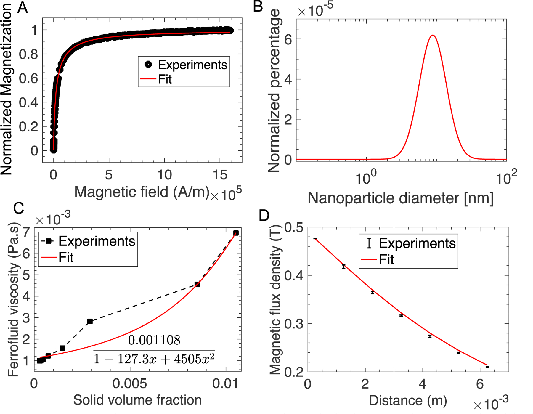
Experimental measurement and analytical approximation of critical operating parameters in iFCS. (A) Normalized experimental magnetization curve and fitted Langevin function of a maghemite ferrofluid used in this study. Fitted data at high field magnetization yielded a saturation magnetization $M_s$ of 1,085 A/m, which corresponded to a volume fraction $\varphi$ of 0.029 of magnetic materials in this ferrofluid. Goodness of fit (R²) was 0.999. Full measurement data were in the supplementary information. (B) Fitted data of the magnetization curve with a log-normal distribution of particle diameters yielded a volume-weighted median magnetic nanoparticle diameter $D_{mv}$ of 10.8 nm, and a geometric standard deviation of the magnetic nanoparticle diameter distribution $\text{ln}\sigma$ of 0.44. Temperature was 298 K, bulk magnetization of maghemite was 370,000 A/m, density of the ferrofluid was 1060.6 kg/m³, demagnetization factor due to the sample holder of the vibrating sampling magneto-meter was 0.211. (C) Experimentally measured ferrofluid viscosity and its fitted curve under no external magnetic field. The ferrofluid was a suspension of maghemite nanoparticles in a mixture of water and HBSS buffer with Atlox 4913 (Croda, Inc., Edison, NJ) graft copolymer as surfactants. Goodness of fit (R²) was 0.979. (D) Comparison of the measured magnetic flux density (error bar was the standard deviation of 3 measurements) to the analytical expressions in Eqs. (41–43). The x-axis label is the distance between the active area of the sensor and the magnet surface. The dimensions of the neodymium magnet were (L×W×H, 50.8 mm×12.7 mm×12.7 mm). The remnant magnetization from this fit was determined to be 1,055,693 A/m (residual magnetic flux density 1.33 T). Goodness of fit (normalized mean square error) was 0.997 (1 was perfect fit).

(2). Measurement and approximation of magnetic fields from permanent magnet(s)

We can get an analytical expression of the distribution of the magnetic field strength $\overrightarrow{\text{H}}$ of a rectangular permanent magnet.⁴¹ Assuming that the magnetic polarization of the magnet is in the +y direction (see Figure 1F for coordinates), the x and z components of the magnetic field strength, $H_x$ and $H_z$, have similar expressions as

$$H_x=\frac{M_r}{4\pi }\sum _{k=1}^2\sum _{m=1}^2{\left(-1\right)}^{k+m}\times \text{ln}\left\{\frac{\left(z-z_1\right)+{\left[{\left(x-x_m\right)}^2+{\left(z-z_1\right)}^2+{\left(y-y_k\right)}^2\right]}^{1/2}}{\left(z-z_2\right)+{\left[{\left(x-x_m\right)}^2+{\left(z-z_2\right)}^2+{\left(y-y_k\right)}^2\right]}^{1/2}}\right\}$$ (41)

$$H_z=\frac{M_r}{4\pi }\sum _{k=1}^2\sum _{m=1}^2{\left(-1\right)}^{k+m}\times \text{ln}\left\{\frac{\left(x-x_1\right)+{\left[{\left(x-x_1\right)}^2+{\left(z-z_m\right)}^2+{\left(y-y_k\right)}^2\right]}^{1/2}}{\left(x-x_2\right)+{\left[{\left(x-x_2\right)}^2+{\left(z-z_m\right)}^2+{\left(y-y_k\right)}^2\right]}^{1/2}}\right\}$$ (42)

The y component of the magnetic field strength $H_y$ is

$$H_y=\frac{M_r}{4\pi }\sum _{k=1}^2\sum _{n=1}^2\sum _{m=1}^2{(-1)}^{k+n+m}\times {\text{tan}}^{-1}\left\{\frac{\left(x-x_n\right)\left(z-z_m\right)}{\left(y-y_k\right){\left[{\left(x-x_n\right)}^2+{\left(z-z_m\right)}^2+{\left(y-y_k\right)}^2\right]}^{1/2}}\right\}$$ (43)

where $M_r$ is the remnant magnetization of the magnet. Eqs. (41), (42) and (43) can be used to calculate the gradients of the magnetic field. $M_r$ of a magnet can be determined by fitting experimentally measured magnetic field distribution to Eqs. (41), (42) and (43). We fitted the analytical expressions of the magnetic field flux density to the measurement in Figure 2D and obtained the remnant magnetization of a neodymium permanent magnet. Using the experimentally determined remnant magnetization $M_r$ of the neodymium magnet, we compared the spatial distribution of the magnetic field and gradient of the magnetic field in a microchannel next to the magnet obtained from the analytical expressions in Eqs. (41), (42), and (43), and from finite element method (FEM) based COMSOL Multiphysics package. Figures 3 and 4 show the excellent agreement between the analytical expression of magnetic field distribution and the COMSOL simulation. As a result, we used the magnetic field distribution obtained from the analytical expressions in the iFCS optimization process.

Figure 3.

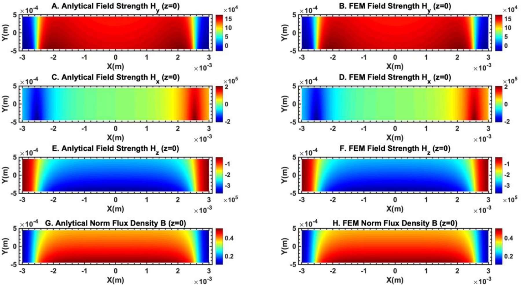
Comparison of the magnetic field distribution obtained from analytical expressions and finite element method simulation (COMSOL Multiphysics version 3.5) showed excellent agreement between the two. (A) and (B) show the y component of the magnetic field strength comparison. The unit of the color bar is A/m. (C) and (D) show the x component of the magnetic field strength comparison. The unit of the color bar is A/m. (E) and (F) show the z component of the magnetic field strength comparison. The unit of the color bar is A/m. (G) and (H) show the comparison of the magnetic flux density norm. The unit of the color bar is T. The plane of the field distribution is at z = 0 (center of the microchannel in the z direction).

Figure 4.

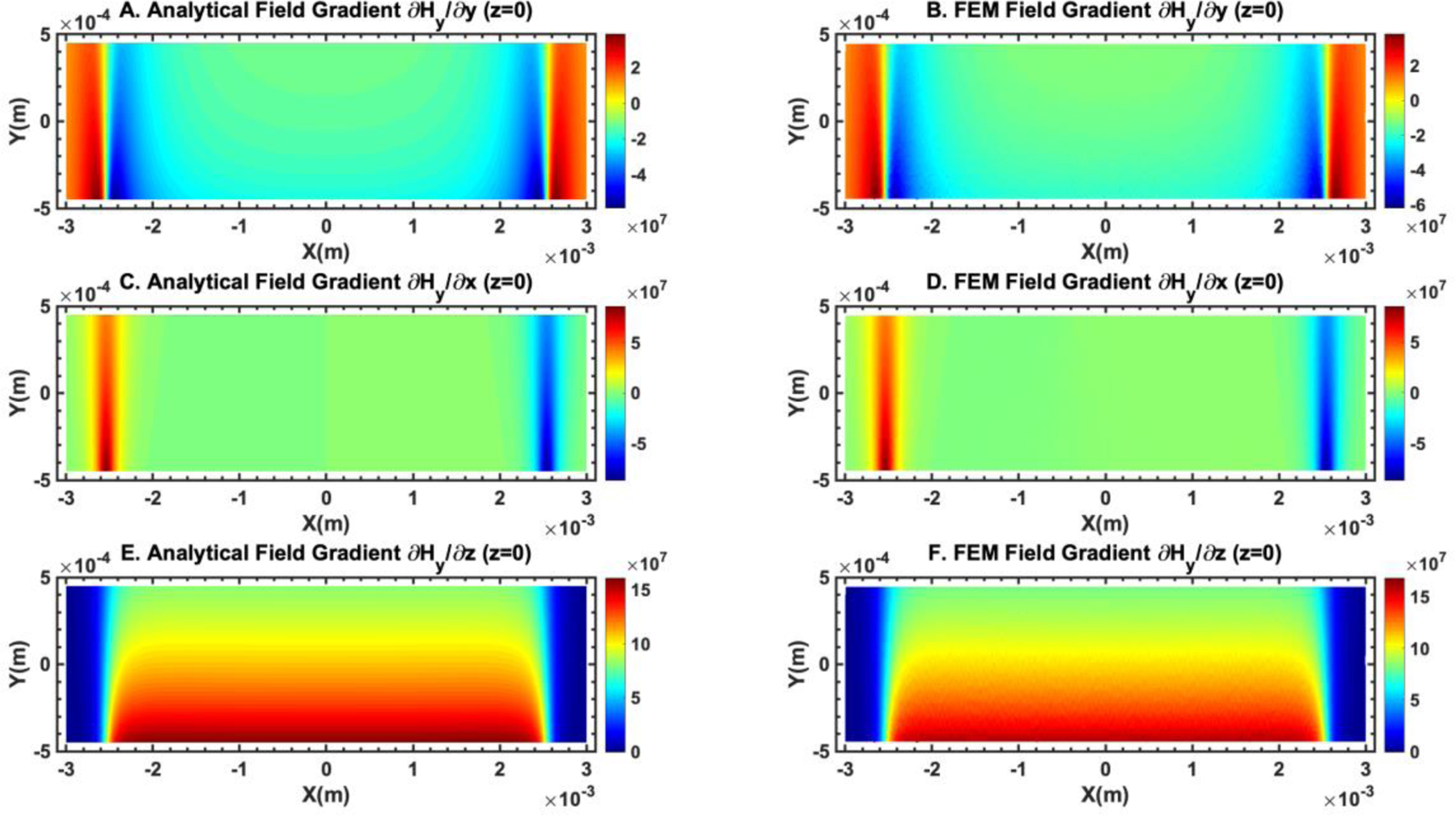
Comparison of the gradient of the magnetic field obtained from analytical expressions and finite element method simulation (COMSOL Multiphysics version 3.5) showed good agreement between the two. (A) and (B) show the comparison of $\partial H_y/\partial y$. The unit of the color bar is A²/m. (C) and (D) show the comparison of $\partial H_y/\partial x$. The unit of the color bar is A²/m. (E) and (F) show the comparison of $\partial H_y/\partial z$. The unit of the color bar is A²/m. The plane of the field distribution is at z = 0 (center of the microchannel in the z direction).

(3). Measurement and approximation of ferrofluid viscosity

The viscosity of a ferrofluid which consists of a suspension of magnetic solids is greater than that of the carrier medium. In the case of no external magnetic field, the ferrofluid viscosity $\eta$ can be related to the viscosity of the carrier medium ${\eta }_0$ and the volume fraction of magnetic materials $\varphi$ using a two-constant expression,³⁶

$$\eta =\frac{{\eta }_0}{1+a\varphi +b{\varphi }^2}$$ (44)

where a and b are the two constants to be determined by fitting experimental data to this expression. We measured the viscosity of the ferrofluid used in this study under no external magnetic field and fitted them to this expression in Figure 2D.

$$\eta =\frac{1.108\times {10}^{-3}}{1-127.3\varphi +4505{\varphi }^2}$$ (45)

In the case of strong magnetic field presence, magnetic nanoparticles in ferrofluids tend to align to the field direction and form rigid chains, which leads to an increase in the overall viscosity. The change of ferrofluid viscosity $\Delta \eta$ due to the magnetic field can be related to the field by³⁶

$$\frac{\Delta \eta }{\eta }=\frac{3}{2}\varphi \frac{0.5\alpha L(\alpha )}{1+0.5\alpha L(\alpha )}{\text{sin}}^2\beta$$ (46)

where $L(\alpha )$ and $\alpha$ are Langevin function and its parameter defined in Eqs. (38) and (39), $\beta$ is the angle between the ferrofluid vorticity and the local magnetic field. The maximum value $\Delta \eta$ can be estimated by

$${\left(\frac{\Delta \eta }{\eta }\right)}_{\text{max}}=\frac{3}{2}\varphi$$ (47)

For diluted ferrofluids such as the one used in this study, its volume fraction of magnetic solids is on the order of 0.1%. As a result, the maximum change in the ferrofluid viscosity due to local magnetic field is negligible for diluted ferrofluids. We used the analytical expression of the ferrofluid viscosity in iFCS optimization.

Optimization of the iFCS

As we discussed above, three primary operating parameters affecting the CTC separation performance of the iFCS devices included sample processing throughput (sample flow rates), ferrofluid concentration (volume fraction of magnetic materials in the ferrofluid), and gradient of applied magnetic fields. Our goal of optimizing these parameters was to obtain a set of device operating parameters that would result in maximal spatial separation of unlabeled CTCs and magnetic bead labeled WBCs at a high sample processing throughput. The analytical model we developed in the previous section provided estimates of the effects from the parameters. First, we tested the validity of the analytical model using experimentally obtained beads’ trajectories. We compared simulated trajectories of microbeads from the model with experimental ones, by imaging 15.0-μm-diameter diamagnetic beads and 11.8-μm-diameter magnetic beads (measured volume fraction of magnetic materials: 0.73% (v/v), see supplementary information) in an iFCS device. This allowed us to compare the difference between the model and experiments. In this process, we defined the deflection of beads in the y-direction of the microchannel (see Figure 1F for coordinates), denoted as Y, and the separation distance between the two types of beads, denoted as ΔY. The simulation results were carried out using three parameters including sample processing throughput (10 – 600 μL/min, or 6 – 36 mL/h), ferrofluid concentration (volume fraction of magnetic materials in ferrofluids, 0 – 1.0%, v/v), and gradient of applied magnetic field flux density (20 – 280 T m⁻¹). These parameters were chosen for practical purposes. Firstly, the sample processing throughput range corresponded to the clinically relevant target. In order to separate a sufficient number of circulating tumor cells, a significant amount of blood samples (typically 10 mL) needed to be processed within 1 hour to obtain sufficient tumor cells. Our chosen sample processing throughput range (10 – 600 μL/min, or 6 – 36 mL/h) would make the eventually optimized throughput clinically relevant. Secondly, ferrofluid concentration (volume fraction of magnetic materials in ferrofluids) was chosen to be 0 – 1.0% (v/v) because it approximately corresponded to the volume fraction of magnetic materials in the labeled white blood cells in this study. Lastly, gradient of applied magnetic flux density range was chosen to be 20 – 280 T/m, because it was determined by the residual magnetic flux density of the permanent magnet, and the distance between the magnet and the microchannel. For the permanent magnet used in this paper, which had 1.33 T residual magnetic flux density (Figure 2D), and the approximate distance between the magnet surface and microchannel edge, which is ~1 mm, we estimated that the gradient of applied magnetic flux density was 132 T/m at the center of the microchannel. Therefore we chose a range of 20 – 280 T/m for the optimization study. Our goal of optimization was to maximize the separation of diamagnetic beads from magnetic beads, which translated to maximizing both Y and ΔY simultaneously. We extracted Y and ΔY at the end of the microchannel and used them to compare simulation and experimental results.

We first studied the sample processing throughput of the iFCS device. Simulation and experimental results agreed well, and (Figure 5A) showed a monotonically decreasing trend for ΔY as the throughput increased. Simulation (Figure 5D) and experimental results (Figure 5G) indicated highly dispersed trajectories for the 11.8 μm magnetic beads, and well-deflected trajectories for 15.0 μm diamagnetic beads. The highly dispersed trajectories of magnetic beads were likely due to the randomly distributed starting positions of these beads at the start of the iFCS microchannel. The second parameter we studied was the ferrofluid concentration. We observed that a higher ferrofluid concentration resulted in larger magnetic force on diamagnetic beads and a larger deflection in their y-direction. Meanwhile, magnetic beads’ deflection changed its direction and magnitude in their y-direction as ferrofluid concentration increased. This was because the magnetic force on the beads depended on the contrast of magnetization between the magnetic beads and ferrofluids. When the contrast of magnetization between the magnetic beads and ferrofluids became smaller, which happened as the ferrofluid concentration approached that of magnetic beads (0.73 % v/v) (Figures 5E and 5H), separation distance ΔY became smaller because of the decreased magnetic force (Figure 5B). The last parameter we studied was the magnetic field gradient, whose value could be adjusted by the distance between the magnet and the microchannel. Figure 5C and 5F indicated that in both simulation and experiments, the deflection for both beads increased when the magnetic field gradient increased. This was because the magnetic force on beads was proportional to the gradient of the magnetic field strength. In summary, through comparing the simulation and experimental results, we concluded that both of them followed the same trends in all three parametric studies (sample processing throughput, ferrofluid volume concentration, gradient of magnetic field flux density).

Figure 5.

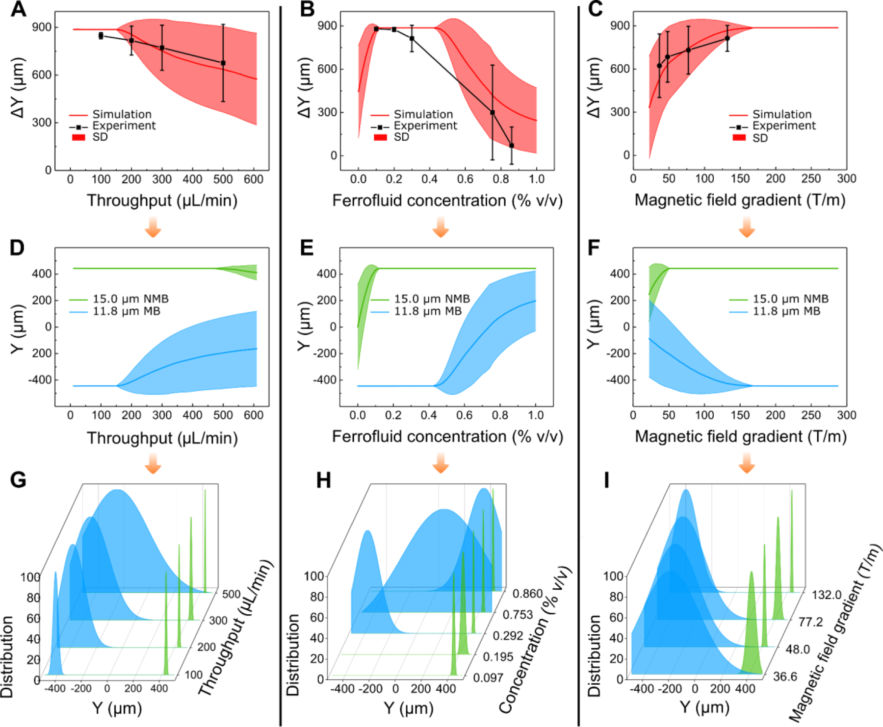
Optimization of iFCS device via simulation and beads validation. Parametric studies of beads’ deflection Y and separation distance ΔY between magnetic and diamagnetic beads were conducted with three parameters: (A)&(D)&(G) sample processing throughput (sample flow rate), (B)&(E)&(H) volumetric concentration of magnetic materials in the ferrofluid, and (C)&(F)&(I) gradient of magnetic flux density. Ferrofluid concentration was constant at 0.292% (v/v) for the results in (A)&(D)&(G)& (C)&(F)&(I), gradient of magnetic flux density was 132 T m⁻¹ (at the center of the microchannel) for (A)&(D)&(G), and sample processing throughput was 100 μL/min for (B)&(E)&(H)& (C)&(F)&(I). (A)&(B)&(C) were the comparison between simulated and experimentally obtained separation distance at the end of the iFCS device. (D)&(E)&(F) were simulated beads trajectories with randomly distributed starting positions at the inlet of the device. (G)&(H)&(I) were experimentally obtained normalized bead distributions at the outlets of the device. SD in (A)&(B)&(C) represented standard deviation of bead trajectory distribution.

We further validated the iFCS model with multiple beads separation experiments in order to simulate a more realistic scenario in CTC separation where unlabeled tumor cells were polydispersed in their physical sizes and labeled WBCs were magnetic. For this purpose, we used a mixture of three diamagnetic beads (diameters: 5.7, 8.0, and 20.3 μm) to represent the polydispersity of CTCs in blood, and one magnetic beads (diameter: 11.8 μm, magnetic volume fraction: 0.73%) to represent labeled WBCs. The mixture of these beads was spiked into the ferrofluid and separated in the iFCS device at variable sample throughput (flow rates) and ferrofluid concentration. Figures 6A and 6B shows the comparison between the simulated and experimental separation distance between each diamagnetic bead and magnetic bead. Figure 6A shows all three diamagnetic beads could be fully separated from the magnetic beads at a sample flow rate of 100 μL/min. Figure 6B shows a 0.049% ferrofluid concentration that resulted in the full separation of 8 μm diamagnetic beads and 11.8 μm magnetic beads. Possible sources of discrepancies between simulation and experiments in Figures 6 included random starting positions of beads at the beginning of the iFCS device and large variation of magnetic contents in commercial magnetic beads. Figures 6D–F shows the experimental images of the separation of a mixture of 20.3 and 8.0 μm (red fluorescence) diamagnetic beads and 11.8 μm (yellow fluorescence) magnetic beads in the iFCS device. Full separation of the diamagnetic and magnetic beads was achieved at the end of the device (Figure 6F). Based on the above studies, we determined the following operating parameters for an optimized iFCS device which led to maximal separation distance of beads: 100 μL/min (6 mL/hour) as sample processing throughput, 0.049% as volume concentration of magnetic materials in ferrofluids, and 132 T/m as gradient of magnetic field flux density.

Figure 6.

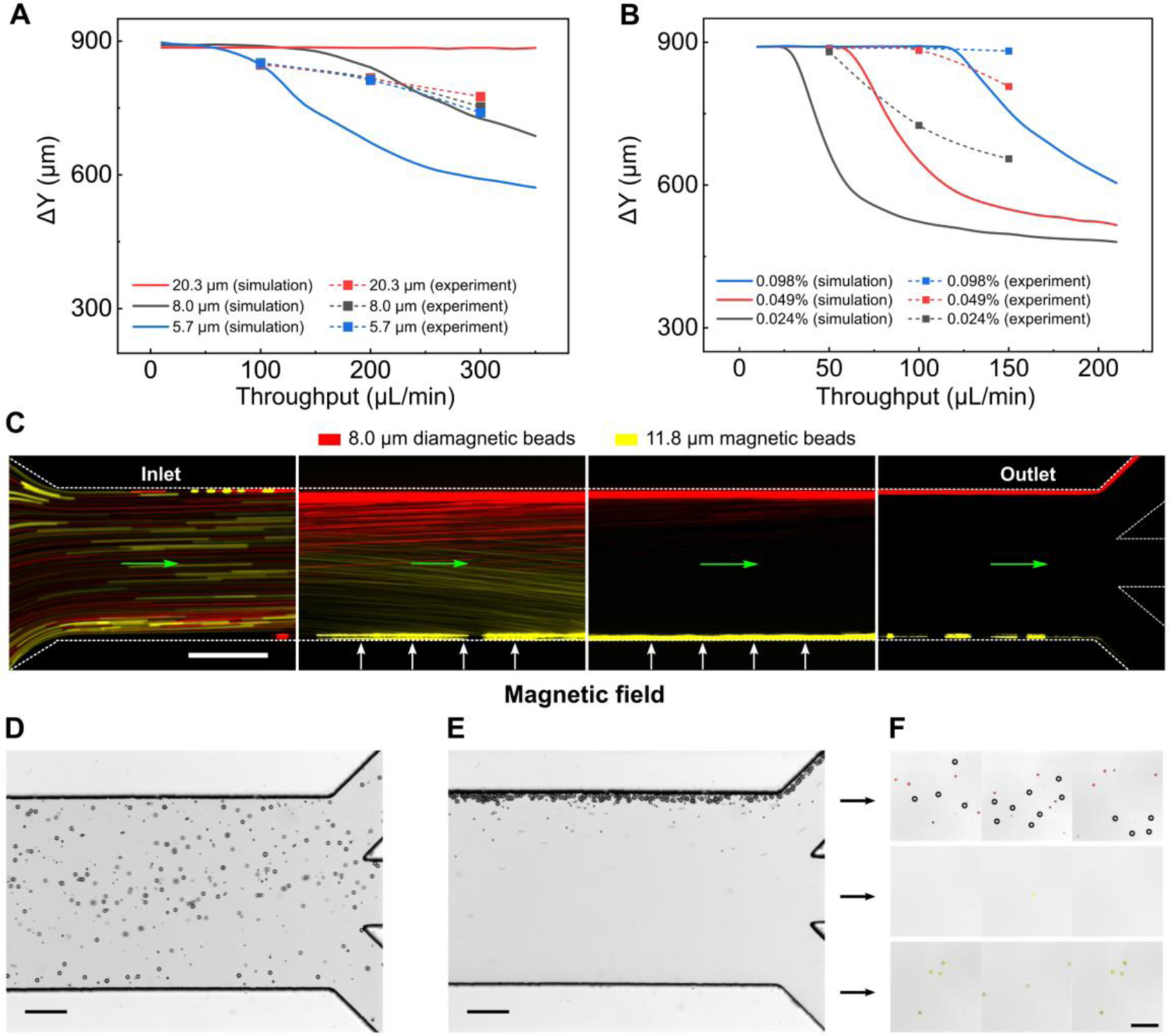
Multiple sized bead separation in an iFCS device. (A) Averaged separation distance (number of experiments n=3) between diamagnetic beads and magnetic beads. Diamagnetic beads (20.3 μm, 8.0 μm, and 5.7 μm) and magnetic beads (11.8 μm) were spiked into a 0.292% (v/v) ferrofluid at variable sample throughput (10 – 350 μL/min). (B) Averaged separation distance (number of experiments n=3) between 8.0 μm diamagnetic beads and 11.8 μm magnetic beads at ferrofluid concentration between 0.01% and 0.1%, and throughput between 10 and 210 μL/min. (C) Bead trajectories of 8.0 μm diamagnetic beads (red) and 11.8 μm magnetic beads (yellow) at sample throughput of 100 μL/min. A ferrofluid with a concentration of 0.049% (v/v) was used. The green arrows indicate the flow direction. (D) In absence of magnetic fields, all beads (20.3 and 8.0 μm diamagnetic beads, and 11.8 μm magnetic beads) were randomly distributed in the channel at the outlets. (E) When magnetic fields were present, diamagnetic beads (20.3 and 8.0 μm) flowed into the top outlet. Majority of magnetic beads (11.8 μm) flowed into bottom outlet. (F) Image of collected beads from outlets. The red fluorescent signal was from 8.0 μm diamagnetic beads and the yellow fluorescent signal was from 11.8 μm magnetic beads. Gradient of magnetic field flux density was 132 T/m (at the center of the microchannel) in all figures. Scale bars in (C-F): 200 μm.

Validation of iFCS with spiked cancer cells.

With the optimized operating parameters determined through the previous section, we validated the iFCS using WBCs spiked with cancer cells. iFCS can separate cancer cells independent of their physical sizes and surface antigen based on its operating principle and previous beads studies. To demonstrate its size-independent capability, we chose a total of 9 cell lines including one prostate cancer (PC-3), three breast cancer (MCF7, MDA-MB-231, HCC1806), two non-small cell lung cancer (H1299, H3122), two small cell lung cancer (DMS79, H69), and one canine melanoma cancer (Jones). These cancer cell lines had different size distributions, as showed in measured size profiles in Figure 7A. We observed that all cancer cells were polydispersed in their physical sizes, and there was a size overlap between cancer cell lines and WBCs. This made the separation of cancer cells from WBCs based on size difference alone challenging. Therefore in iFCS we employed a strategy that integrated both “diamagnetophoresis” and “magnetophoresis” for the separation of cancer cells regardless of the size distribution of cancer cells. In order to label the WBCs and deplete them, we used a combination of two leukocyte surface biomarkers to label WBCs: CD45 and CD66b antibody. Figure 7B shows that the mean number of magnetic beads (dynabeads) on the surface of WBCs was 25 ± 8 (mean ± standard deviation), with more than 99.8% of WBCs labeled. The minimum volume fraction of magnetic content in WBCs was 0.032%, corresponding WBCs that were labeled with just one magnetic bead (Figure 7C). Based on the cancer cell size distribution and the labeling efficiency of WBCs, we modified the optimized ferrofluid concentration to be 0.029% so that WBCs labeled with only one magnetic bead could be separated from cancer cells. Based on the beads simulation and experimental results (Figure 6A), the optimized throughput remained to be 100 μL/min, and the gradient of magnetic field flux density remained to be 132 T/m to collect cancer cells that were larger than 5.7 μm in diameter.

Figure 7.

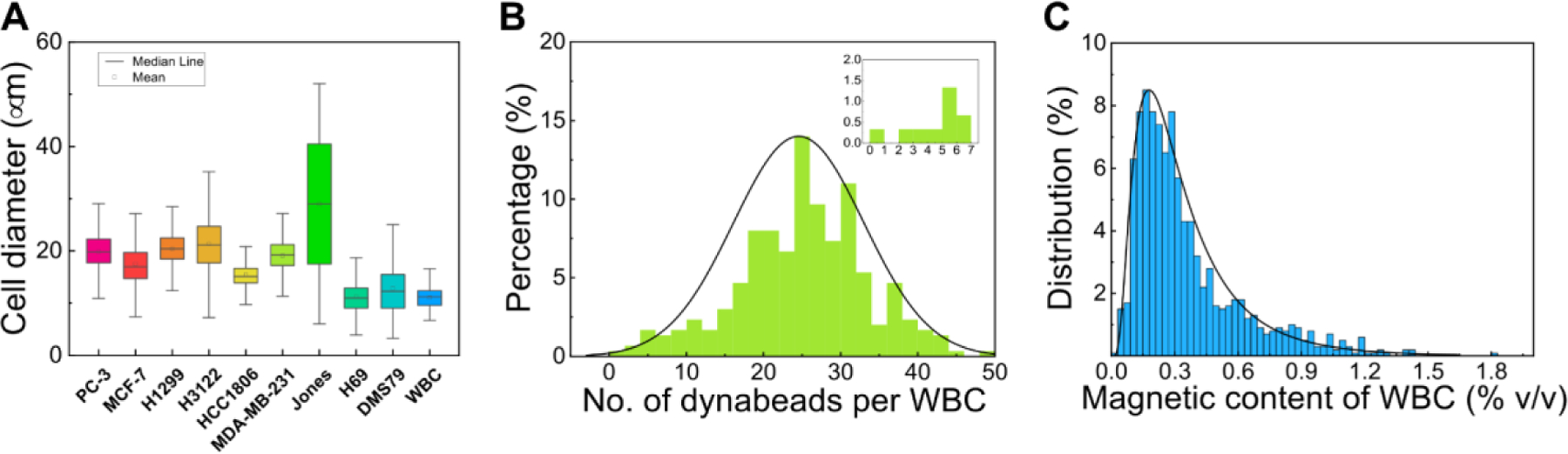
Measurement of physical size distribution of cancer cells and magnetic labeling of WBCs. (A) Size distribution of cancer cell lines – Prostate cancer (PC-3), Breast cancer (MCF7, MDA-MB-231, HCC1806), non-small cell lung cancer (H1299, H3122), small cell lung cancer (DMS79, H69), and white blood cells from healthy donors. (B) Percentage of labeled WBCs versus the number of magnetic beads (dynabeads) per WBC (n=500). The average dynabeads per WBC was 25 ± 8 (mean ± standard deviation). The insert was the percentage of WBCs labeled with <= 7 dynabeads. More than 99.5% of WBCs were labeled with more than one dynabeads (C) Percentage of labeled WBCs versus their volumetric fraction of magnetic materials. The volume fraction of magnetic materials in a WBC (${\varphi }_{WBC}=n\times D_{\mathit{\text{Dynabead}}}^3\times {\varphi }_{\mathit{\text{Dynabead}}}/(D_{WBC}^3+n\times D_{\mathit{\text{Dynabead}}}^3)$ was calculated based on the following parameters – number of Dynabeads on each WBC (n), the diameter of the WBC in question ($D_{WBC}$), the volume fraction of magnetic materials in each Dynabead (${\varphi }_{\mathit{\text{Dynabead}}}$), and the diameter of the Dynabead ($D_{\mathit{\text{Dynabead}}}$). The volume fraction of magnetic materials in each Dynabead (${\varphi }_{\mathit{\text{Dynabead}}}$) was provided by the manufacturer to be 11.5% (v/v), and the diameter of the Dynabead ($D_{\mathit{\text{Dynabead}}}$) is 1.05 μm. The number of Dynabeads on each WBC (n) was determined experimentally from image analysis, and the diameter of the WBC in question ($D_{WBC}$) was calculated using their surface areas with the assumption that cells were spherical.

Using optimized operation parameters in an iFCS device, we studied cancer cell separation using 9 cancer cell lines that have distinct size distributions. Separation performance including cancer cell recovery rate, WBC depletion, recovered cancer cell viability, and sample processing throughput were used to evaluate iFCS. A typical cancer cell separation process is shown in Figure 8A, in which ~100 cancer cells labeled with CellTracker green fluorescence were spiked into 1 mL of human whole blood and flowed through an iFCS device under optimized conditions. Cells were randomly distributed at the channel inlet, then started to deflect towards the top of the channel when they entered the magnetic field region, and were completely deflected into the top outlet at the end of the channel (Figure 8A, top and middle panels). WBCs labeled with DAPI (blue fluorescence, Figure 8A, bottom panel) were either trapped at the bottom side of the channel due to their strong interaction with magnetic fields or flowed into the bottom outlet at the end of the channel. There trapped WBCs in the microchannel had little effect on the flow profile and cancer cell separation performance when processing less than 3 mL of blood. We first measured the size profiles of cancer cells before and after the separation. Figure 8B and Table 1 show the average diameters of three cancer cells (MCF7, MDA-MB-231, and H1299) had no significant change, demonstrating iFCS’s capability to separate cancer cells regardless of their size distribution. We then determined the WBC contamination in the iFCS output. Figure 8C shows the average number of magnetic beads enumerated on the surface of WBCs found in the device output depended on the ferrofluid concentrations. The use of 0.029% (v/v) ferrofluid resulted in the average number of beads on the contaminating WBC were 0.5. We determined experimentally that there were ~1,620 WBCs contamination (99.973% depletion) after processing 1 mL of blood. We also determined iFCS’s ability in recovering cancer cells from spiked samples. Figure 8D shows the recovery rates of 99.68 ± 0.56%, 97.92 ± 0.96%, 97.59 ± 1.01 %, 98.75 ± 1.43 %, 99.35 ± 0.56 %, 98.71 ± 0.58%, 98.58 ± 0.87%, 94.99 ± 1.22%, 95.93 ± 1.34% for PC-3, MCF7, MDA-MB-231, HCC1806, H1299, H3122, Jones, DMS79, H69 cell lines, respectively. It is worth noting that two small cell lung cancer cells, DMS79 and H69, whose size distribution was very close to that of WBCs, can be recovered in iFCS with a recovery rate of ~95%. We characterized the robustness of the iFCS recovery rate at variable spike ratios using PC-3 prostate cancer cells. Figure 8E shows a corresponding recovery rate of 98.8%. Figure 8F shows that for PC3 prostate cancer cells the iFCS processing had little effect on their cellular viability.

Figure 8.

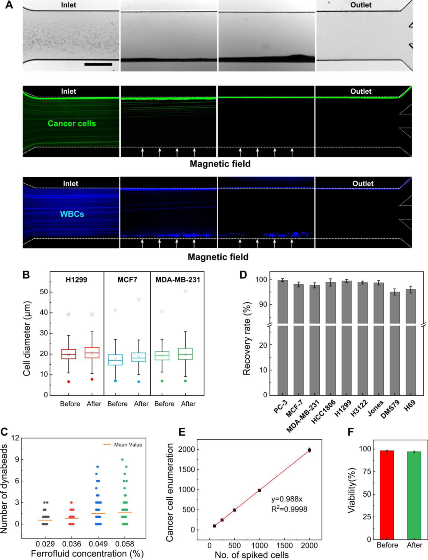
Validation of iFCS using spike-in cancer cells. (A) Visualization of a typical separation process of cancer cells and WBCs in one iFCS device. ~10⁵ PC-3 cancer cells and ~10⁶ WBCs were spiked into a ferrofluid with a concentration of 0.029% (v/v) prior to the separation. The concentration of cancer cells was chosen to be much higher than CTC concentration in blood circulation for better visualization of the separation process. The cellular mixture was processed in the iFCS device at a throughput of 100 μL/min; the gradient of magnetic flux density was 132 T/m at the center of the microchannel. Bright-field and fluorescent images of cancer cells and WBCs were shown here. Green fluorescence was from PC-3 cancer cells and blue fluorescence was from the WBCs. Scale bar: 500 μm. (B) Comparison of size distributions of H1299, MCF7, and MDA-MB-231 cancer cells (n=3000) before and after iFCS separation showed no significant changes. (C) Magnetic beads enumeration on the WBCs found in the iFCS output at different concentrations of ferrofluids. (D) Recovery rate for different cancer cell lines (spike ratio: ~100 cells spiked per 1mL of blood). Recovery rate of 99.68 ± 0.56%, 97.92 ± 0.96%, 97.59 ± 1.01 %, 98.75 ± 1.43 %, 99.35 ± 0.56 %, 98.71 ± 0.58%, 98.58 ± 0.87%, 94.99 ± 1.22%, 95.93 ± 1.34% and were achieved for PC-3, MCF7, MDA-MB-231, HCC1806, H1299, H3122, Jones, DMS79, H69 cell lines, respectively. Error bars indicate standard deviation of three experiments. (E) Recovery of spiked PC-3 cancer cells at variable ratios (spike ratios: 100, 250, 500, 1000, and 2000 PC-3 cells per one milliliter of blood). An average recovery rate of 98.8% (linear fit, R² = 0.9998) was calculated for PC-3 cancer cells. (F) Short-term viability of recovered PC-3 cancer cells comparison before and after the iFCS separation. Cell viability of PC-3 cells before and after separation was determined to be 98.72 ± 0.44%, and 97.25 ± 0.75%.

Table 1.

Distributions of physical diameters of three types of cancer cells before and after iFCS processing.

Cancer cell line	Minimum diameter (spiked, μm)	Minimum cell diameter (collected, μm)	average diameter (spiked, μm)	average diameter (collected, μm)	P value, t-test
MCF7	7.12	6.55	17.48 ± 4.28	18.76 ± 5.31	0.0001
MDA-MB-231	7.05	7.01	19.10 ± 3.57	19.92 ± 4.59	0.0001
H1299	6.64	7.77	19.89 ± 4.64	20.44 ± 4.86	0.017

Validation of iFCS with canine/human cancer patient blood.

As a clinical validation of iFCS method, we first validated it with blood samples obtained from one canine cancer patient under an approved protocol (University of Georgia, CRC-525). For this canine patient, peripheral blood was collected from the patient with newly diagnosed osteosarcoma (stage II) before initiation of treatment. Blood sample was processed with iFCS devices within 2 hours of blood draw. A total of 3 mL of blood sample was processed from the patient. After iFCS processing, cytopathological staining of collected cells was performed in order to identify CTCs and WBCs (Figure 9A). These cells were concentrated and stained using the Alkaline Phosphatase stain (ALP), which was commonly used for cytopathology analysis of clinical samples.^{42, 43} Isolated cells were inspected by a cytopathologist and the number of CTCs found were enumerated. CTCs were identified using a combination of the following criteria: (1) cells that demonstrated positive cytoplasmic ALP staining; (2) large cells with high nuclear to cytoplasmic (N:C) ratio; (3) cells that were 4–5 times the size of a WBC.^{42, 43} Figure 9A shows ALP-stained CTCs and WBCs separated from the canine patient. These CTCs were ALP-negative, but their morphology confirmed that they were CTCs. A total of 5 CTCs were separated from 3 mL blood sample for this patient. This canine patient was presented with stage II osteosarcoma disease, which was a high-grade tumor with vascular invasion on histopathology but without evidence of clinically detectable metastases at diagnosis. However, this patient was euthanized three months later due to multifocal metastasis to the vertebral column. This information provided evidence that the cells identified by iFCS were likely CTCs.

Figure 9.

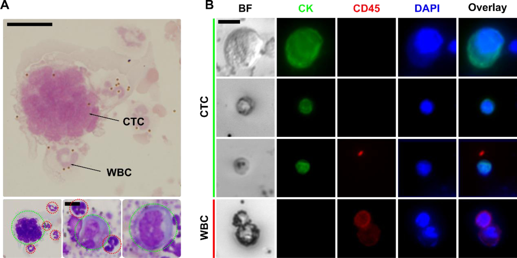
Validation of iFCS with canine and human cancer patients’ blood sample. (A) Cytopathological staining of isolated CTC from a canine patient with stage II osteosarcoma. CTCs were indicated by dotted green circles; WBCs were indicated by dotted red circles. Scale bar: 10 μm. (B) Bright-field and immunofluorescence images of 3 selected CTCs and 1 WBC separated from 2 human patients with stage IV breast cancer. Four channels were used in immunofluorescence staining, including the CTC marker cytokeratin (CK, green), leukocyte marker CD45 (red), and nucleus marker DAPI (blue). Cells were identified as CTC if the staining pattern is CK+/CD45−, WBCs were identified as CK−/CD45+. Scale bar: 10 μm.

We also validated iFCS with blood samples obtained from two human cancer patients with stage IV breast cancer under an approved protocol (University of Georgia, STUDY00005431). For these two human patients, peripheral blood was collected from them before initiation of treatment. Blood sample was processed with iFCS devices within 2 hours of blood draw. 3 mL of blood sample was processed from each patient. After iFCS processing, cells separated from these two patients’ samples were immunofluorescence stained with cytokeratin (CK), leukocyte marker CD45, and nuclear marker DAPI (Figure 9B). CTCs were identified as CK+/CD45−/DAPI+, while WBCs were identified as CK−/CD45+/DAPI+. Based on the immunostaining criteria, 72 and 21 CTCs were identified in 3 mL blood sample from the two breast cancer patients’ samples respectively.

Comparison of iFCS to existing technologies

CTC separation has been under intensive research for the past decade and a myriad of labeled-based and label-free technologies were developed based on either the use of specific tumor cell markers or the use of physical features of tumor cells. While the emphasis of this paper is to present the fundamental theory of iFCS, we compared iFCS to a total of ⁴³ other CTC separation technologies in order to evaluate iFCS’s performance (see supplementary information table). We chose to use 4 performance metrics for the comparison, including cell-processing throughput (volume of blood processed per hour), CTC recovery rate from spiked samples at low spiking concentration (1–100 cells/mL), purity of CTCs after separation (or contaminating cells carryover), and viability of separated CTCs. These metrics had significant effects on the downstream analysis or expansion of CTCs after their separation, and were often used in reviews of existing methods to evaluate performance of CTC separation.^{1, 14} The performance metrics of iFCS reported in this paper were: (1) a recovery rate of 98.8% at low CTC occurrence rate (~100 cells mL⁻¹); (2) a WBC carryover of 1620 cells for every 1 milliliter blood processed, (3) a blood processing throughput of 6 mL h⁻¹, and (4) minimally affected cell viability after separation (before: 98.72 ± 0.44%; after: 97.25 ± 0.75%). Firstly, we noted that the recovery rate of the iFCS (98.8%) was high among existing methods, approaching that of monolithic CTC-iChip (99.5%).⁴⁴ iFCS could recover almost all CTCs from the blood sample because it didn’t select CTCs using surface markers but rather depleted contaminating WBCs. This way, any potential CTCs which didn’t present the specific markers used to deplete WBCs on their surface were enriched and preserved, leading to a complete recovery of CTCs. Secondly, we noted that purity of separated CTCs from iFCS was lower than some of existing technologies, including the ones based on inertial forces (Vortex⁴⁵), immunoaffinity (Magsweeper,⁴⁶ CTC-Chip,⁴⁷ GEDI,⁴⁸ GEM-Chip⁴⁹), immunomagnetic positive methods (Magnetic Sifter,⁵⁰ SIM-chip,⁵¹ and CTC-μChip⁵²). Levels of CTC purity from iFCS depended on the efficiency of WBC labeling and depletion, as well as the ferrofluid concentration. In this paper, we used a combination of two antibodies (CD45 and CD66b) to target WBCs, which resulted in a carryover of 1620 WBCs for every one milliliter of whole blood processed. In order to increase the purity of CTCs and reduce the WBC carryover, more WBC targeting antibodies could be used in combination to increase the efficiency of labeling and depletion. The ferrofluid concentration (volume fraction of magnetic materials in the ferrofluid) could also be further decreased so that large WBCs attached with just one magnetic bead could be depleted to increase the purity. Thirdly, we noted that the cell processing throughput of iFCS was 6 mL/hour, which was lower than a few high throughput methods, including Vortex,⁴⁵ and ^LPCTC-iChip.⁵³ Finally, we noted that the red blood cell lysis step in iFCS could potentially cause CTC loss in processing patient samples. In summary, iFCS had the advantages of high recovery in CTC separation, but had the drawbacks of high WBC carryover and the need of red blood cells lysis in its current form.

Conclusion

In this paper, we presented the fundamental theory of integrated ferrohydrodynamic cell separation (iFCS), a scheme that could separate circulating tumor cells (CTCs) from blood independent of surface antigen and physical size of cells. Relying on a magnetic liquid medium, ferrofluid, whose magnetization could be tuned by adjusting its magnetic volume concentration, iFCS integrated both diamagnetophoresis of CTCs and magnetophoresis of blood cells together in order to separate the two. We developed governing equations of iFCS in order to effectively guide its optimization process for specific cell separation applications. In this process, we determined three critical parameters that affected iFCS’s cell separation performance. These parameters included the sample flow rate, volumetric concentration of magnetic materials in the ferrofluid, and the gradient of the magnetic flux density. We studied these coupled parameters in an experimentally validated analytical model and determined optimized parameters in an iFCS device with simple geometry. These parameters led to a high recovery CTC separation in both spiked samples and clinical samples.

Experimental section

Custom-made biocompatible ferrofluid and determination of its physical and magnetic properties.

A water-based ferrofluid is synthesized by chemical co-precipitation method based on previous protocol.^{54, 55} The magnetic properties of the ferrofluid were measured by a vibrating sample magnetometer (VSM; MicroSense, LLC, Lowell, MA). Measurement data from VSM were fitted to a Langevin function in order to extract physical and magnetic properties of this ferrofluid, including its particle diameter distribution and volume fraction of magnetic materials. Transmission electron microscopy (TEM; FEI Corp., Eindhoven, the Netherlands) was also used to determine the size and morphology of the maghemite nanoparticles. The average diameter of nanoparticles in ferrofluid was measured to be 10.91 ± 4.87 nm. This measured particle diameter was consistent with the mean diameter calculated from VSM measurement (10.8 nm). The viscosity of this ferrofluid was measured with a compact rheometer (Anton Paar, Ashland, VA) at room temperature. This ferrofluid was made isotonic and had a 7.0 pH, coated with a neutral surfactant, and was colloidally stable for up 10 months’ storage at room temperature.

Modeling and simulation

Bead and cell trajectories in the iFCS optimization process were simulated in MATLAB (MathWorks, Natick, MA) by balancing the magnetic force and hydrodynamic viscous drag force in the laminar flow condition. Full set of equations and solver are in the supplementary information. Estimated Reynold’s number was 0.3 – 3.8 Magnetic field distributions were obtained from analytical expression in MATLAB, as well as three-dimensional simulation in COMSOL Multiphysics (COMSOL Inc, Burlington, MA).

Magnetic field measurement and approximation

The remanent magnetization of a neodymium permanent magnet (50.8 × 12.7 × 12.7 mm, L × W × H; N52, K&J Magnetics, Pipersville, PA) used in the iFCS device were measured with a Gauss meter (Model 5080, F.W. BELL, Orlando, FL). The setup of the measurement was shown in the supplementary information. The measured value of the remanent magnetization of the magnet was 1,055,693 A/m, and the residual magnetic flux density of the magnet was 1.33 T. The measured remanent magnetization of the magnet was then used in Equations (41–43) to approximate the magnetic field distributions in the microchannel. In experiments, the permanent magnet was placed 1 – 4 mm away from the microchannel (surface of the magnet to channel wall) to adjust the field distribution inside the channel.

Microbeads calibration.

Polystyrene microbeads with diameters of 20.3 μm (Bangs Laboratories Inc., Fishers, IN), 15.0 μm and 8.0 μm (Thermo Fisher Scientific Inc., Fremont, CA), and 5.7 μm (Polysciences, Inc., Warminster, PA) were used in iFCS validation. Diamagnetic beads are mixed with magnetic beads with a diameter of 11.8 μm (Spherotech Inc, Lake Forest, IL) at a concentration of 1×10⁴ particles per 1mL in ferrofluid.

iFCS device fabrication.

Microfluidic devices were made of PDMS by replicating the master mold which was fabricated using standard photolithography methods. The thickness of the channel was measured by a profilometer (Veeco Instruments, Chadds Ford, PA). One neodymium permanent magnet (50.8 × 12.7 × 12.7 mm, L × W × H; N52, K&J Magnetics, Pipersville, PA) was embedded 1 mm away from the PDMS channel with their magnetization direction vertical to the channel. Devices were flushed with 70% ethanol and then primed with 1× PBS supplemented with 0.5% (w/v) BSA and 2mM EDTA (Thermo Fisher Scientific, Waltham, MA) before each use.

Cell culture.

Eight human cancer cell lines including three breast cancer cell lines (MCF7, MDA-MB-231, and HCC1806), two non-small cell lung cancer (NSCLC) cell lines (H1299 and H3122), two small cell lung cancer (SCLC) cell lines (H69 and DMS79) and one prostate cancer cell line (PC-3) were obtained from ATCC (Manassa, VA). One canine melanoma cell line (Jones) was obtained from Dr. Meichner’s lab at the University of Georgia. Cell cultures followed the manufacturing instructions. MCF7 and MDA-MB-231 cells were cultured in Dulbecco’s modified eagle medium (DMEM; Life Technologies, Carlsbad, CA) with 10% (v/v) FBS, 1% (v/v) penicillin/streptomycin solution and 0.1 mM NEAA (Life Technologies, Carlsbad, CA). Other cell lines were cultured in RPMI-1640 medium (Life Technologies, Carlsbad, CA) supplemented with 10 % (v/v) FBS and 1% (v/v) penicillin/streptomycin solution. All the cell lines were cultured at 37 °C under a humidified atmosphere with 5% CO₂ supplied.

Cancer cells staining and preparation.

Cancer cell lines were washed with phosphate-buffered saline (1× PBS; Life Technologies, Carlsbad, CA) and released with a 0.05% trypsin-EDTA solution (Life Technologies, Carlsbad, CA) before each use. 2 μM CellTracker Green (Life Technologies, Carlsbad, CA) was used to fluorescently stain cancer cells. The CellTracker working solution was replaced with culture medium after 30 minutes. Cells are counted with a hemocytometer (Hausser Scientific, Horsham, PA) and diluted to 1 × 10⁴ cells per mL with culture medium. The exact number of cells in the diluted solution was measured twice with a Nageotte counting chamber (Hausser Scientific, Horsham, PA). Different numbers of cancer cells (100, 500, 1000, 2000, 10000) and 1 million WBCs were spiked into 1 mL ferrofluid.

Cancer cell recovery rate calculation.

Collected cells from iFCS outlets were stained with 2 μM DAPI (Thermo Fisher Scientific, Waltham, MA) to identify the nucleated cell. The number of cells was counted with a Nageotte counting chamber. Cells with CellTracker signal was identified as cancer cells, while other cells with DAPI signal was classified as WBC contamination. The recovery rate was calculated by the number of collected cancer cells / number of spiked cancer cells.

Cell size measurement.

Cells were deposited onto microscope slides and imaged with a microscope in bright field mode. Images of cells were analyzed by the ImageJ software. The effective diameter of the cells was calculated using their surface areas with the assumption that cells were spherical.

Live subject statement

All experiments in this study were performed in compliance with the regulations of the United States Office for Human Research Protections, the University of Georgia Human Subjects Office, and the University of Georgia Clinical Research Committee and Hospital Board. Human whole blood was obtained from healthy donors following a protocol approved by the Institutional Review Board (IRB) at the University of Georgia (STUDY00005431). Human cancer patient blood samples were obtained from the University Cancer and Blood center (Athens, GA) following a protocol approved by the Institutional Review Board (IRB) at the University of Georgia (STUDY00005431). Informed consent was obtained for the healthy donors and cancer patient participants. Canine cancer patient blood samples were obtained from the University of Georgia Veterinary Teaching Hospital (Athens, GA) following an protocol approved by the University of Georgia Clinical Research Committee and Hospital Board (CRC-525).

Human patient blood processing.

The sample was loaded into a 3mL syringe (BD, Franklin Lakes, NJ,) followed by processing with the iFCS device at a throughput of 100 μL/min. After separation, the iFCS device was flushed by 1× PBS at 500 μL/min for 20 minutes to remove cells in the outlet reservoir. Collected cells were preserved in RPMI-1640 medium (Life Technologies, Carlsbad, CA) supplemented with 10 % (v/v) FBS and 1% (v/v) penicillin/streptomycin solution. Collected cells were then concentrated and immobilized onto poly-L-lysine coated glass slides with a customized cell collection chamber.

Canine patient blood processing.

The labeled cells were resuspended win 0.029% ferrofluid and collected using the same process described above.

WBC labeling.

Human sample:

Human whole blood was obtained from healthy donors following a protocol approved by the Institutional Review Board (IRB) at the University of Georgia (STUDY00005431). The amount of biotinylated antibodies and magnetic beads required were calculated based on the WBC count. 100 fg per WBC for anti-human CD45 (BioLegend, San Diego, CA) and anti-human CD66b (Life Technologies, Carlsbad, CA) were used. WBCs were labeled with magnetic beads (Dynabeads Myone streptavidin T1, Life Technologies, Carlsbad, CA). Dynabeads were washed twice with 0.01% TWEEN 20 in PBS, then washed with 0.1% BSA in PBS and resuspended in PBS. Whole blood was firstly labeled with antibodies for 30 minutes and lysed by RBC lysis buffer (EBioscience, San Diego, CA) for 7 minutes at room temperature. Cell mixtures were centrifuged for 5 minutes at 800×g and the pellet was suspended in PBS with dynabeads. Cells and Dynabeads were incubated for 25 minutes on the rocker. Ferrofluid and 0.1% (v/v) Pluronic F-68 non-ionic surfactant (Thermo Fisher Scientific, Waltham, MA) were added into the mixture to achieve the same volume with whole blood.

Canine sample:

Canine whole blood was obtained from healthy dogs from UGA Veterinary Teaching Hospital (Athens, GA) following an approved protocol at the University of Georgia (CRC-525). 100 fg per WBC for anti-canine CD45 (Thermo Fisher Scientific, Waltham, MA) and anti-canine CD4 (R&D Systems, Minneapolis, MN) were used. Dynabeads labeling and washing process was the same as in human sample processing.

CTC identification.

Human cancer sample:

Collected cells were fixed with 4% (w/v) PFA for 10 minutes and subsequently permeabilized with 0.2% (v/v) Triton X-100 in PBS for 10 minutes. Cells were then blocked by 0.5% (w/v) BSA in PBS for 30 minutes. After blocking nonspecific binding sites, cells were immunostained with primary antibodies including anti-cytokeratin (Milteryi Biotec, Auburn, CA) and anti-CD45 (Abcam, Cambridge, MA). Nuclei were counterstained with DAPI (Thermo Fisher Scientific Inc., Fremont, CA). After immunofluorescence staining, cells were washed with PBS and stored at 4 °C or imaged with a fluorescence microscope.

Canine cancer sample:

Collected cells were stained with Alkaline Phosphatase Staining Kit (Millipore Sigma, Burlington, MA) following the manufacturer’s protocol. Briefly, the sample was stained with Wright’s Giemsa (Millipore Sigma, Burlington, MA) for initial cytologic diagnosis following incubation with ALP staining for 60 minutes. Samples were then rinsed with tap water, air-dried, and inspected by a cytopathologist. Neutrophils from a previously stained horse blood smear were used as the positive control. CTCs were expected to be ALP positive, but some CTCs are ALP negative and required morphological confirmation. Based on the combination of a high nuclear to cytoplasmic ratio, large size, and nuclear morphology, cells were identified as CTCs.

References

- 1.Poudineh M, Sargent EH, Pantel K and Kelley SO, Nat Biomed Eng, 2018, 2, 72–84. [DOI] [PubMed] [Google Scholar]
- 2.Alix-Panabieres C and Pantel K, Nat Biomed Eng, 2017, 1. [Google Scholar]
- 3.Massague J and Obenauf AC, Nature, 2016, 529, 298–306. [DOI] [PMC free article] [PubMed] [Google Scholar]
- 4.Krebs MG, Metcalf RL, Carter L, Brady G, Blackhall FH and Dive C, Nat Rev Clin Oncol, 2014, 11, 129–144. [DOI] [PubMed] [Google Scholar]
- 5.Heitzer E, Haque IS, Roberts CES and Speicher MR, Nat Rev Genet, 2019, 20, 71–88. [DOI] [PubMed] [Google Scholar]
- 6.Ma N and Jeffrey SS, Science, 2020, 367, 1424–1425. [DOI] [PubMed] [Google Scholar]
- 7.Chaffer CL and Weinberg RA, Science, 2011, 331, 1559–1564. [DOI] [PubMed] [Google Scholar]
- 8.Lambert AW, Pattabiraman DR and Weinberg RA, Cell, 2017, 168, 670–691. [DOI] [PMC free article] [PubMed] [Google Scholar]
- 9.Cheung KJ and Ewald AJ, Science, 2016, 352, 167–169. [DOI] [PMC free article] [PubMed] [Google Scholar]
- 10.Riethdorf S, Fritsche H, Muller V, Rau T, Schindibeck C, Rack B, Janni W, Coith C, Beck K, Janicke F, Jackson S, Gornet T, Cristofanilli M and Pantel K, Clin Cancer Res, 2007, 13, 920–928. [DOI] [PubMed] [Google Scholar]
- 11.Romiti A, Raffa S, Di Rocco R, Roberto M, Milano A, Zullo A, Leone L, Ranieri D, Mazzetta F, Medda E, Sarcina I, Barucca V, D’Antonio C, Durante V, Ferri M, Torrisi MR and Marchetti P, J Gastrointest Liver, 2014, 23, 279–284. [DOI] [PubMed] [Google Scholar]
- 12.Bidard FC, Peeters DJ, Fehm T, Nole F, Gisbert-Criado R, Mavroudis D, Grisanti S, Generali D, Garcia-Saenz JA, Stebbing J, Caldas C, Gazzaniga P, Manso L, Zamarchi R, de Lascoiti AF, De Mattos-Arruda L, Ignatiadis M, Lebofsky R, van Laere SJ, Meier-Stiegen F, Sandri MT, Vidal-Martinez J, Politaki E, Consoli F, Bottini A, Diaz-Rubio E, Krell J, Dawson SJ, Raimondi C, Rutten A, Janni W, Munzone E, Caranana V, Agelaki SA, Almici C, Dirix L, Solomayer EF, Zorzino L, Johannes H, Reis JS, Pantel K, Pierga JY and Michiels S, Lancet Oncol, 2014, 15, 406–414. [DOI] [PubMed] [Google Scholar]
- 13.Alix-Panabieres C and Pantel K, Nat Rev Cancer, 2014, 14, 623–631. [DOI] [PubMed] [Google Scholar]
- 14.Chen Y, Li P, Huang PH, Xie Y, Mai JD, Wang L, Nguyen NT and Huang TJ, Lab Chip, 2014, 14, 626–645. [DOI] [PMC free article] [PubMed] [Google Scholar]
- 15.Poudineh M, Aldridge P, Ahmed S, Green BJ, Kermanshah L, Nguyen V, Tu C, Mohamadi RM, Nam RK, Hansen A, Sridhar SS, Finelli A, Fleshner NE, Joshua AM, Sargent EH and Kelley SO, Nat Nanotechnol, 2017, 12, 274–+. [DOI] [PubMed] [Google Scholar]
- 16.Cheng YH, Chen YC, Lin E, Brien R, Jung S, Chen YT, Lee W, Hao Z, Sahoo S, Min Kang H, Cong J, Burness M, Nagrath S, M SW and Yoon E, Nat Commun, 2019, 10, 2163. [DOI] [PMC free article] [PubMed] [Google Scholar]
- 17.Sahai E, Nat Rev Cancer, 2007, 7, 737–749. [DOI] [PubMed] [Google Scholar]
- 18.Nieto MA, Huang RY, Jackson RA and Thiery JP, Cell, 2016, 166, 21–45. [DOI] [PubMed] [Google Scholar]
- 19.Dasgupta A, Lim AR and Ghajar CM, Mol Oncol, 2017, 11, 40–61. [DOI] [PMC free article] [PubMed] [Google Scholar]
- 20.Warkiani ME, Khoo BL, Wu LD, Tay AKP, Bhagat AAS, Han J and Lim CT, Nat Protoc, 2016, 11, 134–148. [DOI] [PubMed] [Google Scholar]
- 21.Renier C, Pao E, Che J, Liu HE, Lemaire CA, Matsumoto M, Triboulet M, Srivinas S, Jeffrey SS, Rettig M, Kulkarni RP, Di Carlo D and Sollier-Christen E, npj Precision Oncology, 2017, 1, 15. [DOI] [PMC free article] [PubMed] [Google Scholar]
- 22.Ozkumur E, Shah AM, Ciciliano JC, Emmink BL, Miyamoto DT, Brachtel E, Yu M, Chen PI, Morgan B, Trautwein J, Kimura A, Sengupta S, Stott SL, Karabacak NM, Barber TA, Walsh JR, Smith K, Spuhler PS, Sullivan JP, Lee RJ, Ting DT, Luo X, Shaw AT, Bardia A, Sequist LV, Louis DN, Maheswaran S, Kapur R, Haber DA and Toner M, Sci Transl Med, 2013, 5. [DOI] [PMC free article] [PubMed] [Google Scholar]
- 23.Zhao WJ, Liu Y, Jenkins BD, Cheng R, Harris BN, Zhang WZ, Xie J, Murrow JR, Hodgson J, Egan M, Bankey A, Nikolinakos PG, Ali HY, Meichner K, Newman LA, Davis MB and Mao LD, Lab on a Chip, 2019, 19, 1860–1876. [DOI] [PMC free article] [PubMed] [Google Scholar]
- 24.Alix-Panabieres C and Pantel K, Clin Chem, 2013, 59, 110–118. [DOI] [PubMed] [Google Scholar]
- 25.Zhao W, Cheng R, Jenkins BD, Zhu T, Okonkwo NE, Jones CE, Davis MB, Kavuri SK, Hao Z, Schroeder C and Mao L, Lab Chip, 2017, 17, 3097–3111. [DOI] [PMC free article] [PubMed] [Google Scholar]
- 26.Zhao W, Cheng R, Lim SH, Miller JR, Zhang W, Tang W, Xie J and Mao L, Lab Chip, 2017, 17, 2243–2255. [DOI] [PMC free article] [PubMed] [Google Scholar]
- 27.Zhao W, Zhu T, Cheng R, Liu Y, He J, Qiu H, Wang L, Nagy T, Querec TD, Unger ER and Mao L, Adv Funct Mater, 2016, 26, 3990–3998. [DOI] [PMC free article] [PubMed] [Google Scholar]
- 28.Zhao W, Cheng R, Miller JR and Mao L, Adv Funct Mater, 2016, 26, 3916–3932. [DOI] [PMC free article] [PubMed] [Google Scholar]
- 29.Xuan X, Micromachines, 2019, 10, 744. [DOI] [PMC free article] [PubMed] [Google Scholar]
- 30.Pamme N, Lab Chip, 2006, 6, 24–38. [DOI] [PubMed] [Google Scholar]
- 31.Gijs MA, Lacharme F and Lehmann U, Chem Rev, 2010, 110, 1518–1563. [DOI] [PubMed] [Google Scholar]
- 32.Hejazian M, Li W and Nguyen NT, Lab Chip, 2015, 15, 959–970. [DOI] [PubMed] [Google Scholar]
- 33.Zhao W, Liu Y, Jenkins BD, Cheng R, Harris BN, Zhang W, Xie J, Murrow JR, Hodgson J, Egan M, Bankey A, Nikolinakos PG, Ali HY, Meichner K, Newman LA, Davis MB and Mao L, Lab Chip, 2019, 19, 1860–1876. [DOI] [PMC free article] [PubMed] [Google Scholar]
- 34.Cheng R, Zhu T and Mao L, Microfluidics and Nanofluidics, 2014, 16, 1143–1154. [Google Scholar]
- 35.Zhu T, Lichlyter DJ, Haidekker MA and Mao L, Microfluidics and Nanofluidics, 2011, 10, 1233–1245. [Google Scholar]
- 36.Rosensweig RE, Ferrohydrodynamics, Cambridge University Press, Cambridge, 1985. [Google Scholar]
- 37.Brenner H, Chem Eng Sci, 1961, 16, 242–251. [Google Scholar]
- 38.Lin BH, Yu J and Rice SA, Phys Rev E, 2000, 62, 3909–3919. [DOI] [PubMed] [Google Scholar]
- 39.Unni M, Uhl AM, Savliwala S, Savitzky BH, Dhavalikar R, Garraud N, Arnold DP, Kourkoutis LF, Andrew JS and Rinaldi C, ACS Nano, 2017, 11, 2284–2303. [DOI] [PMC free article] [PubMed] [Google Scholar]
- 40.Luigjes B, Woudenberg SMC, de Groot R, Meeldijk JD, Torres Galvis HM, de Jong KP, Philipse AP and Erné BH, The Journal of Physical Chemistry C, 2011, 115, 14598–14605. [Google Scholar]
- 41.Furlani E, Permanent magnet and electromechanical devices, Academic Press, New York, 2001. [Google Scholar]
- 42.Barger A, Graca R, Bailey K, Messick J, de Lorimier LP, Fan T and Hoffmann W, Vet Pathol, 2005, 42, 161–165. [DOI] [PubMed] [Google Scholar]
- 43.Ryseff JK and Bohn AA, Vet Clin Pathol, 2012, 41, 391–395. [DOI] [PubMed] [Google Scholar]
- 44.Fachin F, Spuhler P, Martel-Foley JM, Edd JF, Barber TA, Walsh J, Karabacak M, Pai V, Yu M, Smith K, Hwang H, Yang J, Shah S, Yarmush R, Sequist LV, Stott SL, Maheswaran S, Haber DA, Kapur R and Toner M, Sci Rep-Uk, 2017, 7. [DOI] [PMC free article] [PubMed] [Google Scholar]
- 45.Sollier E, Go DE, Che J, Gossett DR, O’Byrne S, Weaver WM, Kummer N, Rettig M, Goldman J, Nickols N, McCloskey S, Kulkarni RP and Di Carlo D, Lab Chip, 2014, 14, 63–77. [DOI] [PubMed] [Google Scholar]
- 46.Talasaz AH, Powell AA, Huber DE, Berbee JG, Roh KH, Yu W, Xiao WZ, Davis MM, Pease RF, Mindrinos MN, Jeffrey SS and Davis RW, P Natl Acad Sci USA, 2009, 106, 3970–3975. [DOI] [PMC free article] [PubMed] [Google Scholar]
- 47.Nagrath S, Sequist LV, Maheswaran S, Bell DW, Irimia D, Ulkus L, Smith MR, Kwak EL, Digumarthy S, Muzikansky A, Ryan P, Balis UJ, Tompkins RG, Haber DA and Toner M, Nature, 2007, 450, 1235–U1210. [DOI] [PMC free article] [PubMed] [Google Scholar]
- 48.Gleghorn JP, Pratt ED, Denning D, Liu H, Bander NH, Tagawa ST, Nanus DM, Giannakakou PA and Kirby BJ, Lab on a Chip, 2010, 10, 27–29. [DOI] [PMC free article] [PubMed] [Google Scholar]
- 49.Sheng WA, Ogunwobi OO, Chen T, Zhang JL, George TJ, Liu C and Fan ZH, Lab on a Chip, 2014, 14, 89–98. [DOI] [PMC free article] [PubMed] [Google Scholar]
- 50.Earhart CM, Hughes CE, Gaster RS, Ooi CC, Wilson RJ, Zhou LY, Humke EW, Xu LY, Wong DJ, Willingham SB, Schwartz EJ, Weissman IL, Jeffrey SS, Neal JW, Rohatgi R, Wakeleebe HA and Wang SX, Lab on a Chip, 2014, 14, 78–88. [DOI] [PMC free article] [PubMed] [Google Scholar]
- 51.Kim J, Cho H, Han S-I and Han K-H, Analytical chemistry, 2016, 88, 4857–4863. [DOI] [PubMed] [Google Scholar]
- 52.Cho H, Kim J, Jeon C-W and Han K-H, Lab on a Chip, 2017, 17, 4113–4123. [DOI] [PubMed] [Google Scholar]
- 53.Mishra A, Dubash TD, Edd JF, Jewett MK, Garre SG, Karabacak NM, Rabe DC, Mutlu BR, Walsh JR and Kapur R, Proceedings of the National Academy of Sciences, 2020, 117, 16839–16847. [DOI] [PMC free article] [PubMed] [Google Scholar]
- 54.Zhao W, Zhu T, Cheng R, Liu Y, He J, Qiu H, Wang L, Nagy T, Querec TD and Unger ER, Advanced functional materials, 2016, 26, 3990–3998. [DOI] [PMC free article] [PubMed] [Google Scholar]
- 55.Zhao W, Cheng R, Lim SH, Miller JR, Zhang W, Tang W, Xie J and Mao L, Lab on a Chip, 2017, 17, 2243–2255. [DOI] [PMC free article] [PubMed] [Google Scholar]
Associated Data
This section collects any data citations, data availability statements, or supplementary materials included in this article.