An improved SIR model describing the epidemic dynamics of the COVID-19 in China

Abstract

In this letter, an improved SIR (ISIR) model is proposed, to analyze the spread of COVID-19 during the time window 21/01/2020–08/02/2021. The parameters can be extracted from an inverse problem of the ISIR to assess the risk of COVID-19. This study identifies that the cure rate is 0.05 and the reproduction number is 0.4490 during the time interval. The prediction values demonstrates high similarity to the reported data. The results indicate that the disease had been under control in China.

Introduction

On December 2019, the Corona Virus Disease 2019 (COVID-19) confirmed case was reported in Wuhan, Hubei, China. The disease COVID-19 has become the deadliest infectious disease in the world soon [1], [2]. COVID-19 is quite different from the previous SARS, and it is a totally new coronavirus that has not been previously identified. As of 26/01/2021, 100 360 cases of COVID-19 were officially confirmed in China, including 4815 deaths. During the same time window, more than 99.79 million cases of COVID-19 were confirmed worldwide, including about 2.1 million deaths. It has evolved into a global public health incident and caused huge loss of life in the world.

In 2020, techniques about COVID-19 have become an active and flouring research topic. In terms of COVID-19, different models are used to estimate the key features of the disease such as the incubation period, transmissibility, asymptomatic, severity, and likely impact of different public health interventions. Among those models, the SIR-type model, the Logistic model, the nonlinear fitting model due to the exponential nature of growth of the epidemic, and extrapolation models are commonly adopted by using different biological and social processes. SIR (Susceptible–Infected–Recovered) shares several characteristics with models of population dynamics and conceptual lumped models in hydrology. The basic model of the SIR is listed as follows:

$$\left\{\begin{array}{c}{S}^{\prime }=-\beta SI,\hfill \\ I^{\prime }=\beta SI-\gamma I,\hfill \\ R^{\prime }=\gamma I,\hfill \end{array}\right)$$ (1)

where $\beta$ is the transmission rate and $\gamma$ the recuperation rate. Although this model is nonlinear, it can be analytically solved.

This model simulates the temporal evolution of some compartments of the population [3], [4]. Some examples refer to applications to dengue transmission [5], H5N1 [6], HIV [7] and SARS [8]. It is the basic method to deal with the analysis of the infectious diseases. Therefore, many scholars have developed a number of predicting approaches to the trend forecasting of COVID-19, in the worst affected countries, based on the SIR-type model [9], [10], [11], [12]. However, COVID-19 is quite different from SARS and other infectious diseases, whose trend cannot be simply analyzed by applying the SIR-type model based on other diseases. For example, the transmission probability of the COVID-19 is not a constant during the time interval and the compartment of the total population is more complicated than the one in the basic SIR model, and so on.

Besides the SIR-type model, the Logistic model is often used in regression fitting of time series data due to its simple principle and efficient calculation [13], [14]. In the COVID-19 cases, Logistic growth is characterized by a slow increase in growth at the beginning, fast growth phase approaching the peak of the incidence curve and a slow growth phase approaching the end of the outbreak [15], [16], [17], [18]. The Logistic model originated form the modeling of population growth in ecology. As an improvement on the Malthus population model, in 1838, Pieere Francois Verhulst published the basic model of the Logistic as follows:

$$\frac{dQ}{dt}=rQ(1-\frac{Q}{K})\to Q\left(t\right)=\frac{K}{1+a\times e^{r\times t}},$$ (2)

where $Q$, $r$, $K$ indicate the size of accumulates infected cases, the intrinsic growth and the maximum cases size that the world or country could carry, respectively.

The main weakness of the Logistic model is that it does not consider the spread characteristics. The Logistic model is not the mechanism model. Many feature parameters cannot be obtained by the Logistic model. Due to the imported cases, the maximum cases size cannot be obtained accurately.

The main objective of this paper is to construct a reliable model based on the SIR-type model to analyze and assess the epidemic dynamics of COVID-19 in China. There are two important problems. The first is how to construct the comprehensive mathematical model based on the characteristics of COVID-19. The second problem is how to estimate parameters of the model describing the evolution in the time of the current COVID-19 pandemic. To overcome these two problems, this paper proposes an ISIR model, which subdivides the total population into the following seven compartments: Susceptible, Infected, Recovered, Death, Exposed, Quarantine, and Patients with suspected. They are based on phenomenological laws to describe the transfer of individuals from one class to another. On the other hand, this paper discretizes the differential equation model via a forward-time finite-difference scheme. The parameters of the proposed model are estimated via a minimization problem.

This rest of this paper is structured as follows. In “An improved SIR model for COVID-19”, the continuous and the discrete models are proposed, based on the SIR model. The results on the COVID-19 parameters, obtained by applying our ISIR model, are shown in “An inverse problem of the ISIR and solution algorithm”, and numerical simulations are given in “Simulations, results and conclusions”.

An improved SIR model for COVID-19

The continuous ISIR model

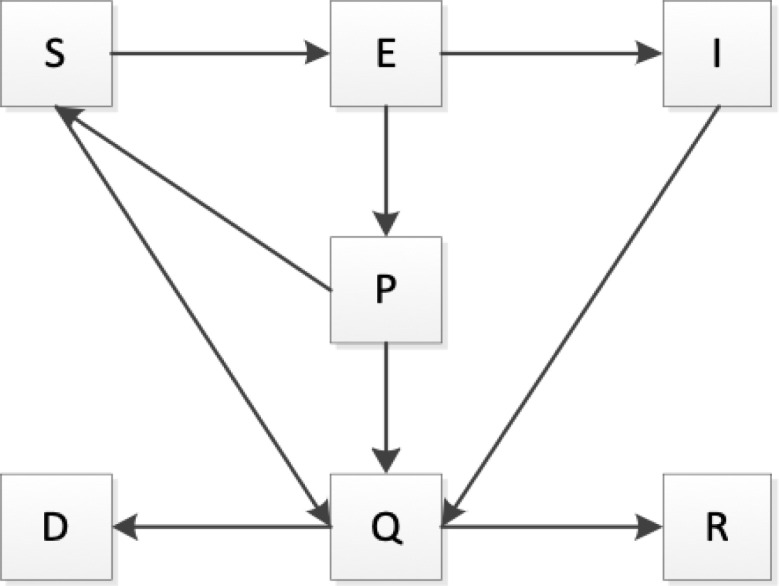
In this subsection, an improved SIR model will be proposed. We start our research by defining the objects involved in the continuous ISIR model considered in this paper. We divide the total population into seven compartments: susceptible individuals in the free environment (S), undiagnosed and non-isolated infectious individuals (I), recovered individuals (R), death individuals (D), free Exposed (E), Confirmed and isolated infectious individuals (Q), and Patients with suspected (P). The transfer relationships between compartments are shown in Fig. 1.

Fig. 1.

Flow chart of the COVID-19 transmission model.

We denote by $ϵ$, $\alpha$ and $\gamma$ the rate latent individuals progressed to the undiagnosed infectious class, the fatality rates related to the pandemic, and recovery rates, respectively. The transfer relationships between class R and other classes can be expressed as follows:

$$R^{\prime }=\gamma Q.$$ (3)

Suspected cases might be misdiagnosed, and the number of the misdiagnosed individuals entering P class is $d_{sp}$ Q. Misdiagnosed suspected cases return to the susceptible class at a rate of $b_{sp}$. We use the function $f(S,E,I,R)$ to measure the number of the suspected individuals transferring into the exposed class. Therefore, the transfer relationships between class S and other classes can be expressed as follows:

$$S^{\prime }=-f(S,E,I,R)-d_{sp}Q+b_{sp}P.$$ (4)

We denote by $d_{ep}$ the rate of the tracked and free exposed individuals diagnosed as suspected cases. We assume that diagnosed and confirmed individuals are strictly isolated and could not further infect others. We denote the impulse function ${\delta }_{e}ta(x-x_0)$ and the delta function $\delta (x-x_0)$ below:

$${\delta }_{\eta }(x-x_0)=\left\{\begin{array}{c}\frac{1}{2\eta },x_0-\eta <x<x_0+\eta ,\hfill \\ 0,\text{otherwise},\hfill \end{array}\right)$$ (5)

$$\delta (x-x_0)=\underset{\eta \to 0}{lim}{\delta }_{\eta }(x-x_0).$$ (6)

We denote by $m_i$ the number of imported cases at time $t_i$. Therefore, the transfer relationships between class E and other classes can be expressed as follows:

$$E^{\prime }=f(S,E,I,R)-(ϵ+d_{ep})E+\sum _{i=1}^m{h}_i\delta (t-t_i).$$ (7)

Non-isolated infectious individuals are diagnosed and confirmed at a rate of $d_{ip}$. Therefore, the transfer relationships between class I and other classes can be expressed as follows:

$$I^{\prime }=ϵE-d_{ip}I.$$ (8)

Suspected individuals are further diagnosed and confirmed at a rate of $d_{pq}$. Therefore, the transfer relationships between class P, class Q and other classes can be expressed as follows:

$$P^{\prime }=d_{ep}E+d_{sp}Q-(b_{sp}+d_{pq})P,$$ (9)

$$Q^{\prime }=d_{pq}P+d_{ip}I-(\alpha +\gamma )Q.$$ (10)

We only consider the deaths caused by COVID-19. Therefore, the transfer relationships between class D and other classes can be expressed as follows:

$$D^{\prime }=\alpha Q.$$ (11)

We denote by $C$ the contracted rate, which we assume to be the same in the exposed class and the infectious class:

$$f(S,E,I,R)=({\beta }_{E}CE+{\beta }_{I}CI)\frac{S}{S+E+I+R}=\frac{{\beta }_{I}CS}{S+E+I+R}(\frac{{\beta }_E}{{\beta }_I}E+I).$$ (12)

The ${\beta }_E$ and ${\beta }_I$ mean the individuals transmission rates in the exposed class and the infectious class, respectively, and ${\beta }_E\ll {\beta }_I$. We denote the $\beta \left(t\right)$ to be the transmission probability at time $t$ as follows:

$$\beta \left(t\right)\triangleq \frac{{\beta }_{I}CS}{S+E+I+R}=\frac{f\left(t\right)}{\frac{{\beta }_E}{{\beta }_I}E+I}.$$ (13)

A discrete ISIR model

A discrete model is a simple forward-time finite-difference discretization of Eqs. (1). For $n\in Z$, we denote the discrete time steps, at a uniform spacing $\Delta t=1$ day, in agreement with the sampling of the available date set on COVID-19 pandemic, by $t_n=n\Delta t$. Data for this study are the total cumulative confirmed cases, recovered cases and total deaths cases, active cases, suspected cases of COVID-19 in China from 30/01/2020 to 08/02/2021. This real-time data was compiled by the National Health Commission of People’s Republic of China and made available on the website at the time we started to conduct our study [19].

We describe the precise methodology used to find reasonably good approximation of the function $\beta \left(t\right)$. According to the experiences of experts, the average duration of new infectious individuals keeping in the free environments is 10 days and the average duration of individuals keeping in the exposed class is 7 days. Therefore, the approximation of the function $\beta \left(n\right)$ is given as follows:

$$\beta \left(n\right)=\frac{F(n+10)}{\sum _{i=0}^{6}F(n+i)+k\times \sum _{i=7}^{9}F\left(n\right)},$$ (14)

where $F\left(n\right)$ is the total confirmed cases reported at time $t_n$, and $k=\frac{{\beta }_E}{{\beta }_I}$.

In order to more comprehensively use the reported data to estimate unknown model parameters, the required discrete model is given as follows:

$$\left\{\begin{array}{c}S(n+1)=S\left(n\right)-\beta \left(n\right)(kE\left(n\right)+I\left(n\right))-d_{sp}Q\left(n\right)+b_{sp}P\left(n\right),\hfill \\ E(n+1)=E\left(n\right)-ϵE\left(n\right)+\beta \left(n\right)(kE\left(n\right)+I\left(n\right))-d_{ep}E\left(n\right)\hfill \\ +\sum _{i=1}^m{h}_i\delta (n-i),\hfill \\ I(n+1)=I\left(n\right)+ϵE\left(n\right)-d_{ip}I\left(n\right)-\alpha I\left(n\right),\hfill \\ P(n+1)=P\left(n\right)+d_{ep}E\left(n\right)+d_{sp}Q\left(n\right)-b_{sp}P\left(n\right)-d_{pq}P\left(n\right),\hfill \\ Q(n+1)=Q\left(n\right)+d_{pq}P\left(n\right)+d_{iq}I\left(n\right)-\alpha Q\left(n\right)-\gamma Q\left(n\right),\hfill \\ R(n+1)=R\left(n\right)+\gamma Q\left(n\right),\hfill \\ D(n+1)=D\left(n\right)+\alpha Q\left(n\right).\hfill \end{array}\right)$$ (15)

We denote by $X\left(n\right)={(S\left(n\right),E\left(n\right),I\left(n\right),P\left(n\right),Q\left(n\right),R\left(n\right),D\left(n\right))}^T$ the vector of numbers of all classes at time $t_n$. The matrix $A\left(n\right)$ is constructed to express the transfer cases from $t_n$ to $t_{n+1}$, and the matrix $B\left(n\right)$ is constructed to express the imported cases at time $t_n$:

$$A\left(n\right)=\left[\begin{array}{ccccccc}\hfill 1\hfill & \hfill -\beta \left(n\right)k\hfill & \hfill -\beta \left(n\right)\hfill & \hfill b_{sp}\hfill & \hfill -dsp\hfill & \hfill 0\hfill & \hfill 0\hfill \\ \hfill 0\hfill & \hfill 1-ϵ+\beta \left(n\right)k-d_{ep}\hfill & \hfill \beta \left(n\right)\hfill & \hfill 0\hfill & \hfill 0\hfill & \hfill 0\hfill & \hfill 0\hfill \\ \hfill 0\hfill & \hfill ϵ\hfill & \hfill 1-d_{ip}-\alpha \hfill & \hfill 0\hfill & \hfill 0\hfill & \hfill 0\hfill & \hfill 0\hfill \\ \hfill 0\hfill & \hfill d_{ep}\hfill & \hfill 0\hfill & \hfill 1-d_{sp}-d_{pq}\hfill & \hfill d_{sp}\hfill & \hfill 0\hfill & \hfill 0\hfill \\ \hfill 0\hfill & \hfill 0\hfill & \hfill d_{iq}\hfill & \hfill d_{pq}\hfill & \hfill 1-\alpha -\gamma \hfill & \hfill 0\hfill & \hfill 0\hfill \\ \hfill 0\hfill & \hfill 0\hfill & \hfill 0\hfill & \hfill 0\hfill & \hfill \gamma \hfill & \hfill 1\hfill & \hfill 0\hfill \\ \hfill 0\hfill & \hfill 0\hfill & \hfill 0\hfill & \hfill 0\hfill & \hfill \alpha \hfill & \hfill 0\hfill & \hfill 1\hfill \end{array}\right],$$

$$B\left(n\right)=\left[\begin{array}{c}\hfill 0\hfill \\ \hfill h_n\hfill \\ \hfill 0\hfill \\ \hfill 0\hfill \\ \hfill 0\hfill \\ \hfill 0\hfill \end{array}\right].$$

We can obtain the number of each class at time $t_{n+1}$ from the number at time $t_n$:

$$X(n+1)=A\left(n\right)X\left(n\right)+B\left(n\right).$$ (16)

$X\left(0\right)$ is the initial condition. $Q\left(0\right)$, $D\left(0\right)$ and $R\left(0\right)$ are the active cases, total deaths cases and recovered cases reported on 31/01/2020. $E\left(0\right)$, $I\left(0\right)$, $P\left(0\right)$ are the unknown model parameters whose values are not reported. They can be obtained from the solution of an inverse problem.

An inverse problem of the ISIR and solution algorithm

The reported active cases, total recovered cases and total deaths cases at time $t_i$ are denoted by $w_i$, $y_i$ and $k_i$. Thus, the reported active cases series, the total recovered cases series and the total deaths cases series read $W=[w_1,\dots w_i,\dots ]$, $K=[k_1,\dots ,k_i,\dots ]$ and $Y=[y_1,\dots ,y_i,\dots ]$.

The estimated values of the initial condition of class I and class P are $\widehat{I\left(0\right)}$ and $\widehat{P\left(0\right)}$, the estimated value of the initial condition of the susceptible cases can be obtained as follows:

$$\widehat{S\left(0\right)}=N-\widehat{I\left(0\right)}-\widehat{P\left(0\right)}-D\left(0\right)-Q\left(0\right)-R\left(0\right).$$ (17)

The estimated values of model parameters are denoted by $\widehat{ϵ}$, $\widehat{d_{ep}}$, $\widehat{d_{ip}}$, $\widehat{\alpha }$, $\widehat{\gamma }$, $\widehat{d_{pg}}$. These estimated parameters substituted in Eqs. (15), the estimated values of the active cases $\widehat{Q\left(n\right)}$, total deaths cases $\widehat{D\left(n\right)}$ and the recovered cases $\widehat{R\left(n\right)}$ at time $t_{n+1}$ can be obtained, based on the initial condition, according to Eq. (16).

The misfit between model predictions and the target values is computed by the following functions:

$$m_1=\sum {|w_i-\widehat{Q\left(i\right)}|}^2$$ (18)

$$m_2=\sum {|y_i-\widehat{R\left(i\right)}|}^2$$ (19)

$$m_3=\sum {|k_i-\widehat{D\left(i\right)}|}^2$$ (20)

This inverse problem is the multi-objective optimization problem. The final function is the sum of above three functions, each of which considers one of the reference quantities:

$$op=\sum _{i=1}^3{m}_i.$$ (21)

The unknown model parameters can be write $up$ as a vector:

$$up=[I\left(0\right),P\left(0\right),ϵ,d_{ep},d_{ip},\alpha ,\gamma ,d_{pg}].$$ (22)

These model parameters are fixed before the simulation and obtained from the solution of the underlying inverse problem. The objective of the model calibration is to find the parameter values which best fit the reference data in the given time interval:

$$u{p}^{\ast }=argminop.$$ (23)

By the next-generation matrix model, we obtain the effective reproduction number of the model (15), which is given by Eq. (23):

$$R_0=\frac{\beta \left(t\right)(ϵ+k(\alpha +d_{ip}))}{(ϵ+d_{ep})(\alpha +d_{ip})}.$$ (24)

$R_0>1$ means the occurrence of infectious disease becomes more frequent, and $R_0<1$ means the infectious disease gradually disappears.

Model (22) is the multi-objective nonlinear programming model, in which there are seven unknown model parameters needed to optimize. The gridding search algorithm is applied to solve this model.

Simulations, results and conclusions

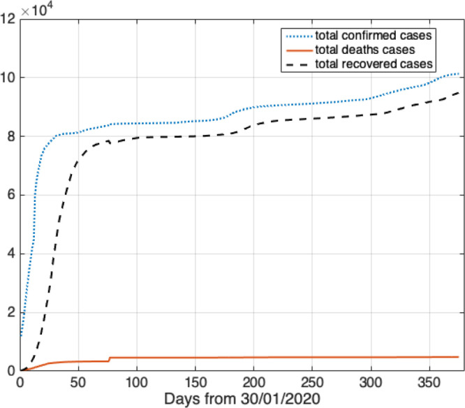
The total confirmed cases and recovered cases in China during the given time interval are shown in Fig. 2. On 31/01/2020, there were 11 821 cumulative confirmed cases in China. Then, the total confirmed cases were growing fast. On 29/02, there were 79 968 cumulative confirmed cases, which was 7 times higher than reported in the beginning of February. From 01/03, the growth of confirmed cases fell and became almost stable.

Fig. 2.

The pandemic trend of COVID-19 in China.

In Fig. 2, in the beginning of the outbreak, the high infection rate and the high low recovery rate are the characteristics of the period. In the March, the number of new confirmed cases flatten out. From 09/02, the number of recovered cases was growing fast.

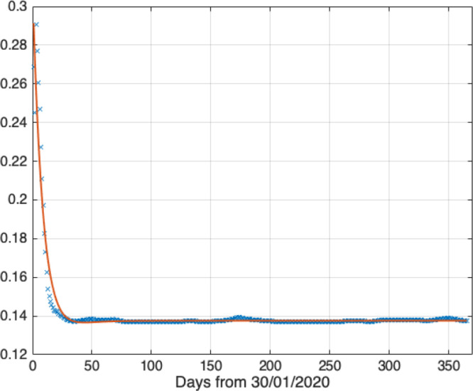
Before simulating the trend of COVID-19 in China, we should determine the function of the transmission probability. According to Eq. (14), the scatter diagram of $\beta \left(t\right)$ and the regression function during the time interval are shown in Fig. 3.

Fig. 3.

The scatter diagram of transmission probability and its regression function.

The regression function is shown as follows, and the R-square of this function is 0.9346:

$$\beta \left(t\right)=5.838\times exp(-0.09378\times t)-5.664\times exp(-0.09287\times t)+0.1376.$$ (25)

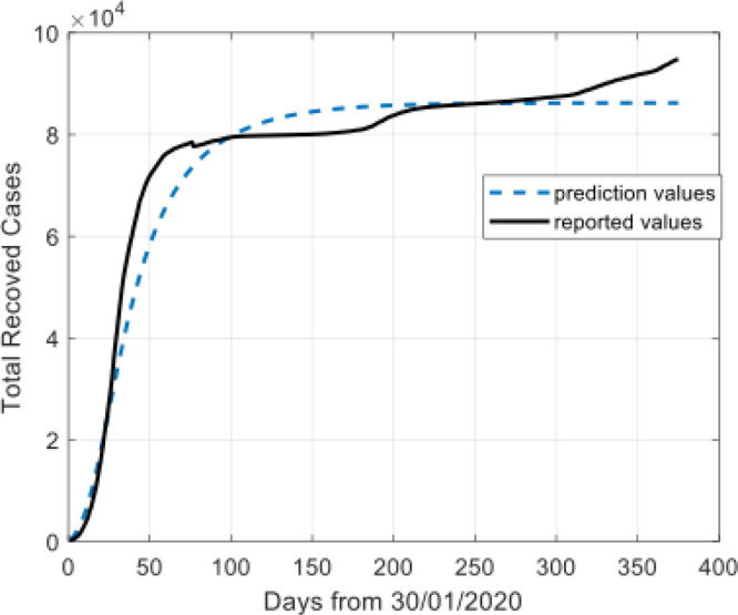
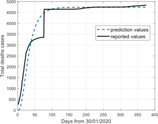
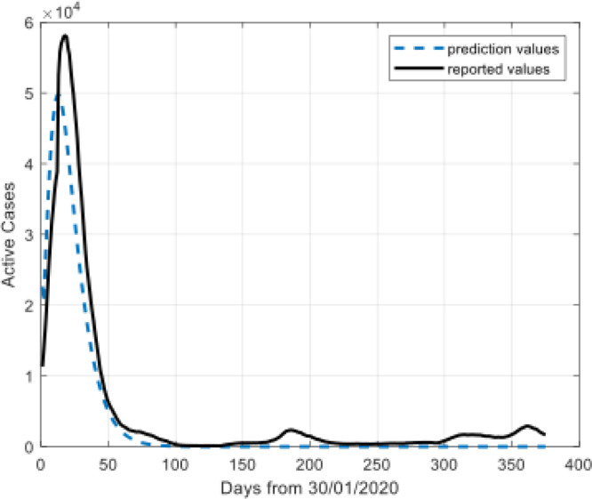
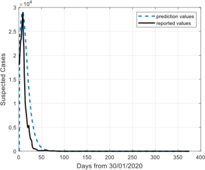
As shown in Fig. 3, the transmission probability was very large at the beginning of the outbreak, the transmission probability was reducing fast, and then flatten out. Taking the regression function into the Eq. (16) to simulate the pandemic trend of the disease, and then the model parameters can be estimated by comparison of the prediction values and the actual values. Fig. 4, Fig. 5, Fig. 6, Fig. 7 show the prediction results of the ISIR model for the recovered cases, the confirmed cases, the active cases, and the deaths cases in China.

Fig. 4.

Model results for total recovered cases.

Fig. 5.

Model results for total deaths cases.

Fig. 6.

Model results for active cases.

Fig. 7.

Model results for suspected cases.

The Fig. 4, Fig. 5, Fig. 6, Fig. 7 show that the prediction values demonstrate high similarity to the reported values. There is a remarkable fit between the actual number and the predicted cure in the time interval.

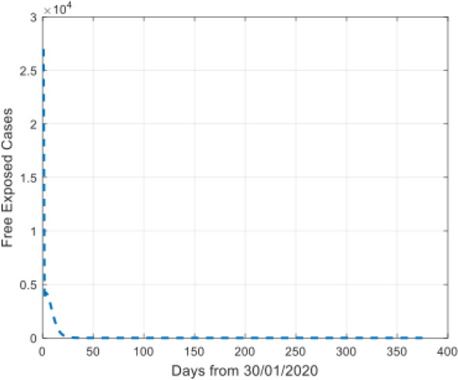
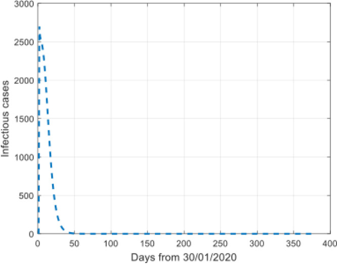
We also simulated the trend of the free exposed cases and the undiagnosed and non-isolated infectious individuals during the time interval, which were not reported on the website (see Fig. 8, Fig. 9).

Fig. 8.

Simulation of the free exposed cases.

Fig. 9.

Simulation of the infectious cases.

The Fig. 8, Fig. 9 show that the prediction values increase at the beginning of the disease and then reducing fast, and then flatten out.

The model parameters obtained from the inverse problem are listed as Table 1.

Table 1.

The estimated model parameters.

Parameter	Value
$ϵ$	0.26
$\alpha$	0.001
$d_{iq}$	0.004
$d_{ep}$	0.74
$d_{pq}$	0.14
$\gamma$	0.05

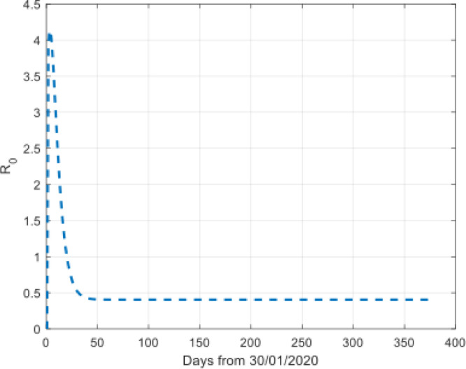
Taking these parameters into the Eq. (16), we can get the reproductive number of the disease as shown in Fig. 10.

Fig. 10.

The reproductive number during the time interval.

Fig. 10 indicates the disease had been under control. At the beginning of the outbreak, the reproductive number is very large. Then, It decreases to less than 0.5.

In a word, the ISIR model is proposed, which describes the pandemic trend of COVID-19 in China. We build the continuous model and discretize the model by forward-time finite-difference discretization. The nonlinear least squares inverse problem is constructed to estimate the unknown model parameters of ISIR. We simulate the trend of the disease under those model parameters. The numerical simulation results show that the prediction values demonstrate high similarity to the reported values. We also calculate the reproduction number of the disease, which is varied during the given time interval. It shows that the disease had been under the control in China.

CRediT authorship contribution statement

Wen-jing Zhu: Conceptualization, Methodology, Writing - original draft. Shou-feng Shen: Software, Writing - reviewing and editing.

Declaration of Competing Interest

The authors declare that they have no known competing financial interests or personal relationships that could have appeared to influence the work reported in this paper.

References

- 1.WHO, 2020. https://www.who.int/emergencies/diseases/novel-coronavirus-2019/ad-vice-for-public.
- 2.Worldometers, 2020. https://www.worldometers.info/coronavirus/.
- 3.Comunian Alessandro, Gaburro Romina, Giudici Mauro. Inversion of a SIR-based model: A critical analysis about the application to COVID-19 epidemic. Physica D. 2020;413 doi: 10.1016/j.physd.2020.132674. [DOI] [PMC free article] [PubMed] [Google Scholar]
- 4.Muoz-Fernndez Gustavo A., Seoane Jess M., Seoane-Seplveda Juan B. A SIR-type model describing the successive waves of COVID-19. Chaos Solitons Fractals. 2021;144 doi: 10.1016/j.chaos.2021.110682. [DOI] [PMC free article] [PubMed] [Google Scholar]
- 5.Umar Muhammad, Sabir Zulqurnain, Raja Muhammad Asif Zahoor, Snchez Yolanda Guerrero. A stochastic numerical computing heuristic of SIR nonlinear model based on dengue fever. Results Phys. 2020;19 [Google Scholar]
- 6.Rao V.S.H., Upadhyay R.K. Modeling the spread and outbreak dynamics of avian influenza (H5N1) virus and its possible control. In: Sree Hari Rao V., Durvasula R., editors. Dynamic models of infectious diseases. Springer; New York, NY: 2013. [Google Scholar]
- 7.Dhar M., Bhattacharya P. Analysis of SIR epidemic model with different basic reproduction numbers and validation with HIV and TSWV data. Iran J Sci Technol Trans Sci. 2019;43:2385–2397. [Google Scholar]
- 8.Ng T.W., Turinici G., Danchin A. A double epidemic model for the SARS propagation. BMC Infect Dis3. 2003;19 doi: 10.1186/1471-2334-3-19. [DOI] [PMC free article] [PubMed] [Google Scholar]
- 9.Cooper Ian, Mondal Argha, Antonopoulos Chris G. A SIR model assumption for the spread of COVID-19 in different communities. Chaos Solitons Fractals. 2020;139 doi: 10.1016/j.chaos.2020.110057. [DOI] [PMC free article] [PubMed] [Google Scholar]
- 10.Postnikov Eugene B. Estimation of COVID-19 dynamics on a back-of-envelope: Does the simplest SIR model provide quantitative parameters and predictions? Chaos Solitons Fractals. 2020;135 doi: 10.1016/j.chaos.2020.109841. [DOI] [PMC free article] [PubMed] [Google Scholar]
- 11.Kudryashov Nikolay A., Chmykhov Mikhail A., Vigdorowitsch Michael. Analytical features of the SIR model and their applications to COVID-19. Appl Math Model. 2021;90 doi: 10.1016/j.apm.2020.08.057. [DOI] [PMC free article] [PubMed] [Google Scholar]
- 12.Liu Xiaoping. A simple, SIR-like but individual-based epidemic model: Application in comparison of COVID-19 in New York City and Wuhan. Results Phys. 2021;20 doi: 10.1016/j.rinp.2020.103712. [DOI] [PMC free article] [PubMed] [Google Scholar]
- 13.Wang Peipei, Zheng Xinqi, Li Jiayang, Zhu Bangren. Prediction of epidemic trends in COVID-19 with logistic model and machine learning technics. Chaos Solitons Fractals. 2020;139 doi: 10.1016/j.chaos.2020.110058. [DOI] [PMC free article] [PubMed] [Google Scholar]
- 14.Malavika B., Marimuthu S., Joy Melvin, Nadaraj Ambily, Asirvatham Edwin Sam, Jeyaseelan L. Forecasting COVID-19 epidemic in India and high incidence states using SIR and logistic growth models. Clin Epidemiol Glob Health. 2021;9 doi: 10.1016/j.cegh.2020.06.006. [DOI] [PMC free article] [PubMed] [Google Scholar]
- 15.Abusam Abdallah, Abusam Razan, Al-Anzi Bader. Adequacy of logistic models for describing the dynamics of COVID-19 pandemic. Infec Dis Model. 2020;5 doi: 10.1016/j.idm.2020.08.006. [DOI] [PMC free article] [PubMed] [Google Scholar]
- 16.Shen Christopher Y. Logistic growth modelling of COVID-19 proliferation in China and its international implications. Int J Infec Dis. 2020;96 doi: 10.1016/j.ijid.2020.04.085. [DOI] [PMC free article] [PubMed] [Google Scholar]
- 17.Aviv-Sharon Elinor, Aharoni Asaph. Generalized logistic growth modeling of the COVID-19 pandemic in Asia. Infec Dis Model. 2020;5 doi: 10.1016/j.idm.2020.07.003. [DOI] [PMC free article] [PubMed] [Google Scholar]
- 18.Torrealba-Rodriguez O., Conde-Gutirrez R.A., Hernndez-Javier A.L. Modeling and prediction of COVID-19 in Mexico applying mathematical and computational models. Chaos Solitons Fractals. 2020;138 doi: 10.1016/j.chaos.2020.109946. [DOI] [PMC free article] [PubMed] [Google Scholar]
- 19.National Health Commission of the PRC, http://en.nhc.gov.cn.