A novel mathematical model for COVID-19 with remedial strategies

Abstract

Coronavirus (COVID-19) outbreak from Wuhan, Hubei province in China and spread out all over the World. In this work, a new mathematical model is proposed. The model consists the system of ODEs. The developed model describes the transmission pathways by employing non constant transmission rates with respect to the conditions of environment and epidemiology. There are many mathematical models purposed by many scientists. In this model, “${\alpha }_E$” and “${\alpha }_I$”, transmission coefficients of the exposed cases to susceptible and infectious cases to susceptible respectively, are included. “$\delta$” as a governmental action and restriction against the spread of coronavirus is also introduced. The RK method of order four (RK4) is employed to solve the model equations. The results are presented for four countries i.e., Pakistan, Italy, Japan, and Spain etc. The parametric study is also performed to validate the proposed model.

Introduction

Coronaviruses are a family of viruses responsible for respiratory diseases. At the end of 2019, a new type of coronavirus identified in Wuhan, China. The World Health Organization (WHO) gives a name to coronavirus as COVID-19. At the early stage 55% of first 425 confirmed cases were linked to the Huanan Seafood market [1], after this it spread from human to human. The disease novel coronavirus (COVID-19) started to spread in China and all over the World. It becomes a global concern in a few weeks. The WHO declared the novel coronavirus as a Global Public Health Emergency on 30^th January 2020 [2]. By 1^st March 2020, COVID-19 quickly spread in all the provinces of China and also it spread to 58 different countries [3], [4]. According to WHO at the end of March, there were 754,933 confirmed cases of COVID-19 and 36,522 deaths, on 31^th July 2020 there were 17,114,712 confirmed cases and 668,939 deaths in 216 countries or areas. Now on 30^th November 2020 there are 62,516,515 confirmed cases and 1,459,920 deaths in 220 countries or areas [5]. Currently, the outbreak of COVID-19 is ongoing and infection cases have been growing and deaths as well.

Modelling and simulations are very important decision tools that can be helpful to simulate and finally control epidemiological animal and human diseases[6], [7], [8]. However, every situation of disease exhibits it’s own particular biological behaviours and characteristics, the proposed models of diseases will be able to tackle the real situations. Coronavirus is a totally new virus and completely a new situation. COVID-19 gets the attention of scientists such as mathematicians who worked in mathematical modeling. In February and March 2020, some papers about this coronavirus were published [9], [10], [11], [12], [13]. Some investigations on spreading of novel coronavirus (COVID-19) in mainland China was useful to understand the outbreak of COVID-19 all over the world [14], [15], [16], [17], [18]. The paper [19] is based on three ODEs which is called the SIR model. There are many variants of the SEIR and SIR models found in the literature [20], [21], [22], [23], [24]. Many other models and solutions based on differential equations are presented in recent literature [25], [26], [27], [28], [29], [30]. Some of the authors also considered isolation and quarantine to reduce the spread of disease [31], [32], [33]. Similar studies were also reported in the literature for Turkey, Pakistan and South Africa [34], [35], [36]. Few recommendations are also provided by the researchers working in this area to reduce the effects of COVID-19 [37], [38], [39].

In this research, the effects of governmental action, weather conditions and individual reaction, except all other effects like new births and natural deaths, migration, etc are also included. Transmission rate from humans to humans are also included to make it a comprehensive study. SEIQR mathematical model (susceptible, exposed, infectious, quarantined, and removed) is proposed in this research, there exists a system of Ordinary Differential Equations. We also include isolation of peoples due to government action. In this model, we include “${\alpha }_E$”, as transmission coefficient of the exposed cases to susceptible and “${\alpha }_I$”, as transmission coefficient of the infectious cases to susceptible. Here we also introduce “$\delta$” as a governmental action and restriction against the spread of coronavirus. We conduct detailed analysis of model by using numerical methods as Runge Kutta method of order 4 (RK4) and Euler method, then manifest its applications by publicly reported data of different countries about coronavirus. In this research, proposed model is validated by considering four test problems. We use publicly available data about this virus to estimate the parameters. In these test problems, we provide complete overview about COVID-19 of Pakistan, Italy, Japan and Spain and also compare respectively the numerical result with the real reported data of virus of these mentioned countries. The results will be compared for above-mentioned countries on the base of governmental policies to control coronavirus, weather conditions, new cases, and deaths, etc.

The main motivation for this research is to explore the data of COVID-19 for four different countries with quantitative parameters. Safe and danger zones will also be highlighted after the detailed analysis of model and real data. Further more, quantitative analysis will help any health professional to predict the spread of pandemic as well as suggest how to control it by increasing safety measures to appropriate quantitative levels.

Model formulation

To model the coronavirus COVID-19, we proposed a new mathematical model, by introducing six different categories by dividing total human population in six compartments, i.e. $(S(t),E(t),I(t),Q(t),R(t),G(t))$ at time t the number of susceptible cases, exposed cases, infectious cases, quarantined cases, removed cases (recover and death both) and isolated cases (due to govt action).

The terms of developed model are defined as below:

Susceptible (S): Population of the region who is at risk of infection from disease.

Exposed (E): A person who may or may not infected from disease but not able to transmit.

Infectious (I): A person who is able to transmit the disease to other persons.

Quarantined (Q): A person who is under treatment and not able to meet other persons.

Removed (R): A person who got recovered or lost the life from disease.

Isolated (G): A person who is far away from other persons, objects, or society by government policy. Corresponding ODEs of model are given below:

$$\frac{\mathit{dS}(t)}{\mathit{dt}}=\mathrm{\Lambda }-{\alpha }_{E}S(t)E(t)-{\alpha }_{I}S(t)I(t)-\delta S(t)-\mu S(t),$$ (1)

$$\frac{\mathit{dE}(t)}{\mathit{dt}}={\alpha }_{E}S(t)E(t)+{\alpha }_{I}S(t)I(t)-\beta E(t)-\mu E(t),$$ (2)

$$\frac{\mathit{dI}(t)}{\mathit{dt}}=\beta E(t)-\gamma I(t)-\mu I(t),$$ (3)

$$\frac{\mathit{dQ}(t)}{\mathit{dt}}=\gamma I(t)-(r+d)Q(t)-\mu Q(t),$$ (4)

$$\frac{\mathit{dR}(t)}{\mathit{dt}}=(r+d)Q(t)-\mu R(t),$$ (5)

$$\frac{\mathit{dG}(t)}{\mathit{dt}}=\delta S(t)-\mu G(t)\text{.}$$ (6)

Here

$$S(0)={\phi }_1,E(0)={\phi }_2,I(0)={\phi }_3,Q(0)={\phi }_4,R(0)={\phi }_5,G(0)={\phi }_6,$$

and

$$\mathrm{\Lambda }=\omega N\text{.}$$

In this model “$\omega$” is birth rate, “${\alpha }_E$” is transmission rate from human to human, of the exposed cases to susceptible and “${\alpha }_I$” is also transmission rate from human to human, of the infectious cases to susceptible, “$\mu$” is natural death rate. The coefficients “${\beta }^{-1}$” and “${\gamma }^{-1}$ ” show the average latent time and average quarantine time(mean infectious period), “$\delta$” show protection rate, and “$r$” and “$d$” show cure rate and mortality rate. “$N$” represents total population. It is assumed that the recovered population will remain recovered throughout the process due to few reasons. The first reason is that COVID-19 recovered person will be more careful as compared to other population. Second reason is that due to variants of COVID-19 specially the p1 variant spread from Brazil is highly dangerous and people are more careful in general as compared to the previous waves of COVID-19. Third reason is that we do not have data available for such cases to support our model. Finally, not considering these negligible cases as susceptible, will make less complicated model.

Limitations:

• •No migration in or out.
• •Other external factors remain constant.
• •The vaccine of COVID-19 is not available.

$$S(t)+E(t)+I(t)+Q(t)+R(t)+G(t)=N,$$

Then followed by:

$$\frac{\mathit{dS}(t)}{\mathit{dt}}+\frac{\mathit{dE}(t)}{\mathit{dt}}+\frac{\mathit{dI}(t)}{\mathit{dt}}+\frac{\mathit{dQ}(t)}{\mathit{dt}}+\frac{\mathit{dR}(t)}{\mathit{dt}}+\frac{\mathit{dG}(t)}{\mathit{dt}}=0\text{.}$$

This model is solvable using different numerical schemes like Euler method and Runge Kutta method of different orders. In this study, Runge Kutta method of order 4 (RK4) is used to solve these differential equations.

The reproduction rate

In 1952, George Macdonald used $R_0$ first time in epidemiology to determine the spread of malaria. The reproduction ratio denoted by $R_0$, is important in the field of epidemiology. It is defined as “the average number of secondary infections produced when one infected individual is introduced into a population where everyone is susceptible ” [47]. Reproduction ratio is extremely useful because it helps us to determine whether the infection spreads through the population.

When the value of $R_0$ is less than 1, then infectious rate will be reduced and human population will remain healthy, while for the value of $R_0$ is greater than 1, the infection will spread in the population and it will be hard to control the epidemic.

Mathematical relation of $R_0$ is as follows:

$$R_0=\frac{(\beta {\alpha }_I+(\gamma +\mu ){\alpha }_E)}{\mu (\beta +\mu )(\gamma +\mu )}\text{.}$$

i $•$    If $R_0⩽1$ then Disease free equilibrium;

$$P_0=(\frac{\mathrm{\Lambda }}{\mu },0,0,0,0,0)\text{.}$$

ii $•$    If $R_0>1$, then, Disease will be present (Endemic Equilibrium);

$$P_1=(S,E,I,Q,R,G),$$

$$P_1(S,E,I,Q,R,G)>0\text{.}$$

Analysis of Model

In this section, the stability analysis is discussed by using linearizing method. Consider,

$$(S(t),E(t),I(t),Q(t),R(t),G(t))\in {\mathbb{R}}^6$$

. The feasible region $\mathrm{\Omega }$

$$\frac{\mathit{dN}}{\mathit{dt}}⩾0,$$

$$\begin{array}{c}\hfill \frac{\mathit{dN}}{\mathit{dt}}=\frac{d}{\mathit{dt}}\left(S(t)+E(t)+I(t)+Q(t)+R(t)+G(t)\right),\\ \hfill =\frac{\mathit{dS}(t)}{\mathit{dt}}+\frac{\mathit{dE}(t)}{\mathit{dt}}+\frac{\mathit{dI}(t)}{\mathit{dt}}+\frac{\mathit{dQ}(t)}{\mathit{dt}}+\frac{\mathit{dR}(t)}{\mathit{dt}}+\frac{\mathit{dG}(t)}{\mathit{dt}}\text{.}\end{array}$$

After putting the values, we have

$$\begin{array}{c}\hfill \frac{\mathit{dN}}{\mathit{dt}}=\mathrm{\Lambda }-\mu (S(t)+E(t)+I(t)+Q(t)+R(t)+G(t)),\\ \hfill =\mathrm{\Lambda }-\mu N⩾0\text{;}\frac{\mathrm{\Lambda }}{\mu }⩾N=S(t)+E(t)+I(t)+Q(t)+R(t)+G(t)\text{.}\\ \hfill \mathrm{\Omega }=\{S(t),E(t),I(t),Q(t),R(t),G(t))\in {\mathbb{R}}^6|S(t)+E(t)+I(t)+Q(t)+R(t)+G(t)⩽\frac{\mathrm{\Lambda }}{\mu }\}\text{.}\end{array}$$

Theorem

The system of Eqs. (1), (2), (3), (4), (5), (6) admits two equilibrium points $P_1=(1,0,0,0,0,0)$ and $P_2=(x_{10},x_{20},x_{30},x_{40},x_{50},x_{60})$, where $x_{10}=\frac{(\beta +\mu )(\gamma +\mu )}{\beta {\alpha }_I+(\gamma +\mu ){\alpha }_E},x_{20}=\frac{1}{(\beta +\mu )}\left[\mathrm{\Lambda }-\frac{(\delta +\mu )(\beta +\mu )(\gamma +\mu )}{\beta {\alpha }_I+(\gamma +\mu ){\alpha }_E}\right],x_{30}=\frac{\beta }{(\beta +\mu )(\gamma +\mu )}\left[\mathrm{\Lambda }-\frac{(\delta +\mu )(\beta +\mu )(\gamma +\mu )}{\beta {\alpha }_I+(\gamma +\mu ){\alpha }_E}\right],x_{40}=\frac{\beta \gamma }{(r+d+\mu )(\beta +\mu )(\gamma +\mu )}\left[\mathrm{\Lambda }-\frac{(\delta +\mu )(\beta +\mu )(\gamma +\mu )}{\beta {\alpha }_I+(\gamma +\mu ){\alpha }_E}\right]$,

$x_{50}=\frac{\beta \gamma (r+d)}{\mu (r+d+\mu )(\beta +\mu )(\gamma +\mu )}\left[\mathrm{\Lambda }-\frac{(\delta +\mu )(\beta +\mu )(\gamma +\mu )}{\beta {\alpha }_I+(\gamma +\mu ){\alpha }_E}\right],x_{60}=\frac{\delta }{\mu }\left[\frac{(\beta +\mu )(\gamma +\mu )}{\beta {\alpha }_I+(\gamma +\mu ){\alpha }_E}\right]$.

Proof:

The system of Eqs. (1), (2), (3), (4), (5), (6) is given as by replacing $S(t)\to x_1,E(t)\to x_2,I(t)\to x_3,Q(t)\to x_4,R(t)\to x_5,G(t)\to x_6$:

$$\frac{{\mathit{dx}}_1}{\mathit{dt}}=\mathrm{\Lambda }-{\alpha }_E{x}_1{x}_2-{\alpha }_I{x}_1{x}_3-\delta x_1-\mu x_1,$$ (7)

$$\frac{{\mathit{dx}}_2}{\mathit{dt}}={\alpha }_E{x}_1{x}_2+{\alpha }_I{x}_1{x}_3-\beta x_2-\mu x_2,$$ (8)

$$\frac{{\mathit{dx}}_3}{\mathit{dt}}=\beta x_2-\gamma x_3-\mu x_3,$$ (9)

$$\frac{{\mathit{dx}}_4}{\mathit{dt}}=\gamma x_3-(r+d)x_4-\mu x_4,$$ (10)

$$\frac{{\mathit{dx}}_5}{\mathit{dt}}=(r+d){\mathit{Qx}}_4-\mu x_5,$$ (11)

$$\frac{{\mathit{dx}}_6}{\mathit{dt}}=\delta x_1-\mu x_6\text{.}$$ (12)

The equilibrium points $(P_1\&P_2)$ satisfy the following relation:

$$\frac{{\mathit{dx}}_1}{\mathit{dt}}=\frac{{\mathit{dx}}_2}{\mathit{dt}}=\frac{{\mathit{dx}}_3}{\mathit{dt}}=\frac{{\mathit{dx}}_4}{\mathit{dt}}=\frac{{\mathit{dx}}_5}{\mathit{dt}}=\frac{{\mathit{dx}}_6}{\mathit{dt}}=0\text{.}$$ (13)

Putting Eqs. (7), (8), (9), (10), (11), (12) into Eq. 13, we get

$$\mathrm{\Lambda }-{\alpha }_E{x}_1{x}_2-{\alpha }_I{x}_1{x}_3-\delta x_1-\mu x_1=0,$$ (14)

$${\alpha }_E{x}_1{x}_2+{\alpha }_I{x}_1{x}_3-\beta x_2-\mu x_2=0,$$ (15)

$$\beta x_2-\gamma x_3-\mu x_3=0,$$ (16)

$$\gamma x_3-(r+d)x_4-\mu x_4=0,$$ (17)

$$(r+d){\mathit{Qx}}_4-\mu x_5=0,$$ (18)

$$\delta x_1-\mu x_6=0\text{.}$$ (19)

The first point $P_1=(1,0,0,0,0,0)$ is trivial in the sense that all the persons are healthy and stay healthy for all time. Now we find the second equilibrium point, for this we consider Eqs. (14), (15), (16), (17), (18), (19).

Adding Eqs. (14), (15), we obtain

$$\mathrm{\Lambda }-(\delta +\mu )x_1-(\beta +\mu )x_2=0,$$

$$x_2=\frac{\mathrm{\Lambda }-(\delta +\mu )x_1}{(\beta +\mu )}\text{.}$$ (20)

From Eq. 16, we have

$$x_3=\frac{\beta }{(\gamma +\mu )}{x}_2\text{.}$$ (21)

Putting the value $x_3$ into Eq. 15, we get

$${\alpha }_E{x}_1{x}_2+{\alpha }_I{x}_1(\frac{\beta }{(\gamma +\mu )}{x}_2)-\beta x_2-\mu x_2=0,$$

$${\alpha }_E{x}_1+{\alpha }_I{x}_1(\frac{\beta }{(\gamma +\mu )})-(\beta +\mu )=0,$$

$$x_1=\frac{(\beta +\mu )(\gamma +\mu )}{\beta {\alpha }_I+(\gamma +\mu ){\alpha }_E}\text{.}$$ (22)

Putting the value $x_1$ into Eq. 20, we obtain

$$x_2=\frac{1}{(\beta +\mu )}\left[\mathrm{\Lambda }-\frac{(\delta +\mu )(\beta +\mu )(\gamma +\mu )}{\beta {\alpha }_I+(\gamma +\mu ){\alpha }_E}\right]\text{.}$$ (23)

Putting the value $x_2$ into Eq. 21, we have

$$x_3=\frac{\beta }{(\beta +\mu )(\gamma +\mu )}\left[\mathrm{\Lambda }-\frac{(\delta +\mu )(\beta +\mu )(\gamma +\mu )}{\beta {\alpha }_I+(\gamma +\mu ){\alpha }_E}\right]\text{.}$$ (24)

From Eq. 17, we have

$$x_4=\frac{\gamma }{r+d+\mu }{x}_3,$$

putting the value $x_3$, we get

$$x_4=\frac{\beta \gamma }{(r+d+\mu )(\beta +\mu )(\gamma +\mu )}\left[\mathrm{\Lambda }-\frac{(\delta +\mu )(\beta +\mu )(\gamma +\mu )}{\beta {\alpha }_I+(\gamma +\mu ){\alpha }_E}\right]\text{.}$$ (25)

From Eq. 18, we have

$$x_5=\frac{r+d}{\mu }{x}_4,$$

putting the value $x_4$, we obtain

$$x_5=\frac{\beta \gamma (r+d)}{\mu (r+d+\mu )(\beta +\mu )(\gamma +\mu )}\left[\mathrm{\Lambda }-\frac{(\delta +\mu )(\beta +\mu )(\gamma +\mu )}{\beta {\alpha }_I+(\gamma +\mu ){\alpha }_E}\right]\text{.}$$ (26)

From Eq. 19, we have

$$x_6=\frac{\delta }{\mu }{x}_1,$$

putting the value $x_1$, we get

$$x_6=\frac{\delta }{\mu }\left[\frac{(\beta +\mu )(\gamma +\mu )}{\beta {\alpha }_I+(\gamma +\mu ){\alpha }_E}\right]\text{.}$$ (27)

The $P_2=(x_{10},x_{20},x_{30},x_{40},x_{50},x_{60})$ is the point that corresponds to the endemic state i.e. the COVID-19 disease persists in two population. The calculated values of $x_{10},x_{20},x_{30},x_{40},x_{50}$ and $x_{60}$ are given below:

$x_{10}=\frac{(\beta +\mu )(\gamma +\mu )}{\beta {\alpha }_I+(\gamma +\mu ){\alpha }_E},x_{20}=\frac{1}{(\beta +\mu )}\left[\mathrm{\Lambda }-\frac{(\delta +\mu )(\beta +\mu )(\gamma +\mu )}{\beta {\alpha }_I+(\gamma +\mu ){\alpha }_E}\right],x_{30}=\frac{\beta }{(\beta +\mu )(\gamma +\mu )}\left[\mathrm{\Lambda }-\frac{(\delta +\mu )(\beta +\mu )(\gamma +\mu )}{\beta {\alpha }_I+(\gamma +\mu ){\alpha }_E}\right],x_{40}=\frac{\beta \gamma }{(r+d+\mu )(\beta +\mu )(\gamma +\mu )}\left[\mathrm{\Lambda }-\frac{(\delta +\mu )(\beta +\mu )(\gamma +\mu )}{\beta {\alpha }_I+(\gamma +\mu ){\alpha }_E}\right],x_{50}=\frac{\beta \gamma (r+d)}{\mu (r+d+\mu )(\beta +\mu )(\gamma +\mu )}\left[\mathrm{\Lambda }-\frac{(\delta +\mu )(\beta +\mu )(\gamma +\mu )}{\beta {\alpha }_I+(\gamma +\mu ){\alpha }_E}\right],x_{60}=\frac{\delta }{\mu }\left[\frac{(\beta +\mu )(\gamma +\mu )}{\beta {\alpha }_I+(\gamma +\mu ){\alpha }_E}\right]$.

Hence it is proved that the system of Eqs. (1), (2), (3), (4), (5), (6) has two equilibrium $P_1=(1,0,0,0,0,0)$ and $P_2=(x_{10},x_{20},x_{30},x_{40},x_{50},x_{60})$ points.

Theorem

• 1. $•$      The equilibrium point at     $P_1=(1,0,0,0,0,0)$ is a saddle point.
• 2. $•$      The equilibrium point at     $P_2=(x_{10},x_{20},x_{30},x_{40},x_{50},x_{60})$ is asymptotically stable.

Here,       $x_{10}=\frac{(\beta +\mu )(\gamma +\mu )}{\beta {\alpha }_I+(\gamma +\mu ){\alpha }_E},x_{20}=\frac{1}{(\beta +\mu )}\left[\mathrm{\Lambda }-\frac{(\delta +\mu )(\beta +\mu )(\gamma +\mu )}{\beta {\alpha }_I+(\gamma +\mu ){\alpha }_E}\right],x_{30}=\frac{\beta }{(\beta +\mu )(\gamma +\mu )}\left[\mathrm{\Lambda }-\frac{(\delta +\mu )(\beta +\mu )(\gamma +\mu )}{\beta {\alpha }_I+(\gamma +\mu ){\alpha }_E}\right],x_{40}=\frac{\beta \gamma }{(r+d+\mu )(\beta +\mu )(\gamma +\mu )}\left[\mathrm{\Lambda }-\frac{(\delta +\mu )(\beta +\mu )(\gamma +\mu )}{\beta {\alpha }_I+(\gamma +\mu ){\alpha }_E}\right],x_{50}=\frac{\beta \gamma (r+d)}{\mu (r+d+\mu )(\beta +\mu )(\gamma +\mu )}\left[\mathrm{\Lambda }-\frac{(\delta +\mu )(\beta +\mu )(\gamma +\mu )}{\beta {\alpha }_I+(\gamma +\mu ){\alpha }_E}\right],x_{60}=\frac{\delta }{\mu }\left[\frac{(\beta +\mu )(\gamma +\mu )}{\beta {\alpha }_I+(\gamma +\mu ){\alpha }_E}\right]$.

Proof:

For simplicity, we let:

$$\frac{(\beta +\mu )(\gamma +\mu )}{\beta {\alpha }_I+(\gamma +\mu ){\alpha }_E}=\eta ,$$

$$\frac{1}{(\beta +\mu )}\left[\mathrm{\Lambda }-\frac{(\delta +\mu )(\beta +\mu )(\gamma +\mu )}{\beta {\alpha }_I+(\gamma +\mu ){\alpha }_E}\right]=\xi ,$$

and

$$\frac{\beta }{(\beta +\mu )(\gamma +\mu )}\left[\mathrm{\Lambda }-\frac{(\delta +\mu )(\beta +\mu )(\gamma +\mu )}{\beta {\alpha }_I+(\gamma +\mu ){\alpha }_E}\right]=\psi \text{.}$$

Then we have,

$x_{10}=\eta$,     $x_{20}=\xi$,     $x_{30}=\psi$,    $x_{40}=\frac{\gamma }{(r+d+\mu )}\left[\psi \right]$,     $x_{50}=\frac{\gamma (r+d)}{\mu (r+d+\mu )}\left[\psi \right]$,     $x_{60}=\frac{\delta }{\mu }\left[\eta \right]$.

The parameters values given in Table 1 . The values given in Table 1 are collected from WHO and calculated using statistical models [40], [41], [42], [43], [44], [45], [46].

Table 1.

Parameter values for Pakistan and Spain.

Name of parameter	Notation	Pakistan	Spain
Transmission rate of the exposed to susceptible	${\alpha }_E$	0.004253392	0.0261309
Transmission rate of the Infectious to susceptible	${\alpha }_I$	3.245065087	0.2619047
Protection rate	$\delta$	0.003505	0.0018373
Average latent time	${\beta }^{-1}$	0.0003551	0.0010819
Average quarantine	${\gamma }^{-1}$	0.1597073	0.1693473
Cure rate	r	0.058306850	0.1035586
Mortality rate	d	0.00414502	0.0156973
Birth Rate	$\omega$	27.530/1000	8.391/1000
Death rate	$\mu$	6.884/1000	9.200/1000

1 $•$    For finding the variational matrix, we use the system of model Eqs. (7), (12) at the first equilibrium point $P_1$, we get the following matrix.

$$\left(\begin{array}{cccccc}-(\delta +\mu )\hfill & -{\alpha }_E\hfill & -{\alpha }_I\hfill & 0\hfill & 0\hfill & 0\hfill \\ 0\hfill & {\alpha }_E-(\beta +\mu )\hfill & {\alpha }_I\hfill & 0\hfill & 0\hfill & 0\hfill \\ 0\hfill & \beta \hfill & -(\gamma +\mu )\hfill & 0\hfill & 0\hfill & 0\hfill \\ 0\hfill & 0\hfill & \gamma \hfill & -(r+d)-\mu \hfill & 0\hfill & 0\hfill \\ 0\hfill & 0\hfill & 0\hfill & (r+d)\hfill & -\mu \hfill & 0\hfill \\ \delta \hfill & 0\hfill & 0\hfill & 0\hfill & 0\hfill & -\mu \hfill \end{array}\right)$$ (28)

Using MAPLE for Eq. 28, the following characteristic equation is obtained.

${\lambda }^6+\left(6\mu +r+d+\gamma -{\alpha }_E+\beta +\delta \right){\lambda }^5+(\beta d+\beta \delta +\beta \gamma +5\beta \mu +\beta r-\beta {\alpha }_i+d\delta +d\gamma +5d\mu -d{\alpha }_E+\delta \gamma +5\delta \mu +\delta r-\delta {\alpha }_E+5\gamma \mu +\gamma r-\gamma {\alpha }_E+15{\mu }^2+5\mu r-5\mu {\alpha }_E-r{\alpha }_E){\lambda }^4$ $+(\beta d\delta +\beta d\gamma +4\beta d\mu -\beta d{\alpha }_i+\beta \delta \gamma +4\beta \delta \mu +\beta \delta r-\beta {\alpha }_i\delta +4\beta \gamma \mu +\beta \gamma r+10\beta {\mu }^2+4\beta \mu r-4\beta {\alpha }_i\mu -\beta r{\alpha }_i+d\delta \gamma +4d\delta \mu -d\delta {\alpha }_E+4d\gamma \mu -d\gamma {\alpha }_E+10d{\mu }^2-4d\mu {\alpha }_E+4\delta \gamma \mu +\delta \gamma r-\delta \gamma {\alpha }_E+10\delta {\mu }^2+4\delta \mu r-4\delta \mu {\alpha }_E-\delta r{\alpha }_E+10\gamma {\mu }^2+4\gamma \mu r-4\gamma \mu {\alpha }_E-\gamma r{\alpha }_E+20{\mu }^3+10{\mu }^{2}r-10{\mu }^2{\alpha }_E-4\mu r{\alpha }_E){\lambda }^3$ $+(\beta d\delta \gamma +3\beta d\delta \mu -\beta d\delta {\alpha }_i+3\beta d\gamma \mu +6\beta d{\mu }^2-3\beta d\mu {\alpha }_i+3\beta \delta \gamma \mu +\beta \delta \gamma r+6\beta \delta {\mu }^2+3\beta \delta \mu r-3\beta \delta \mu {\alpha }_i-\beta \delta r{\alpha }_i+6\beta \gamma {\mu }^2+3\beta \gamma \mu r+10\beta {\mu }^3+6\beta {\mu }^{2}r-6\beta {\mu }^2{\alpha }_i-3\beta \mu r{\alpha }_i+3d\delta \gamma \mu -d\delta \gamma {\alpha }_E+6d\delta {\mu }^2-3d\delta \mu {\alpha }_E+6d\gamma {\mu }^2-3d\gamma \mu {\alpha }_E+10d{\mu }^3-6d{\mu }^2{\alpha }_E+6\delta \gamma {\mu }^2+3\delta \gamma \mu r-3\delta \gamma \mu {\alpha }_E-\delta \gamma r{\alpha }_E+10\delta {\mu }^3+6\delta {\mu }^{2}r-6\delta {\mu }^2{\alpha }_E-3\delta \mu r{\alpha }_E+10\gamma {\mu }^3+6\gamma {\mu }^{2}r-6\gamma {\mu }^2{\alpha }_E-3\gamma \mu r{\alpha }_E+15{\mu }^4+10{\mu }^{3}r-10{\mu }^3{\alpha }_E-6{\mu }^{2}r{\alpha }_E){\lambda }^2$ $+(2\beta d\delta \gamma \mu +3\beta d\delta {\mu }^2-2\beta d\delta \mu {\alpha }_i+3\beta d\gamma {\mu }^2+4\beta d{\mu }^3-3\beta d{\mu }^2{\alpha }_i+3\beta \delta \gamma {\mu }^2+2\beta \delta \gamma \mu r+4\beta \delta {\mu }^3+3\beta \delta {\mu }^{2}r-3\beta \delta {\mu }^2{\alpha }_i-2\beta \delta \mu r{\alpha }_i+4\beta \gamma {\mu }^3+3\beta \gamma {\mu }^{2}r+5\beta {\mu }^4+4\beta {\mu }^{3}r-4\beta {\mu }^3{\alpha }_i-3\beta {\mu }^{2}r{\alpha }_i+3d\delta \gamma {\mu }^2-2d\delta \gamma \mu {\alpha }_E+4d\delta {\mu }^3-3d\delta {\mu }^2{\alpha }_E+4d\gamma {\mu }^3-3d\gamma {\mu }^2{\alpha }_E+5d{\mu }^4-4d{\mu }^3{\alpha }_E+4\delta \gamma {\mu }^3+3\delta \gamma {\mu }^{2}r-3\delta \gamma {\mu }^2{\alpha }_E-2\delta \gamma \mu r{\alpha }_E+5\delta {\mu }^4+4\delta {\mu }^{3}r-4\delta {\mu }^3{\alpha }_E-3\delta {\mu }^{2}r{\alpha }_E+5\gamma {\mu }^4+4\gamma {\mu }^{3}r-4\gamma {\mu }^3{\alpha }_E-3\gamma {\mu }^{2}r{\alpha }_E+6{\mu }^5+5{\mu }^{4}r-5{\mu }^4{\alpha }_E-4{\mu }^{3}r{\alpha }_E)\lambda +{\mu }^2\left(r+d+\mu \right)\beta \delta \gamma +\beta \delta \mu -\beta {\alpha }_i\delta +\beta \gamma \mu +\beta {\mu }^2-\beta {\alpha }_i\mu +\delta \gamma \mu -\delta \gamma {\alpha }_E+\delta {\mu }^2-\delta \mu {\alpha }_E+\gamma {\mu }^2-\gamma \mu {\alpha }_E+{\mu }^3-{\mu }^2{\alpha }_E)$.

Now we find the eigenvalues for the above equation at $P_1$ for Pakistan and Spain using Matlab.

The eigenvalues for Pakistan are as follows:

${\lambda }_1=-1.90508e^{-5}$,    ${\lambda }_2=-0.0355144028$,    ${\lambda }_3=-1.90508e^{-5}$,    ${\lambda }_4=-6.99028e-05e^{-5}$, 

${\lambda }_5=0.0116274950862875$,    ${\lambda }_6=-0.141096157344242$.

The eigenvalues for Spain are as follows:

${\lambda }_1=-2.54601e^{-5}$,     ${\lambda }_2=-0.1186935411$,     ${\lambda }_3=-2.54601e^{-5}$,     ${\lambda }_4=-0.0018627901$,  

${\lambda }_5=0.0265626422411319$,     ${\lambda }_6=-0.171187713904162$.

One eigenvalue at the first equilibrium point $P_1$ is positive in both Pakistan and Spain. Thus, $P_1$ is a saddle point, i.e over all population is healthy and is free of COVID-19 disease.

2 $•$    For finding the variational matrix we use the system of model Eqs. (7), (8), (9), (10), (11), (12) at the second equilibrium point $P_2$, we get the following matrix.

$$\left(\begin{array}{cccccc}-({\alpha }_E\xi +{\alpha }_I\psi +\delta +\mu )\hfill & -{\alpha }_E\eta \hfill & -{\alpha }_I\eta \hfill & 0\hfill & 0\hfill & 0\hfill \\ {\alpha }_E\xi +{\alpha }_I\psi \hfill & {\alpha }_E\eta -(\beta +\mu )\hfill & {\alpha }_I\eta \hfill & 0\hfill & 0\hfill & 0\hfill \\ 0\hfill & \beta \hfill & -(\gamma +\mu )\hfill & 0\hfill & 0\hfill & 0\hfill \\ 0\hfill & 0\hfill & \gamma \hfill & -(r+d)-\mu \hfill & 0\hfill & 0\hfill \\ 0\hfill & 0\hfill & 0\hfill & (r+d)\hfill & -\mu \hfill & 0\hfill \\ \delta \hfill & 0\hfill & 0\hfill & 0\hfill & 0\hfill & -\mu \hfill \end{array}\right)$$ (29)

Using MAPLE for Eq. 29, the following characteristic equation is obtained.

${\lambda }^6+({\alpha }_i\mathrm{\Psi }-{\alpha }_E\eta +{\alpha }_E\xi +\beta +d+\delta +\gamma +6\mu +r){\lambda }^5+(\mathrm{\Psi }\beta {\alpha }_i+\mathrm{\Psi }d{\alpha }_i+\mathrm{\Psi }\gamma {\alpha }_i+5\mathrm{\Psi }\mu {\alpha }_i+\mathrm{\Psi }r{\alpha }_i-\beta {\alpha }_i\eta +\beta \xi {\alpha }_E-d\eta {\alpha }_E+d\xi {\alpha }_E-\delta \eta {\alpha }_E-\gamma \eta {\alpha }_E-5\eta \mu {\alpha }_E-\eta r{\alpha }_E+\gamma \xi {\alpha }_E+5\mu \xi {\alpha }_E+r\xi {\alpha }_E+d\beta +\beta \delta +\gamma \beta +5\beta \mu +r\beta +d\delta +d\gamma +5d\mu +\gamma \delta +5\mu \delta +r\delta +5\gamma \mu +r\gamma +15{\mu }^2+5r\mu ){\lambda }^4$ $+(\mathrm{\Psi }\beta d{\alpha }_i+\mathrm{\Psi }\beta \gamma {\alpha }_i+4\mathrm{\Psi }\beta \mu {\alpha }_i+\mathrm{\Psi }\beta r{\alpha }_i+\mathrm{\Psi }d\gamma {\alpha }_i+4\mathrm{\Psi }d\mu {\alpha }_i+4\mathrm{\Psi }\gamma \mu {\alpha }_i+\mathrm{\Psi }\gamma r{\alpha }_i+10\mathrm{\Psi }{\mu }^2{\alpha }_i+4\mathrm{\Psi }\mu r{\alpha }_i-\beta d\eta {\alpha }_i+\beta d\xi {\alpha }_E-\beta \delta \eta {\alpha }_i-4\beta \eta \mu {\alpha }_i-\beta \eta r{\alpha }_i+\beta \gamma \xi {\alpha }_E+4\beta \mu \xi {\alpha }_E+\beta r\xi {\alpha }_E-d\delta \eta {\alpha }_E-\gamma d\eta {\alpha }_E-4d\eta \mu {\alpha }_E+d\gamma \xi {\alpha }_E+4d\mu \xi {\alpha }_E-\gamma \delta \eta {\alpha }_E-4\delta \eta \mu {\alpha }_E-\delta \eta r{\alpha }_E-4\gamma \eta \mu {\alpha }_E-\gamma \eta r{\alpha }_E-10\eta {\mu }^2{\alpha }_E-4\eta \mu r{\alpha }_E+4\gamma \mu \xi {\alpha }_E+\gamma r\xi {\alpha }_E+10{\mu }^2\xi {\alpha }_E+4\mu r\xi {\alpha }_E+\beta d\delta +\gamma \beta d+4\beta d\mu +\gamma \beta \delta +4\beta \delta \mu +\beta \delta r+4\gamma \beta \mu +\gamma \beta r+10\beta {\mu }^2+4\beta \mu r+\gamma d\delta +4d\delta \mu +4\gamma d\mu +10d{\mu }^2+4\gamma \delta \mu +\gamma \delta r+10\delta {\mu }^2+4\delta \mu r+10\gamma {\mu }^2+4\gamma \mu r+20{\mu }^3+10{\mu }^{2}r){\lambda }^3$ $+(\mathrm{\Psi }\beta d\gamma {\alpha }_i+3\mathrm{\Psi }\beta d\mu {\alpha }_i+3\mathrm{\Psi }\beta \gamma \mu {\alpha }_i+\mathrm{\Psi }\beta \gamma r{\alpha }_i+6\mathrm{\Psi }\beta {\mu }^2{\alpha }_i+3\mathrm{\Psi }\beta \mu r{\alpha }_i+3\mathrm{\Psi }d\gamma \mu {\alpha }_i+6\mathrm{\Psi }d{\mu }^2{\alpha }_i+6\mathrm{\Psi }\gamma {\mu }^2{\alpha }_i+3\mathrm{\Psi }\gamma \mu r{\alpha }_i+10\mathrm{\Psi }{\mu }^3{\alpha }_i+6\mathrm{\Psi }{\mu }^{2}r{\alpha }_i-\beta d\delta \eta {\alpha }_i-3\beta d\eta \mu {\alpha }_i+\beta d\gamma \xi {\alpha }_E+3\beta d\mu \xi {\alpha }_E-3\beta \delta \eta \mu {\alpha }_i-\beta \delta \eta r{\alpha }_i-6\beta \eta {\mu }^2{\alpha }_i-3\beta \eta \mu r{\alpha }_i+3\beta \gamma \mu \xi {\alpha }_E+\beta \gamma r\xi {\alpha }_E+6\beta {\mu }^2\xi {\alpha }_E+3\beta \mu r\xi {\alpha }_E-\gamma d\delta \eta {\alpha }_E-3d\delta \eta \mu {\alpha }_E-3\gamma d\eta \mu {\alpha }_E-6d\eta {\mu }^2{\alpha }_E+3d\gamma \mu \xi {\alpha }_E+6d{\mu }^2\xi {\alpha }_E-3\gamma \delta \eta \mu {\alpha }_E-\gamma \delta \eta r{\alpha }_E-6\delta \eta {\mu }^2{\alpha }_E-3\delta \eta \mu r{\alpha }_E-6\gamma \eta {\mu }^2{\alpha }_E-3\gamma \eta \mu r{\alpha }_E-10\eta {\mu }^3{\alpha }_E-6\eta {\mu }^{2}r{\alpha }_E+6\gamma {\mu }^2\xi {\alpha }_E+3\gamma \mu r\xi {\alpha }_E+10{\mu }^3\xi {\alpha }_E+6{\mu }^{2}r\xi {\alpha }_E+\gamma \beta d\delta +3\beta d\delta \mu +3\gamma \beta d\mu +6\beta d{\mu }^2+3\gamma \beta \delta \mu +\gamma \beta \delta r+6\beta \delta {\mu }^2+3\beta \delta \mu r+6\gamma \beta {\mu }^2+3\gamma \beta \mu r+10\beta {\mu }^3+6\beta {\mu }^{2}r+3\gamma d\delta \mu +6d\delta {\mu }^2+6\gamma d{\mu }^2+10d{\mu }^3+6\gamma \delta {\mu }^2+3\gamma \delta \mu r+10\delta {\mu }^3+6\delta {\mu }^{2}r+10\gamma {\mu }^3+6\gamma {\mu }^{2}r+15{\mu }^4+10{\mu }^{3}r){\lambda }^2$ $+(2\mathrm{\Psi }\beta d\gamma \mu {\alpha }_i+3\mathrm{\Psi }\beta d{\mu }^2{\alpha }_i+3\mathrm{\Psi }\beta \gamma {\mu }^2{\alpha }_i+2\mathrm{\Psi }\beta \gamma \mu r{\alpha }_i+4\mathrm{\Psi }\beta {\mu }^3{\alpha }_i+3\mathrm{\Psi }\beta {\mu }^{2}r{\alpha }_i+3\mathrm{\Psi }d\gamma {\mu }^2{\alpha }_i+4\mathrm{\Psi }d{\mu }^3{\alpha }_i+4\mathrm{\Psi }\gamma {\mu }^3{\alpha }_i+3\mathrm{\Psi }\gamma {\mu }^{2}r{\alpha }_i+5\mathrm{\Psi }{\mu }^4{\alpha }_i+4\mathrm{\Psi }{\mu }^{3}r{\alpha }_i-2\beta d\delta \eta \mu {\alpha }_i-3\beta d\eta {\mu }^2{\alpha }_i+2\beta d\gamma \mu \xi {\alpha }_E+3\beta d{\mu }^2\xi {\alpha }_E-3\beta \delta \eta {\mu }^2{\alpha }_i-2\beta \delta \eta \mu r{\alpha }_i-4\beta \eta {\mu }^3{\alpha }_i-3\beta \eta {\mu }^{2}r{\alpha }_i+3\beta \gamma {\mu }^2\xi {\alpha }_E+2\beta \gamma \mu r\xi {\alpha }_E+4\beta {\mu }^3\xi {\alpha }_E+3\beta {\mu }^{2}r\xi {\alpha }_E-2\gamma d\delta \eta \mu {\alpha }_E-3d\delta \eta {\mu }^2{\alpha }_E-3\gamma d\eta {\mu }^2{\alpha }_E-4d\eta {\mu }^3{\alpha }_E+3d\gamma {\mu }^2\xi {\alpha }_E+4d{\mu }^3\xi {\alpha }_E-3\gamma \delta \eta {\mu }^2{\alpha }_E-2\gamma \delta \eta \mu r{\alpha }_E-4\delta \eta {\mu }^3{\alpha }_E-3\delta \eta {\mu }^{2}r{\alpha }_E-4\gamma \eta {\mu }^3{\alpha }_E-3\gamma \eta {\mu }^{2}r{\alpha }_E-5\eta {\mu }^4{\alpha }_E-4\eta {\mu }^{3}r{\alpha }_E+4\gamma {\mu }^3\xi {\alpha }_E+3\gamma {\mu }^{2}r\xi {\alpha }_E+5{\mu }^4\xi {\alpha }_E+4{\mu }^{3}r\xi {\alpha }_E+2\gamma \beta d\delta \mu +3\beta d\delta {\mu }^2+3\gamma \beta d{\mu }^2+4\beta d{\mu }^3+3\gamma \beta \delta {\mu }^2+2\gamma \beta \delta \mu r+4\beta \delta {\mu }^3+3\beta \delta {\mu }^{2}r+4\gamma \beta {\mu }^3+3\gamma \beta {\mu }^{2}r+5\beta {\mu }^4+4\beta {\mu }^{3}r+3\gamma d\delta {\mu }^2+4d\delta {\mu }^3+4\gamma d{\mu }^3+5d{\mu }^4+4\gamma \delta {\mu }^3+3\gamma \delta {\mu }^{2}r+5\delta {\mu }^4+4\delta {\mu }^{3}r+5\gamma {\mu }^4+4\gamma {\mu }^{3}r+6{\mu }^5+5{\mu }^{4}r)\lambda$ $+{\mu }^2(r+d+\mu )(\mathrm{\Psi }\beta \gamma {\alpha }_i+\mathrm{\Psi }\beta \mu {\alpha }_i+\mathrm{\Psi }\gamma \mu {\alpha }_i+\mathrm{\Psi }{\mu }^2{\alpha }_i-\beta \delta \eta {\alpha }_i-\beta \eta \mu {\alpha }_i+\beta \gamma \xi {\alpha }_E+\beta \mu \xi {\alpha }_E-\gamma \delta \eta {\alpha }_E-\delta \eta \mu {\alpha }_E-\gamma \eta \mu {\alpha }_E-\eta {\mu }^2{\alpha }_E+\gamma \mu \xi {\alpha }_E+{\mu }^2\xi {\alpha }_E+\gamma \beta \delta +\beta \delta \mu +\gamma \beta \mu +\beta {\mu }^2+\gamma \delta \mu +\delta {\mu }^2+\gamma {\mu }^2+{\mu }^3)$.

Now we find the eigenvalues using MATLAB from the above equation for Pakistan and Spain.

The eigenvalues for Pakistan are as follows:

${\lambda }_1=-1.90508e^{-5}$,    ${\lambda }_2=-0.0355144028$,    ${\lambda }_3=-1.90508e^{-5}$,    ${\lambda }_4=-5.08220963929699e^5$, 

${\lambda }_5=-0.000394150800098247$,    ${\lambda }_6=-0.1410769508$.

The eigenvalues for Spain are as follows:

${\lambda }_1=-2.54601e^{-5}$,     ${\lambda }_2=-0.1186935411$,     ${\lambda }_3=-2.54601e^{-5}$,     ${\lambda }_4=-21955.2092485067$,  

${\lambda }_5=-0.00138325809703833$,     ${\lambda }_6=-0.169372760014153$.

All the eigenvalues are negative at $P_2$, thus the point $P_2$ is asymptotically stable for both Pakistan and Spain. The population will have COVID-19 disease.

Positivity of Solution

The modelling of COVID-19 will be meaningful, if the solution of the system are non-negative initial condition will remain positive for all $t>0$ .

Theorem

For all $t>0$ and initial conditions $P(0)⩾0$ where $P(t)=(S,E,I,Q,R,G)$ the solution of the model are positive for all $t>0$.

Proof:

Consider Eq. 1 of the COVID-19 model,

$$\frac{\mathit{dS}(t)}{\mathit{dt}}=\mathrm{\Lambda }-{\alpha }_{E}S(t)E(t)-{\alpha }_{I}S(t)I(t)-\delta S(t)-\mu S(t)$$

$$\frac{\mathit{dS}(t)}{\mathit{dt}}=-({\alpha }_{E}E(t)+{\alpha }_{I}I(t)+\mu )S(t)-\delta S(t)+\mathrm{\Lambda }$$

Now we let ${\lambda }_1(t)=({\alpha }_{E}E(t)+{\alpha }_{I}I(t)+\mu )$ and ${\lambda }_2(t)=\mathrm{\Lambda }$, then above equation become,

$$\frac{\mathit{dS}(t)}{\mathit{dt}}=-({\lambda }_1(t))S(t)-\delta S(t)+{\lambda }_2(t)$$

$$\frac{\mathit{dS}(t)}{\mathit{dt}}=-({\lambda }_1(t)+\delta )S(t)+{\lambda }_2(t)$$ (30)

Taking integration on both sides of Eq. (30),

$$\frac{d}{\mathit{dt}}\left[S(t)\exp \left\{\mathit{dt}+{\int }_0^t{\lambda }_2(S)\mathit{dS}\right\}\right]={\lambda }_2(t)\exp \left\{\delta t+{\int }_0^t{\lambda }_1(S)\mathit{dS}\right\}$$

Hence

$$\left[S(t)\exp \left\{\mathit{dt}+{\int }_0^{t_1}{\lambda }_2(S)\mathit{dS}\right\}-S(0)\right]={\int }_0^{t_1}{\lambda }_2(t)\exp \left\{\delta S+{\int }_0^S{\lambda }_1(S)\mathit{dS}\right\}\mathit{dS}$$

Thus the solution of the above equation is

$$S(t_1)=S(0)\exp \left\{-\left(d(t_1)+{\int }_0^{t_1}{\lambda }_2(S)\mathit{dS}\right)\right\}+\exp \left\{-\left(d(t_1)+{\int }_0^{t_1}{\lambda }_2(S)\mathit{dS}\right)\right\}$$

$$\times {\int }_0^{t_1}{\lambda }_2(t)\exp \left\{\delta S+{\int }_0^S{\lambda }_1(S)\mathit{dS}\right\}\mathit{dS}>0$$

Similarly it can be shown that the quantities (E, I, Q, R, G) are positive for $P>0$ and for all time $t>0$.

Numerical test problems

The mathematical model is applied to study the first and the second wave of epidemic COVID-19 in different countries such as Pakistan, Italy, Japan and Spain. The second wave is stronger than first wave of COVID-19. We use the outbreak data daily published by World Health Organization (WHO) and other sources [40], [41], [42], [43], [44], [45], [46]. The collected data sets consist of susceptible population, exposed and infectious cases, new reported quarantined cases, recovered cases and deaths due to COVID-19 of above mentioned countries. The RK4 is employed to solve the model equations.

Algorithm

Suppose we have m differential equations:

$$\begin{array}{c}\hfill y_1^{\prime }=g_1(t,y_1,y_2,\dots ,y_m)\\ \hfill y_2^{\prime }=g_2(t,y_1,y_2,\dots ,y_m)\\ \hfill .\text{.}\\ \hfill .\text{.}\\ \hfill y_m^{\prime }=g_m(t,y_1,y_2,\dots ,y_m),\end{array}$$

with the initial conditions,

$$y_1(t_0)=y_{10},y_2(t_0)=y_{20},\dots ,y_m(t_0)=y_{m0}\text{.}$$

There is no derivative on the right hand side and all of these m equations are of order one. RK4 formula is as follows:

$$y_{i,n+1}=y_{i,n}+\frac{h}{6}(L_{i,1}+2L_{i,2}+2L_{i,3}+L_{i,4}),$$ (31)

$$t_{n+1}=t_n+h,$$ (32)

where,

$$L_{i,1}=g_i(t_n,y_{1n},y_{2n},...,y_{\mathit{mn}}),$$ (33)

$$L_{i,2}=g_i(t_n+\frac{h}{2},y_{1n}+\frac{h}{2}{L}_{11},y_{2n}+\frac{h}{2}{L}_{21},\dots ,y_{\mathit{mn}}+\frac{h}{2}{L}_{m1}),$$ (34)

$$L_{i,3}=g_i(t_n+\frac{h}{2},y_{1n}+\frac{h}{2}{L}_{12},y_{2n}+\frac{h}{2}{L}_{22},\dots ,y_{\mathit{mn}}+\frac{h}{2}{L}_{m2}),$$ (35)

$$L_{i,4}=g_i(t_n+h,y_{1n}+{\mathit{hL}}_{13},y_{2n}+{\mathit{hL}}_{23},...,y_{\mathit{mn}}+{\mathit{hL}}_{m3})\text{.}$$ (36)

where $y_{i,n+1}$ is the RK4 approximation of $y(t_{i,n+1})$ and h is step size.

For numerical simulation, we consider four test problems and their comparisons with each other.

• 1.Test problem 1: Pakistan
• 2.Test problem 2: Italy
• 3.Test problem 3: Japan
• 4.Test problem 4: Spain

Test Problem 1: Pakistan

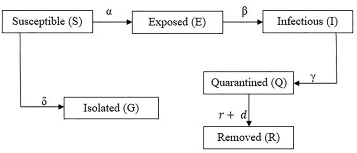
In Pakistan, COVID-19 spread out mostly from China and Iran. In start four Pakistani students in China effected from coronavirus. After this, many students and other people came back from China, Iran and other countries with positive tests of coronavirus. They came back to home and met with other people, in this way, coronavirus started to spread in all over Pakistan. Due to high risk of COVID-19, government took actions to control international traffics and bound all the people in their homes. One time Government successfully controlled coronavirus and step wise took off lock-down but from end of October second wave of coronavirus started in Pakistan and all over the World. During first coronavirus wave from 15th March, 2020 to 31st August, 2020, Pakistan faces 2,95,849 positive cases, 97.8% people recovered and 2.2% people died. Up to 30th November, there were total 4,00,482 positive cases, at the same time 97.7% people recovered from coronavirus and 2.3% people died due to coronavirus. Fig. 1 shows the proposed model of COVID-19 with inclusion of government policy.

Fig. 1.

Proposed Model of COVID-19 with inclusion of government policy.

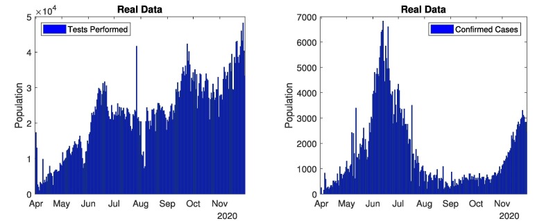
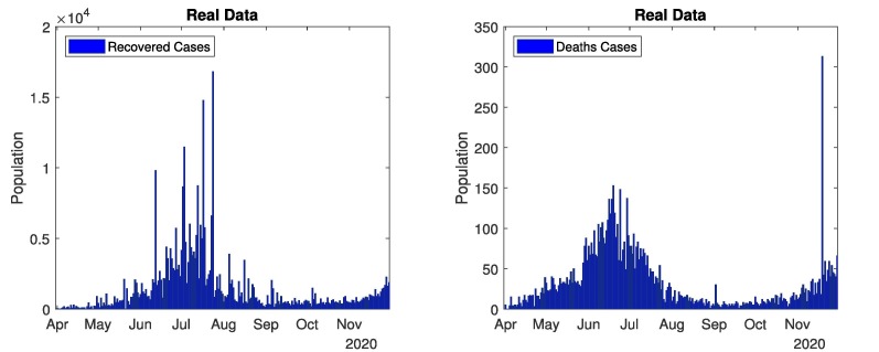
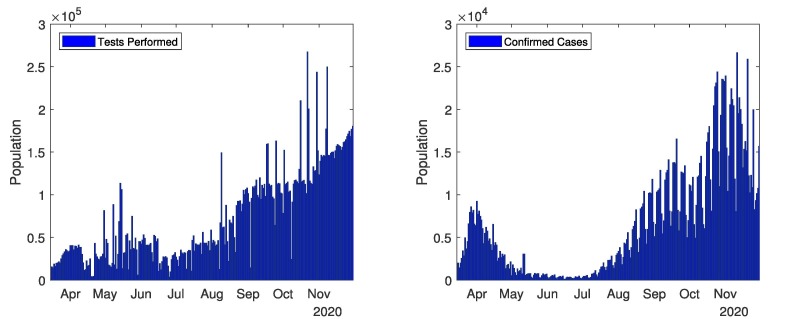
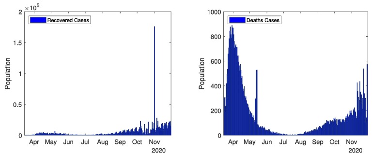
The current and complete overview of COVID-19 in all over Pakistan shown in Fig. 2, Fig. 3 . These Figures represents the real data of tests performed, confirmed cases, deaths cases and recovered cases. Data related to COVID-19 cases of Pakistan are taken from different sources [40], [41], [43]. Fig. 2 (first graph) depicts the number of tests performed from 1st April, 2020 to 30th November, 2020. Mostly tests are performed in September (highest 42,299 in one day and total 8,93,091 in a month). The total tests performed till 30th November, 2020 are 55,08,810. Fig. 2 (second graph) represents the confirmed cases from 1st April, 2020 to 30th November, 2020. Coronavirus started from 15th March in Pakistan, and continuously increased till mid of June, and then decreased till September. There were most confirmed cases in June (highest 6,825 in one day and total 1,41,010 in a month). The total confirmed cases in Pakistan are 4,00,482 till 30th November, 2020. The confirmed cases are still increasing. The government closed all the public points, implemented a strict lockdown and aware the masses to follows the SOPs. Due to government polices, the COVID-19 remained in control from end of June to mid of October. In October, the government took off the lockdown and coronavirus spread again. Fig. 3 (first graph) represents recovered cases from 1st April, 2020 to 30th November, 2020. In total 3,43,282 recovered people till 30th November, 2020. Fig. 3 (second graph) represents the number of deaths from 1st April to 30th November, 2020. As most cases were observed in June and July thus most deaths occurred in June and July. In total 8,091 deaths till 30th November, 2020.

Fig. 2.

In Pakistan: Tests performed and confirmed cases.

Fig. 3.

In Pakistan: Recovered cases and deaths Cases.

The model given in Eqs. (1), (2), (3), (4), (5), (6) are solved using RK4. The simulated results of model equations (c.f Eqs. (1), (2), (3), (4), (5), (6)) are presented. For the estimation of the values of parameters, the statistics terminologies are used. The parameters values are given in Table 1. The comparison of simulated results and real data of infectious and removed cases are provided in graphs.

Problem   1:

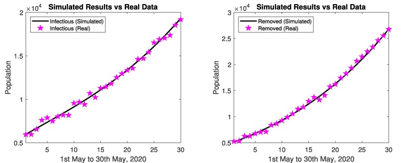
The comparison of simulated results and real data, during 1st coronavirus wave presented below. Fig. 4 represents comparison of simulated results and real data of infectious and removed cases from 1st May, 2020 to 30 May, 2020. The simulated results are close to the real data in infectious and removed cases as depicted in Fig. 4.

Fig. 4.

In Pakistan: Simulated results and real data of May 2020.

Problem   2:

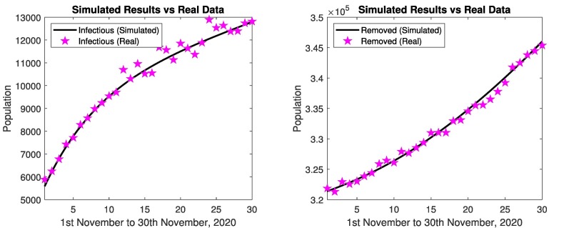
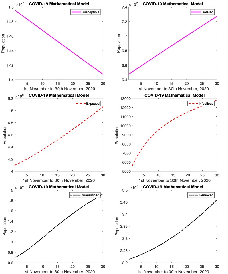
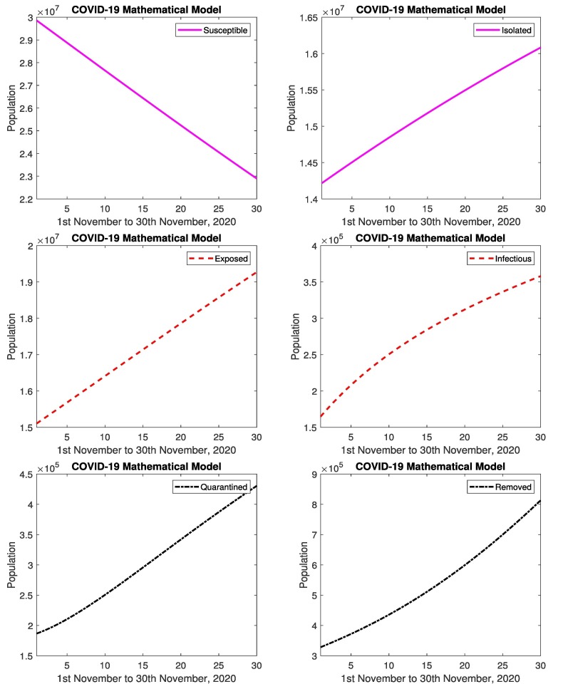
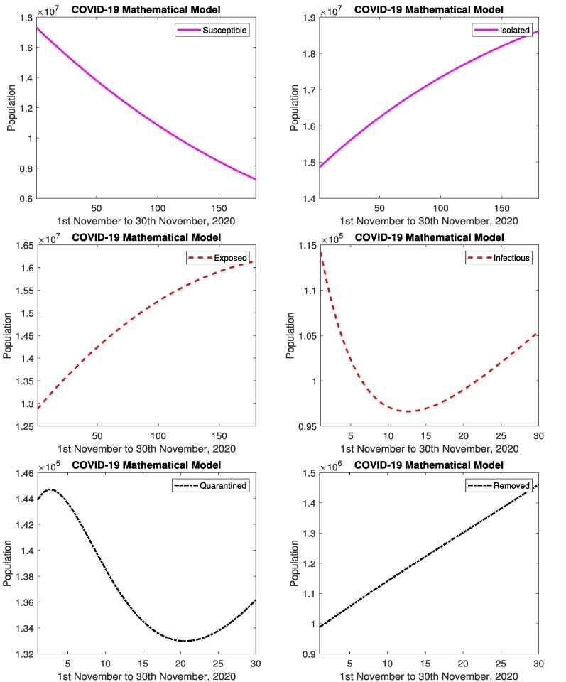
In Fig. 5 represents the simulated results and real data of infectious and removed cases from 1st November to 30th November, 2020. The simulated results are close to the real data in infectious and removed cases, relative errors are given in the Table 2, Table 3 . Figs. 6 represents the simulated results of the model (susceptible, isolated, exposed, infectious, quarantined and removed cases) from 1st November to 30th November, 2020. The results shows the decrease in susceptible population and increase in infected and removed population. Similarly the exposed cases and isolated cases increases. The affected people are recovering from disease. When the people follow the SOPs, then decrease in infectious and quarantined cases, and increase in isolation. When the government strictly implements the SOP’s against the spread of coronavirus then isolated population increase rapidly.

Fig. 5.

In Pakistan: Simulated results and real data of November 2020.

Table 2.

Study of relative errors of infectious cases for Pakistan.

Date	Relative errors	Date	Relative errors	Date	Relative errors
1st Nov	0.00353714	11th Nov	0.018611967	21st Nov	0.022530718
2nd Nov	0.059333762	12th Nov	0.04961982	22nd Nov	0.014370193
3rd Nov	0.016483681	13th Nov	0.03904853	23rd Nov	0.017295136
4th Nov	0.077882919	14th Nov	0.043724446	24th Nov	0.004993105
5th Nov	0.066274092	15th Nov	0.016915839	25th Nov	0.026576735
6th Nov	0.02744429	16th Nov	0.006657531	26th Nov	0.012788158
7th Nov	0.004037946	17th Nov	0.012635892	27th Nov	0.015288762
8th Nov	0.026160779	18th Nov	0.008455499	28th Nov	0.03361372
9th Nov	0.072072323	19th Nov	0.005058541	29th Nov	0.004347435
10th Nov	0.044731812	20th Nov	0.002280837	30th Nov	0.006717684

Table 3.

Study of relative errors of removed cases for Pakistan.

Date	Relative errors	Date	Relative errors	Date	Relative errors
1st Nov	0.022848439	11th Nov	0.001014855	21st Nov	0.014829661
2nd Nov	0.03479109	12th Nov	0.007550067	22nd Nov	0.010417078
3rd Nov	0.055548059	13th Nov	0.032253553	23rd Nov	0.015949148
4th Nov	0.013282583	14th Nov	0.006472368	24th Nov	0.031151726
5th Nov	0.005404622	15th Nov	0.040744057	25th Nov	0.02244561
6th Nov	0.030001821	16th Nov	0.041790411	26th Nov	0.017771562
7th Nov	0.083562877	17th Nov	0.050551446	27th Nov	0.007295753
8th Nov	0.018183534	18th Nov	0.040348327	28th Nov	0.011238798
9th Nov	0.009819484	19th Nov	0.018725169	29th Nov	0.000512259
10th Nov	0.003797866	20th Nov	0.004873214	30th Nov	0.000952095

Fig. 6.

In Pakistan: Simulated results of susceptible, isolated, exposed, infectious, quarantined and removed cases from 1st November to 30th November, 2020.

Table 2 represents the relative errors from 1st November to 30th November, 2020 of infectious cases. We see that the relative errors are less than 1 for all days. Table 3 represents relative errors from 1st November to 30th November, 2020 of removed cases. We see that the relative errors are less than 1 for all days, which verify the correctness of model formulation. The developed mathematical model can be helpful to measure the coronavirus situations.

Problem   3: Prediction for Next 6 Months

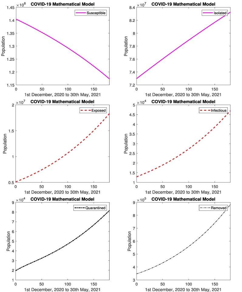
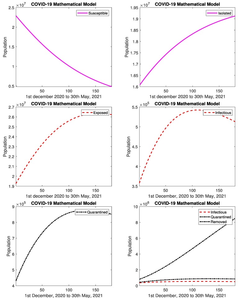
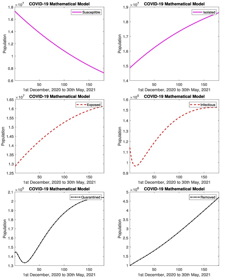
The prediction of COVID-19 using the mathematical model is presented. Fig. 7 represents the prediction of COVID-19 for 180 days. The simulated results by developed model of COVID-19 (1st December, 2020 to 30th May, 2021) are presented. The results show that the number of infected cases are increasing almost 265%. As the infected increases, the suspected decreases 16%, which is clearly depicted in Fig. 7. Fig. 7 depicts that number of removed cases are increasing. According to the results, the infected population due to COVID-19 will increase and the educational system will remain on-line. The government has to implement strict strategies such as smart lock-down, reduction of timings in shops etc to control the disease. If people follow SOPs than coronavirus will be controlled otherwise its not possible.

Fig. 7.

In Pakistan: Simulated results of susceptible, isolated, exposed, infectious, quarantined and removed cases from 1st December, 2020 to 30th May, 2021.

Problem   4: Parametric study of COVID-19 in Pakistan

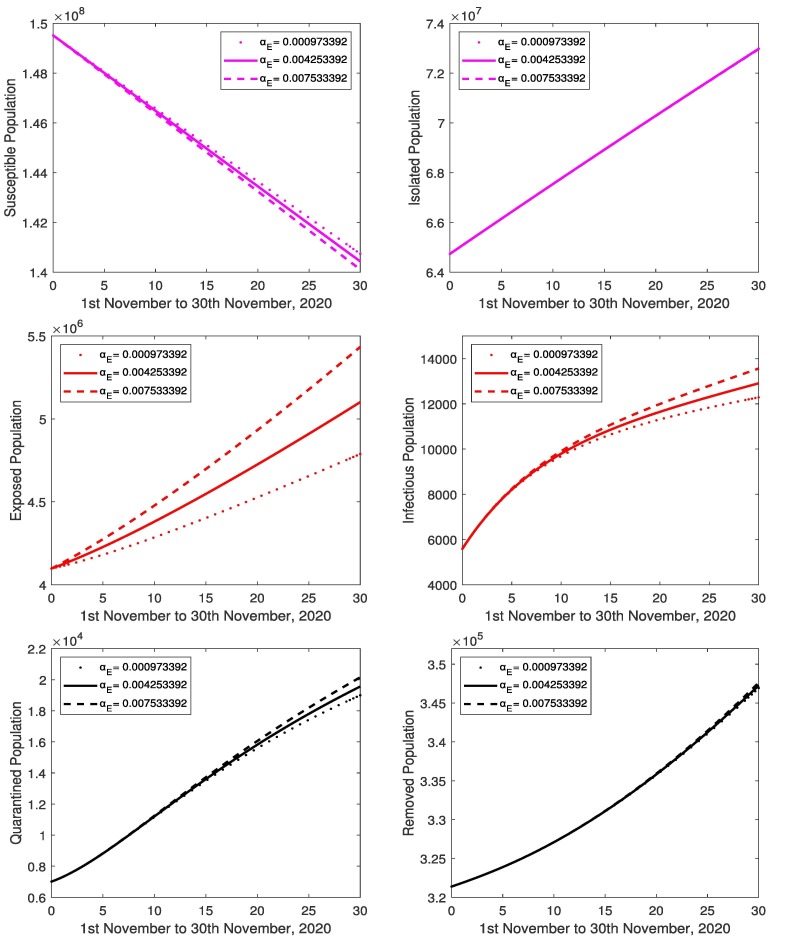
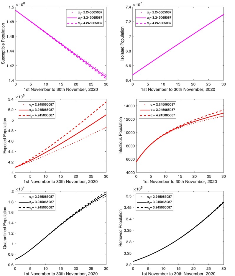
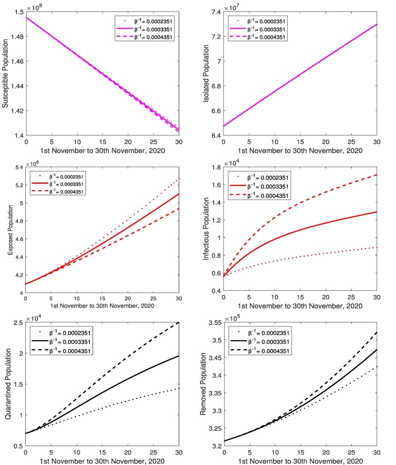
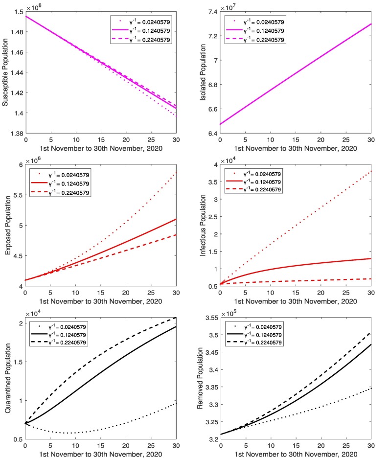
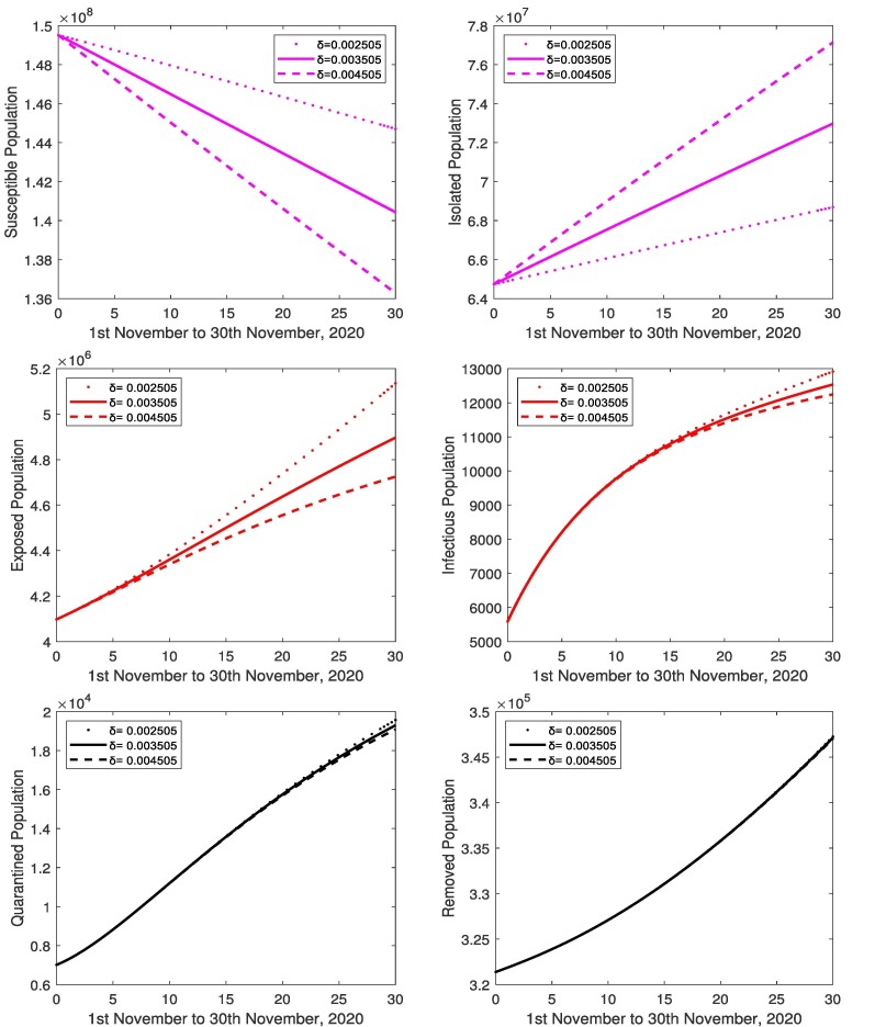
The focus of this section is to study the effects of parameters by changing one parameter while keeping all other parameters fixed. The value of ${\alpha }_E$ transmission rate of the exposed cases to susceptible is varied (0.00163998, 0.00425339, 0.00695208) and all the others parameter values are kept fixed. The variation of susceptible, isolated, exposed, infectious, quarantined and removed population are shown in Fig. 8 . It is found that as the quantitative values of ${\alpha }_E$ increase, the number of infected population also increases along with the increase in number of exposed, quarantined and removed population. The susceptible population decreases more rapidly. The decrease in the value of ${\alpha }_E$ shows a decline in the number of infected, due to less number of infected population. There also occurs a decrease in number of exposed, quarantined and removed population. The susceptible population decline slowly and isolated remain constant. Similarly with the increase and decrease in the value of ${\alpha }_I$ transmission rate of the infectious cases to susceptible (2.245065087, 3.245065087, 4.245065087), presented in Fig. 9 . In Fig. 10 , the value of ${\beta }^{-1}$ (latent period) is considered as (0.0004071, 0.0005071, 0.0006071) and all the other values of parameters are unchanged. The increase in ${\beta }^{-1}$ bring the rise in number of infected population. Than the number of susceptible and exposed cases decreases, and increase in quarantined and removed cases, isolated population remain constant and vice versa. In Fig. 11 , the value of ${\gamma }^{-1}$ (quarantine delay) is considered as (0.00710579, 0.10710579, 0.20710579) and all the other values of parameters are unchanged. The increase in ${\gamma }^{-1}$ bring the fall in number of infected population. Similarly the number of susceptible and exposed cases decreases, and increase in quarantined and removed cases, isolated population remain constant and vice versa. In Fig. 12 , the value of $\delta$ (protection rate) is varied as (0.002505, 0.003505, 0.004505) and all the other values of parameters are unchanged. The increase in $\delta$ bring the fall in number of infected population. Similarly the number of susceptible, exposed, quarantined and removed cases are decreasing and vice versa.

Fig. 8.

Variations of the susceptible, isolated, exposed, infectious, quarantined and removed population for the different values of ${\alpha }_E$. The values of other parameters are ${\alpha }_I=3.245065087,{\beta }^{-1}=0.0003351,{\gamma }^{-1}=0.1240579,\delta =0.003505,r=0.058306850$ and $d=0.00414502$.

Fig. 9.

Variations of the susceptible, isolated, exposed, infectious, quarantined and removed population for the different values of ${\alpha }_I$. The values of other parameters are ${\alpha }_E=0.004253392,{\beta }^{-1}=0.0003351,{\gamma }^{-1}=0.1240579,\delta =0.003505,r=0.058306850$ and $d=0.00414502$.

Fig. 10.

Variations of the susceptible, isolated, exposed, infectious, quarantined and removed population for the different values of ${\beta }^{-1}$. The values of other parameters are ${\alpha }_E=0.004253392,{\alpha }_I=3.245065087,{\gamma }^{-1}=0.1240579,\delta =0.003505,r=0.058306850$ and $d=0.00414502$.

Fig. 11.

Variations of the susceptible, isolated, exposed, infectious, quarantined and removed population for the different values of ${\gamma }^{-1}$. The values of other parameters are ${\alpha }_E=0.004253392,{\alpha }_I=3.245065087,{\beta }^{-1}=0.0003351,\delta =0.003505,r=0.058306850$ and $d=0.00414502$.

Fig. 12.

Variations of the susceptible, isolated, exposed, infectious, quarantined and removed population for the different values of $\delta$. The values of other parameters are ${\alpha }_E=0.004253392,{\alpha }_I=3.245065087,{\beta }^{-1}=0.0003351,{\gamma }^{-1}=0.1240579,r=0.058306850$ and $d=0.00414502$.

In this proposed model, we introduce ${\alpha }_E$ (transmission rate of the exposed to susceptible), ${\alpha }_I$ (transmission rate of the infectious to susceptible), and $\delta$ (protection rate). The value of these parameters in the current situation is 0.004253392, 3.245065087, and 0.003505 respectively. If the values of ${\alpha }_E,{\alpha }_I$, and $\delta$ are less than 0.001, 0.1, and greater than 0.010 respectively then the minimum number of new cases will report (Safe Zone). If the values of ${\alpha }_E,{\alpha }_I$, and $\delta$ are greater than 0.01, 5.0, and less than 0.0001 respectively then the maximum number of new cases will report (Danger Zone).

Test Problem 2: Italy

In the early stages, Italy was the 1st European nation that was affected from COVID-19. The northern Italy was mainly affected. On 30th January, 2020, two Chinese tourists were reported with positive test. After this, on 21st February, 2020 two more cases were reported. The number of deaths in the Lombardy region alone, is greater than the number of deaths in China. Italy became most affected region of the world. We see that one time Italian government controlled the spreading of coronavirus. Now, Italy is facing second wave of coronavirus that is more stronger than the first wave. During first coronavirus wave from 21st February, 2020 to 30th June, 2020, Italy faces 2,40,578 positive cases, 84.5% people recovered and 15.5% people died. Up to 30th November, there were total 16,01,554 positive cases, at the same time 93.2% people recovered from coronavirus and 6.8% people died due to coronavirus.

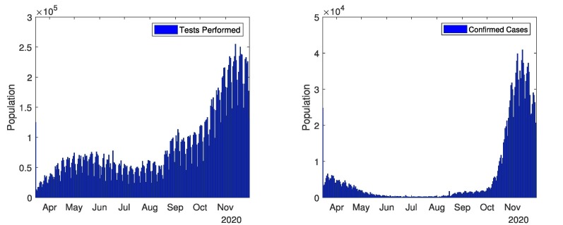
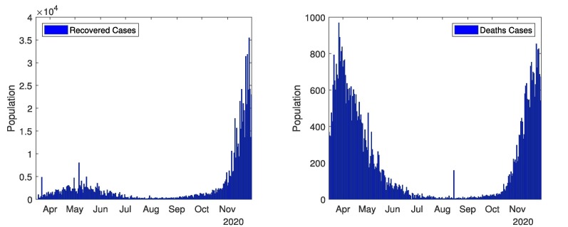
The current complete overview of COVID-19 in Italy shown in Fig. 13 and Fig. 14 . These figures represent the real data of tests performed, confirmed cases, deaths cases and recovered cases. Data related to COVID-19 cases of Italy are taken from different sources [40], [41], [44]. Fig. 13 (first graph) depicts the total number of test performed from 15th March, 2020 to 30th November, 2020.In total 2,19,45,099 tests performed till 30th November, 2020. Fig. 13 (second graph) represents confirmed cases from 15th March, 2020 to 30th November, 2020. Coronavirus start from 21st February in Italy, and continuously increased till April, and then decreased till June. One time coronavirus cases become approximately zero. In September, again coronavirus started to spread in all over Italy, and rapidly increased in confirmed cases from mid of October. The total confirmed cases in Italy are 1,601,554 till 30th November, 2020. The confirmed cases are still increasing. The government closed all the public points, implemented a strict lockdown and aware the masses to follows the SOPs. Due to government polices, the COVID-19 remained in control from end of May to October. In September, the government took off the lockdown and coronavirus spread again from October. Fig. 14 (first graph) represents recovered cases from 15th March, 2020 to 30th November, 2020. There were most recovered cases in April and May during the 1st wave of coronavirus. In total 7,57,507 recovered cases till 30th November, 2020. Fig. 14 (second graph) represents deaths from 15th March, 2020 to 30th November, 2020. As most cases were observed in April, thus most deaths occurred in April (highest 602 in one day and total 15,539 in month). The total deaths till 30th November, 2020 are 55,576.

Fig. 13.

In Italy: Tests performed and confirmed cases.

Fig. 14.

In Italy: Recovered cases and deaths Cases.

The model Eqs. (1), (2), (3), (4), (5), (6) are solved using RK4. The simulated results of model equations (c.f Eqs. (1), (2), (3), (4), (5), (6)) are presented. For the estimation of the values of parameters the statistics terminologies are used.

Problem   1:

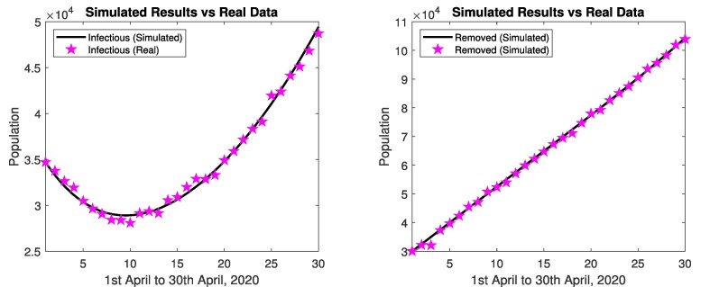
Fig. 15 represents comparison of simulated results and real data of infectious and removed cases from 1st April, 2020 to 30 April, 2020 (during 1st coronavirus wave). The simulated results are close to the real data in infectious and removed cases as depicted in Fig. 15.

Fig. 15.

In Italy: Simulated results and real data of April 2020.

Problem   2:

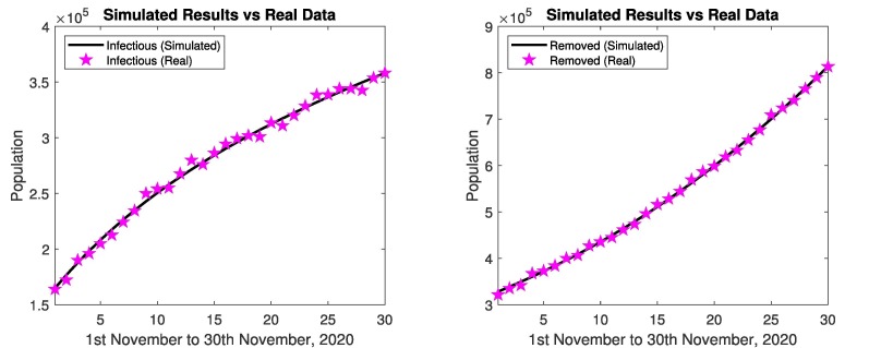
Mostly in Italy maximum coronavirus cases w.r.t all over the World were reported during first wave and than decreasing day by day. Most patients were recovering from disease but second wave of coronavirus started.

Fig. 16 represents the simulated results and real data of infectious and removed cases from 1st November to 30th November, 2020. The simulated results are close to the real data in infectious and removed cases, relative errors are given in Table 4, Table 5 .

Fig. 16.

In Italy: Simulated results and real data of November 2020.

Table 4.

Study of relative errors of infectious cases for Italy.

Date	Relative errors	Date	Relative errors	Date	Relative errors
1st Nov	0.005837104	11th Nov	0.010989666	21st Nov	0.020836
2nd Nov	0.025797482	12th Nov	0.010825995	22nd Nov	0.006932
3rd Nov	0.011612837	13th Nov	0.029570628	23rd Nov	0.004111
4th Nov	0.01128946	14th Nov	0.006934419	24th Nov	0.019193
5th Nov	0.015502215	15th Nov	0.007492452	25th Nov	0.006465
6th Nov	0.022972174	16th Nov	0.01461214	26th Nov	0.008803
7th Nov	0.009043897	17th Nov	0.01080272	27th Nov	0.004014
8th Nov	0.0017352	18th Nov	0.001021074	28th Nov	0.020968
9th Nov	0.028329254	19th Nov	0.020118045	29th Nov	0.000759
10th Nov	0.014030874	20th Nov	0.003738704	30th Nov	0.000106

Table 5.

Study of relative errors of removed cases for Italy.

Date	Relative errors	Date	Relative errors	Date	Relative errors
1st Nov	0.021289	11th Nov	0.009953	21st Nov	0.000747483
2nd Nov	0.010234	12th Nov	0.005955	22nd Nov	0.008041242
3rd Nov	0.022164	13th Nov	0.012284	23rd Nov	0.004971367
4th Nov	0.018508	14th Nov	0.002667	24th Nov	0.003336089
5th Nov	0.001966	15th Nov	0.009950	25th Nov	0.012826909
6th Nov	0.000210	16th Nov	0.001081	26th Nov	0.003136554
7th Nov	0.010121	17th Nov	0.000732	27th Nov	0.004863319
8th Nov	0.005261	18th Nov	0.012080	28th Nov	0.00176126
9th Nov	0.012356	19th Nov	0.010885	29th Nov	0.000366077
10th Nov	0.000081	20th Nov	0.000919	30th Nov	0.000256919

Fig. 17 represents the simulated results of the model (susceptible, isolated, exposed, infectious, quarantined and removed cases) from 1st to 30th November, 2020. The results shows the decrease in susceptible population and increase in infected and removed population. Similarly the exposed cases and isolated cases increases. The affected people are recovering from disease. When the people follow the SOPs, then decrease in infectious and quarantined cases, and increase in isolation. When the government strictly implements the SOPs against the spread of coronavirus then isolated population increases fastly.

Fig. 17.

In Italy: Simulated results of susceptible, isolated, exposed, infectious, quarantined and removed cases from 1st November to 30th November, 2020.

Table 4 represents the relative errors from 1st November to 30th November, 2020 of infectious cases. We see that the relative errors are less than 1 for all days. Table 5 represents relative errors from 1st November to 30th November, 2020 of removed cases. We see that the relative errors are less than 1 for all days, which verify the correctness of model formulation. The developed mathematical model can be helpful to measure the coronavirus situations.

Problem   3: Prediction for Next 6 Months

The prediction of COVID-19 using the mathematical model is presented. Fig. 18 represents the prediction of COVID-19 for 180 days. The simulated results by developed model of COVID-19 (1st December, 2020 to 30th May, 2021) are presented. The results show that the number of infected cases are increasing almost 43%. As the infected increases, the suspected decreases 79%, which is clearly depicted in Fig. 18. Furthermore, Fig. 18 shows that number of removed cases are increasing. According to the results, the infected population due to COVID-19 will increase then decrease from April 2021. The government has to implement strict strategies such as smart lock-down, reduction of timings in shops etc to control the disease. If people follow SOPs than coronavirus will be controlled otherwise its not possible.

Fig. 18.

In Italy: Simulated results of susceptible, isolated, exposed, infectious, quarantined and removed cases from 1st December, 2020 to 30th May, 2021.

In this proposed model, we introduce ${\alpha }_E$ (transmission rate of the exposed to susceptible), ${\alpha }_I$ (transmission rate of the infectious to susceptible), and $\delta$ (protection rate). The value of these parameters in the current situation is 0.0273207, 0.1211833, and 0.0050605 respectively. If the values of ${\alpha }_E,{\alpha }_I$, and $\delta$ are less than 0.0001, 0.010, and greater than 0.020 respectively then the minimum number of new cases will report (Safe Zone). If the values of ${\alpha }_E,{\alpha }_I$, and $\delta$ are greater than 0.100, 1.00, and less than 0.0010 respectively then the maximum number of new cases will report (Danger Zone).

Test Problem 3: Japan

The 1st outbreak of the COVID-19 in the Japan was reported on 16th January, 2020 in a resident of Kanagawa Prefecture. He came back from Wuhan, China. The 2nd outbreak was reported between 11th to 23rd March, 2020 from returners and travelling passengers, who came from the United States and Europe. The major cause of spreading coronavirus in country is due to Europe and China. Japan government took action on early stages, the Prime Minister Shinzo Abe requested to the closure off all the Japanese schools on 27th Feb, 2020. In Japan, the death rate is lowest per capita with respect to the developed world. Now again Japan faces increasing in coronavirus in all over the country. During first coronavirus wave from 23rd March, 2020 to 30th June, 2020, Italy faces 18,612 positive cases, 94.5% people recovered and 5.5% people died. In second coronavirus wave till 30th September, 2020, Italy faces 83,591 positive cases, 97.9% people recovered and 2.1% people died. Up to 30th November, there were total 1,49,962 positive cases, at the same time 98.4% people recovered from coronavirus and 1.6% people died due to COVID-19.

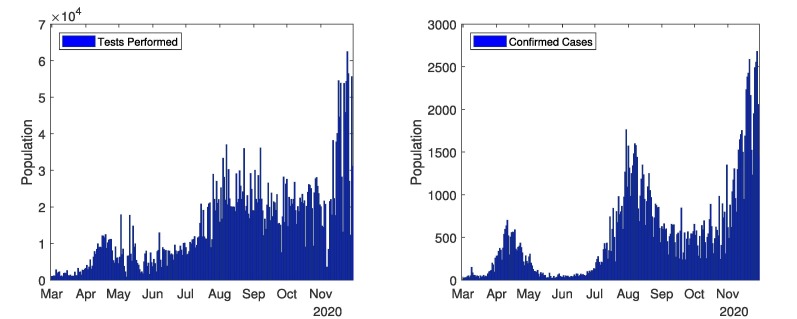
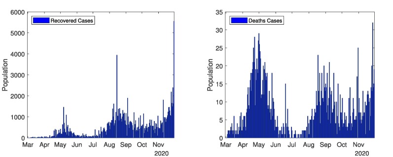
The current and complete overview of COVID-19 in all over Japan shown in Fig. 19, Fig. 20 . These figures represent the real data of tests performed, confirmed cases, deaths cases and recovered cases. Data related to COVID-19 cases of Japan are taken from different sources [40], [41], [45]. Fig. 19 (first graph) represents, the test performed from 1st March, 2020 to 30th November, 2020. Mostly tests are performed in August. The total tests performed till 30th November, 2020 are 41,06,169. Fig. 19 (second graph) represents confirmed cases from 1st March, 2020 to 30th November, 2020. Coronavirus start from 23rd March in Japan, and continuously increased till mid of April, then decreasing till July. In July, again coronavirus started to spread in Japan. There were most confirmed cases in August (highest 1762 in one day and total 32,162 in a month). The total confirmed cases in Pakistan are 1,49,962 till 30th November, 2020. The confirmed cases are still increasing. The government closed all the public points, implemented a strict lockdown and aware the masses to follows the SOPs. Due to government polices, the COVID-19 remained in control from end of May to July and in September and October. Government of Japan took off the lockdown and coronavirus spread again. When government took the lockdown than coronavirus controlled otherwise started to spread. Fig. 20 (first graph) represents recovered cases from 1st March, 2020 to 30th November, 2020. There were most recovered cases in August, during the 2nd wave of coronavirus. In total 1,27,289 recovered people till 30th November, 2020. Fig. 20 (second graph) represents the number of deaths from 1st March, 2020 to 30th November, 2020. There were most deaths in April and May (highest 29 in one day and total 832 in two month). In total 2,076 deaths till 30th November, 2020.

Fig. 19.

In Japan: Tests performed and confirmed cases.

Fig. 20.

In Japan: Recovered cases and deaths Cases.

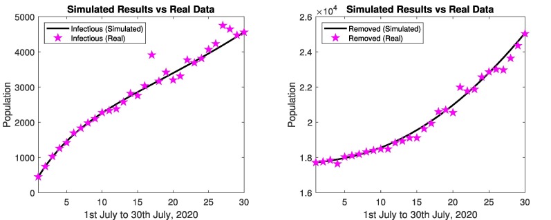
The model given in Eqs. (1), (2), (3), (4), (5), (6) are solved using RK4 for Japan. The simulated results of model equations (c.f Eqs. (1), (2), (3), (4), (5), (6)) are presented. For the estimation of the values of parameters the statistics terminologies are used. The comparison of simulated results and real data of infectious and removed cases are provided in graphs.

Problem   1:

Fig. 21 represents the comparison of simulated results and real data of infectious and removed cases from 1st July, 2020 to 30th July, 2020 of Japan. The simulated results are close to the real data in infectious and removed cases as depicted in Fig. 21. Problem 2:

Fig. 21.

In Japan: Simulated results and real data of July 2020.

Fig. 22 represent the simulated results and real data of infectious and removed cases from 1st November to 30th November, 2020. The simulated results are close to the real data in infectious and removed cases, relative errors are given in Table 6, Table 7 .

Fig. 22.

In Japan: Simulated results and real data of November 2020.

Table 6.

Study of relative errors of infectious cases for Japan.

Date	Relative errors	Date	Relative errors	Date	Relative errors
1st Nov	0.021417	11th Nov	0.013667	21st Nov	0.003152
2nd Nov	0.032025	12th Nov	0.025980	22nd Nov	0.011940
3rd Nov	0.062096	13th Nov	0.114169	23rd Nov	0.015773
4th Nov	0.046100	14th Nov	0.007850	24th Nov	0.011560
5th Nov	0.019282	15th Nov	0.066167	25th Nov	0.015211
6th Nov	0.029177	16th Nov	0.010303	26th Nov	0.049499
7th Nov	0.116308	17th Nov	0.024887	27th Nov	0.049959
8th Nov	0.038660	18th Nov	0.052348	28th Nov	0.081207
9th Nov	0.031839	19th Nov	0.046037	29th Nov	0.043064
10th Nov	0.034344	20th Nov	0.002207	30th Nov	0.006499

Table 7.

Study of relative errors of removed cases for Japan.

Date	Relative errors	Date	Relative errors	Date	Relative errors
1st Nov	0.005460839	11th Nov	0.002168027	21st Nov	0.002209304
2nd Nov	0.004118358	12th Nov	0.003456148	22nd Nov	0.000166255
3rd Nov	0.002964324	13th Nov	0.005825422	23rd Nov	0.004016489
4th Nov	0.000982712	14th Nov	0.008252693	24th Nov	7.25122E-05
5th Nov	0.008073763	15th Nov	0.005905965	25th Nov	0.003515107
6th Nov	0.00130152	16th Nov	0.002007694	26th Nov	0.003280727
7th Nov	0.00016718	17th Nov	0.001519254	27th Nov	0.003623707
8th Nov	0.001257024	18th Nov	0.004564607	28th Nov	0.006613595
9th Nov	0.002073573	19th Nov	0.002818295	29th Nov	0.000869262
10th Nov	0.000156779	20th Nov	0.002632602	30th Nov	0.000338695

Fig. 23 represents the simulated results of the model (susceptible, isolated, exposed, infectious, quarantined and removed cases) from 1st November to 30th November, 2020. The results shows the decrease in susceptible population and increase in infected and removed population. Similarly the exposed cases and isolated cases increases. The affected people are recovering from disease. When the people follow the SOPs, then decrease in infectious and quarantined cases, and increase in isolation. When the government strictly implements the SOPs against the spread of coronavirus then isolated population increases fastly.

Fig. 23.

In Japan: Simulated results of susceptible, isolated, exposed, infectious, quarantined and removed cases from 1st November to 30th November, 2020.

Table 6 represents the relative errors from 1st November to 30th November, 2020 of infectious cases. We see that the relative errors are less than 1 for all days. Table 7 represents relative errors from 1st November to 30th November, 2020 of removed cases. We see that the relative errors are less than 1 for all days, which verify the correctness of model formulation. The developed mathematical model can be helpful to measure the coronavirus situations.

Problem   3: Prediction for Next 6 Months

The prediction of COVID-19 using the mathematical model is presented. Fig. 24 represents the prediction of COVID-19 for 180 days. The simulated results by developed model of COVID-19 (1st December, 2020 to 30th May, 2021) are presented. The results show that the number of infected cases are increasing almost 491%. As the infected increases, the suspected decreases 50%, which is clearly depicted in Fig. 24. Fig. 24 depicts that number of removed cases are increasing. According to the results, the infected population due to COVID-19 will increase. The government has to implement strict strategies such as smart lock-down, reduction of timings in shops etc to control the disease. If people follow SOPs than coronavirus will be controlled otherwise its not possible. In this proposed model, we introduce ${\alpha }_E$ (transmission rate of the exposed to susceptible), ${\alpha }_I$ (transmission rate of the infectious to susceptible), and $\delta$ (protection rate). The value of these parameters in the current situation is 0.2416577, 0.1091595, and 0.0017900 respectively. If the values of ${\alpha }_E,{\alpha }_I$, and $\delta$ are less than 0.1, 0.01, and greater than 0.0030 respectively then the minimum number of new cases will report (Safe Zone). If the values of ${\alpha }_E,{\alpha }_I$, and $\delta$ are greater than 0.5, 1.5, and less than 0.0005 respectively then the maximum number of new cases will report (Danger Zone).

Fig. 24.

In Japan: Simulated results of susceptible, isolated, exposed, infectious, quarantined and removed cases from 1st December, 2020 to 30th May, 2021.

Test Problem 4: Spain

The virus was firstly confirmed in Spain on 31st January, 2020 from a German tourist. On 13th March, 2020 coronavirus spread in all the 50 provinces of the country. The government of Spain imposed lockdown on 14th March, 2020. The Spain also had become world highest reported rate of coronavirus infection for doctors and nurses. Now Spain has lifted strictest lockdowns and has given permission to people for movement in country and has opened the borders to some countries. During first coronavirus wave from 31st January, 2020 to 30th June, 2020, Italy faces 2,54,117 positive cases, 85.2% people recovered and 14.8% people died. Up to 30th November, there were total 17,02,328 positive cases, at the same time 96.9% people recovered from coronavirus and 3.1% people died due to coronavirus.

The current complete overview of COVID-19 in all over the Spain shown in Figs. 25 and 26 . These Figures represents the real data of tests performed, confirmed cases, deaths cases and recovered cases. Data related to COVID-19 cases of Pakistan are taken from different sources [40], [41], [46]. Fig. 25 (first graph) depicts the number of test performed from 16th March, 2020 to 30th November, 2020. Mostly tests are performed from September. The total test performed till 30th November, 2020 are 1,87,72,604. Fig. 25 (second graph) represents the confirmed cases from 16th March, 2020 to 30th November, 2020. Coronavirus start from 31st January in Spain, and continuously increasing till April, and decreasing till mid of May. There were most confirmed cases in Spain during first coronavirus wave from 20th March to 20th April (highest 9,222 in one day and total 1,79,660 in 30 days). There were normal coronavirus cases in May and June. In Spain second coronavirus wave started from August and rapidly increases in confirmed cases from mid of October. The total confirmed cases in Spain are 17,02,328 till 30th November, 2020. The confirmed cases are still increasing. This figure also depicts the effects of governmental actions, when Spain faces 1st wave of COVID-19 then government close all the public points, implements a strict lockdown and aware the masses to follows the SOPs. Due to government polices, the COVID-19 remained in control from end of May to August. In August, the government took off the lockdown and coronavirus spread again. Fig. 26 (first graph) represents recovered cases from 16th March, 2020 to 30th November, 2020. There were most recovered cases in September and October. In total 14,16,001 recovered cases till 30th November, 2020. Fig. 26 (second graph) represents increasing the number of deaths from 16th March to 30th November, 2020. As most cases were observed in April and November thus most deaths occurred in April and November. In total 46,038 deaths till 30th November, 2020.

Fig. 25.

In Spain: Tests performed and confirmed cases.

Fig. 26.

In Spain: Recovered cases and deaths Cases.

The model given in Eqs. (1), (2), (3), (4), (5), (6) are solved using RK4 for Spain. The simulated results of model equations (c.f. Eqs. (1), (2), (3), (4), (5), (6)) are presented. For the estimation of the values of parameters the statistics terminologies are used. The parameters values are given in Table 1. The comparison of simulated results and real data of infectious and removed cases are provided in graphs.

Problem   1:

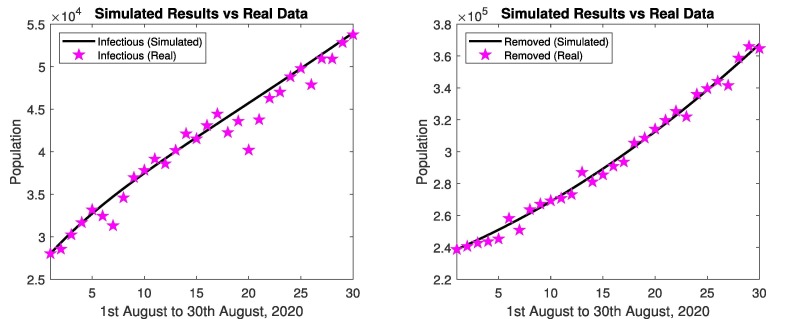
Fig. 27 represents the comparison of simulated results and real data of infectious and removed cases from 1st August, 2020 to 30th August, 2020 of Spain. The simulated results are close to the real data in infectious and removed cases as depicted in Fig. 27.

Fig. 27.

In Spain: Simulated results and real data of August 2020.

Problem   2:

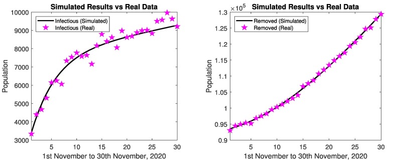
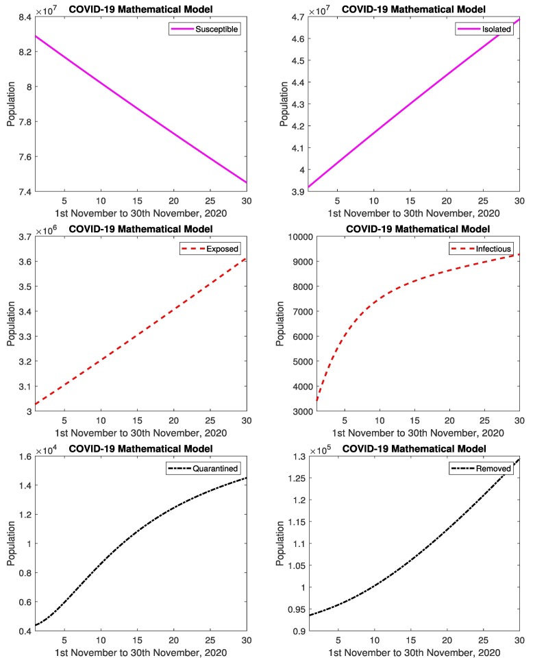
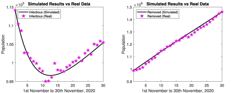
Fig. 28 represents the simulated results and real data of infectious and removed cases from 1st November to 30th November, 2020. The simulated results are close to the real data in infectious and removed cases, relative errors are given in Table 8, Table 9 . Figs. 29 represents the simulated results of the model (susceptible, isolated, exposed, infectious, quarantined and removed cases) from 1st November to 30th November, 2020. The results shows the decrease in susceptible population and increase in infected population, after decrease. The exposed cases, removed cases and isolated cases increases. The affected people are recovering from disease. The quarantined population decreases. When the people follow the SOPs, then decrease in infectious and quarantined cases, and increase in isolation. When the government strictly implements the SOPs against the spread of coronavirus then isolated population increases fastly.

Fig. 28.

In Spain: Simulated results and real data of November 2020.

Table 8.

Study of relative errors of infectious cases for Spain.

Date	Relative errors	Date	Relative errors	Date	Relative errors
1st Nov	0.000014	11th Nov	0.018504	21st Nov	0.009561
2nd Nov	0.001751	12th Nov	0.015874	22nd Nov	0.012454
3rd Nov	0.014795	13th Nov	0.005287	23rd Nov	0.002167
4th Nov	0.017023	14th Nov	0.031464	24th Nov	0.011541
5th Nov	0.003007	15th Nov	0.011762	25th Nov	0.012931
6th Nov	0.006194	16th Nov	0.007177	26th Nov	0.004235
7th Nov	0.010685	17th Nov	0.000956	27th Nov	0.015973
8th Nov	0.015374	18th Nov	0.008230	28th Nov	0.006864
9th Nov	0.008847	19th Nov	0.008324	29th Nov	0.010380
10th Nov	0.006876	20th Nov	0.011750	30th Nov	0.000408

Table 9.

Study of relative errors of removed cases for Spain.

Date	Relative errors	Date	Relative errors	Date	Relative errors
1st Nov	0.00000213	11th Nov	0.000217077	21st Nov	0.016671331
2nd Nov	0.012492074	12th Nov	0.004615424	22nd Nov	0.012332486
3rd Nov	0.02101917	13th Nov	0.002098478	23rd Nov	0.011836044
4th Nov	0.026333605	14th Nov	5.86819E-06	24th Nov	0.015308041
5th Nov	0.015092313	15th Nov	0.002903759	25th Nov	0.015711163
6th Nov	0.016036556	16th Nov	0.005694897	26th Nov	0.012592594
7th Nov	0.010022301	17th Nov	0.002278282	27th Nov	0.008109654
8th Nov	0.013570866	18th Nov	0.001777407	28th Nov	0.003540895
9th Nov	0.001216548	19th Nov	0.022646527	29th Nov	0.001132337
10th Nov	0.004912528	20th Nov	0.019578519	30th Nov	0.000021565

Fig. 29.

In Spain: Simulated results of susceptible, isolated, exposed, infectious, quarantined and removed cases from 1st November to 30th November, 2020.

Table 8 represents the relative errors from 1st November to 30th November, 2020 of infectious cases. We see that the relative errors are less than 1 for all days. Table 9 represents relative errors from 1st November to 30th November, 2020 of removed cases. We see that the relative errors are less than 1 for all days, which verify the correctness of model formulation. The developed mathematical model can be helpful to measure the coronavirus situations.

Problem   3: Prediction for Next 6 Months

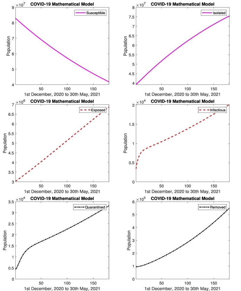
The prediction of COVID-19 using the mathematical model is presented. Fig. 30 represents the prediction of COVID-19 for 180 days. The simulated results by developed model of COVID-19 (1st December, 2020 to 30th May, 2021) are presented. The results show that the number of infected cases are increasing almost 34%, after a small decrease. As the infected increases, the suspected decreases 58%, which is clearly depicted in Fig. 30. Furthermore, Fig. 30 shows that the number of removed cases are increasing. According to the results, the infected population due to COVID-19 will increase. The government has to implement strict strategies such as smart lock-down, reduction of timings in shops etc to control the disease. If people follow SOPs than coronavirus will be controlled otherwise its not possible.

Fig. 30.

In Spain: Simulated results of susceptible, isolated, exposed, infectious, quarantined and removed cases from 1st December, 2020 to 30th May, 2021.

In this proposed model, we introduce ${\alpha }_E$ (transmission rate of the exposed to susceptible), ${\alpha }_I$ (transmission rate of the infectious to susceptible), and $\delta$ (protection rate). The value of these parameters in the current situation is 0.0261309, 0.2619047, and 0.0018373 respectively. If the values of ${\alpha }_E,{\alpha }_I$, and $\delta$ are less than 0.007, 0.150, and greater than 0.009 respectively then the minimum number of new cases will report (Safe Zone). If the values of ${\alpha }_E,{\alpha }_I$, and $\delta$ are greater than 0.15, 0.90, and less than 0.0005 respectively then the maximum number of new cases will report (Danger Zone).

Conclusion

In this study, developed model was solved using numerical methods. The model contains system of ODEs which incorporate the human population (susceptible, exposed, infectious, quarantined, removed (recover and death) and also, we include isolated cases (due to govt action)). Runge Kutta of order four (RK4) was applied to acquire the numerical solution. Four test problems were considered with publicly available data, simulated data is then compared with the real data in order to validate proposed model. It is found that numerically obtained results using proposed model are very close to the real data. It is also observed that for some conditions, irregularities in the real data was observed which was hard to cover by numerical methods. However, these variations are accommodated in the proposed model with the help of parametric values. Proposed model is validated on the basis of test problems and predict the future condition of Pakistan, Italy, Japan and Spain. simulation results proposed that, for Pakistan, if the values of ${\alpha }_E,{\alpha }_I$, and $\delta$ are less than 0.001, 0.1, and greater than 0.010 respectively then the minimum number of new cases will report (Safe Zone). If the values of ${\alpha }_E,{\alpha }_I$, and $\delta$ are greater than 0.01, 5.0, and less than 0.0001 respectively then the maximum number of new cases will report (Danger Zone). The studies also proposes statistics for Italy that, if the values of ${\alpha }_E,{\alpha }_I$, and $\delta$ are less than 0.0001, 0.010, and greater than 0.020 respectively then the minimum number of new cases will report (Safe Zone). If the values of ${\alpha }_E,{\alpha }_I$, and $\delta$ are greater than 0.100, 1.00, and less than 0.0010 respectively then the maximum number of new cases will report (Danger Zone). The studies also presents statistics for Japan that, if the values of ${\alpha }_E,{\alpha }_I$, and $\delta$ are less than 0.1, 0.01, and greater than 0.0030 respectively then the minimum number of new cases will report (Safe Zone). If the values of ${\alpha }_E,{\alpha }_I$, and $\delta$ are greater than 0.5, 1.5, and less than 0.0005 respectively then the maximum number of new cases will report (Danger Zone). Finally for Spain it is proposed that, if the values of ${\alpha }_E,{\alpha }_I$, and $\delta$ are less than 0.007, 0.150, and greater than 0.009 respectively then the minimum number of new cases will report (Safe Zone). If the values of ${\alpha }_E,{\alpha }_I$, and $\delta$ are greater than 0.15, 0.90, and less than 0.0005 respectively then the maximum number of new cases will report (Danger Zone). Furthermore, parametric study was performed. The study recommends to take this epidemic decease as a serious decease. Effects of this decease can be minimized by following all the SOP’s governed by WHO and local governments of the region. Also to minimize all the unnecessary activities along with proper hygiene. It is also concluded that the developed model can be used to analyze the transmission of COVID-19 in other regions.

Future recommendations

This comprehensive study for four different countries is analysed for key parameters such as transmission coefficient of exposed cases to susceptible cases, transmission coefficient of infectious cases to susceptible, and govt actions to restrict the spread of pandemic. It is obvious that the transmission coefficients should have as less values as possible and govt actions should have large values to control the disease. The range of safe and danger zones are also highlighted in this paper.

Funding

This work was supported by National Natural Science Foundation of China (No. 71601072) and Key Scientific Research Project of Higher Education Institutions in Henan Province of China (No. 20B110006).

CRediT authorship contribution statement

Shumaila Javeed: Conceptualization, Formal analysis, Methodology, Investigation, Supervision, Project administration, Writing - original draft. Subtain Anjum: Visualization, Data curation, Formal analysis, Investigation, Writing - original draft. Khurram Saleem Alimgeer: Writing - original draft, Writing - review & editing, Validation, Software, Investigation, Writing - review & editing. M. Atif: Supervision, Project administration, Resources, Funding acquisition. Mansoor Shaukat Khan: Visualization, Data curation, Writing - original draft. W. Aslam Farooq: Visualization, Data curation, Software. Atif Hanif: Visualization, Data curation, Software, Investigation. Hijaz Ahmad: Validation, Supervision, Project administration, Funding acquisition. Shao-Wen Yao: Supervision, Project administration, Funding acquisition.

Declaration of Competing Interest

The authors declare that they have no known competing financial interests or personal relationships that could have appeared to influence the work reported in this paper.

References

- 1.Li Q., Guan X., Wu P., Wang X., Zhou L., Tong Y. Early transmission dynamics in Wuhan, China, of novel coronavirus-infected pneumonia. N Engl J Med. 2020 doi: 10.1056/NEJMoa2001316. [DOI] [PMC free article] [PubMed] [Google Scholar]
- 2.WHO statement regarding the outbreak of novel coronavirus (2019-nCoV); 2020. Available from:https://www.who.int/news-room/detail/30-01-2020-statement-on-the-second-meeting-of-the-international-health-regulations-(2005)-emergency-committee-regarding-the-outbreak-of-novel-coronavirus-/ (2019-ncov).
- 3.National Health Commission of the People’s Republic of China, Update on the novel coronavirus pneumonia outbreak. http://www.nhc.gov.cn/xcs/yqtb/list_ gzbd.shtml.
- 4.World Health Organization, Coronavirus disease (COVID-2019) situation reports;www.who.int/emergencies/diseases/novelcoronavirus-2019/situation-reports/.
- 5.WHO Coronavirus Disease (COVID-19) Dashboard, Globally there have been confirmed cases of COVID-19, including deaths. Available from:https://covid19.who.int/.
- 6.Javeed S., Ahmed A., Ali M.S., Javed M.A. Stability analysis and solutions of dynamical models for dengue. Punjab Univ J Math. 2018;50(2):45–67. [Google Scholar]
- 7.Anderson M. Population biology of infectious diseases: Part 1. Nature. 1979;280:361–367. doi: 10.1038/280361a0. [DOI] [PubMed] [Google Scholar]
- 8.Thieme H.R. Princeton University Press; 2003. Mathematics in population biology. Mathematical biology series. [Google Scholar]
- 9.Luo X, Sh. Feng, Yang J, et al. Analysis of potential risk of COVID-19 infections in China based on a pairwise epidemic model; 2020. doi:10.20944/preprints202002.0398.v1.
- 10.Peng L, Yang W, Zhang D, et al. Epidemic analysis of COVID-19 in China by dynamical modeling. arXiv:2002.06563 2020; 8.
- 11.Shao N., Zhong M., Yan Y. Dynamic models for coronavirus disease 2019 and data analysis. Math Meth Appl Sci. 2020:1–7. doi: 10.1002/mma.6345. [DOI] [PMC free article] [PubMed] [Google Scholar]
- 12.Chan J.F.-W., Yuan S., Kok K.-H., To K.K.W., Chu H., Yang J. A familial cluster of pneumonia associated with the 2019 novel coronavirus indicating person-to-person transmission: a study of a family cluster. Lancet. 2020;395:514–523. doi: 10.1016/S0140-6736(20)30154-9. [DOI] [PMC free article] [PubMed] [Google Scholar]
- 13.Weston C., Roda W., Varugheseb M. Why is it difficult to accurately predict the COVID-19 epidemic? Infect Dis Model. 2020;5:271–281. doi: 10.1016/j.idm.2020.03.001. [DOI] [PMC free article] [PubMed] [Google Scholar]
- 14.Li Q., Guan X., Wu P. Early transmission dynamics in Wuhan, China, of novel coronavirus–infected pneumonia. New Engl J Med. 2020 29 doi: 10.1056/NEJMoa2001316. [DOI] [PMC free article] [PubMed] [Google Scholar]
- 15.Leung WJT, Leung K. Nowcasting and forecasting the potential domestic and international spread of the 2019-nCoV outbreak originating in Wuhan, China: a modelling study. Lancet 2020;395(10225):689–697. doi:10.1016/S0140-6736(20)30260-9. [DOI] [PMC free article] [PubMed]
- 16.Lin ZS, Ran Q, et al. Preliminary estimation of the basic reproduction number of novel coronavirus (2019-nCoV) in China, from 2019 to 2020: a data-driven analysis in the early phase of the outbreak. Int J Infect Dis 2020;92:214–217. doi:10.1016/j.ijid.2020.01.050. [DOI] [PMC free article] [PubMed]
- 17.Bragazzi T.B., Li N.L. An updated estimation of the risk of transmission of the novel coronavirus (2019-nCov) Infect Dis Model. 2020;5:248–255. doi: 10.1016/j.idm.2020.02.001. [DOI] [PMC free article] [PubMed] [Google Scholar]
- 18.BM. Estimation of the final size of the COVID-19 epidemic. [Preprint.] medRxiv. 2020 Feb. 28. doi:10.1101/2020.02.16.20023606.
- 19.Kermack W.O., McKendrick A.G. A contribution to the mathematical theory of epidemics. Proc R Soc A. 1927;115:700–721. [Google Scholar]
- 20.Anderson R.M., May R.M. Directly transmitted infectious diseases: control by vaccination. Science. 1982;215:1053–1060. doi: 10.1126/science.7063839. [DOI] [PubMed] [Google Scholar]
- 21.Dietz K. Vol. 11. Springer; Berlin: 1976. The incidence of infectious diseases under the influence of seasonal fluctuations. (Lecture Notes in Biomathematics). [Google Scholar]
- 22.Tang B., Wang Xia, Li Qian, Bragazzi Nicola Luigi, Tang Sanyi, Xiao Yanni, Wu Jianhong. Estimation of the transmission risk of the 2019-ncov and its implication for public health interventions. J Clin Med. 2020;9(2) doi: 10.3390/jcm9020462. [DOI] [PMC free article] [PubMed] [Google Scholar]
- 23.Tang B., Bragazzi Nicola Luigi, Li Qian, Tang Sanyi, Xiao Yanni, Wu Jianhong. An updated estimation of the risk of transmission of the novel coronavirus (2019-ncov) Infect Dis Model. 2020 doi: 10.1016/j.idm.2020.02.001. [DOI] [PMC free article] [PubMed] [Google Scholar]
- 24.Clifford S.J., Klepac Petra, Zandvoort Kevin Van, Quilty Billy J., Eggo Rosalind M., Flasche Stefan. Interventions targeting air travellers early in the pandemic may delay local outbreaks of sars-cov-2. medRxiv. 2020 doi: 10.1093/jtm/taaa068. [DOI] [PMC free article] [PubMed] [Google Scholar]
- 25.Parvaiz Ahmad N., Yavuz Mehmet, Qureshi Sania, Zu Jian, Townley Stuart. Modeling and analysis of COVID-19 epidemics with treatment in fractional derivatives using real data from Pakistan. Eur Phys J Plus. 2020;135(10):1–42. doi: 10.1140/epjp/s13360-020-00819-5. [DOI] [PMC free article] [PubMed] [Google Scholar]
- 26.Parvaiz Ahmad N., Owolabi Kolade M., Yavuz Mehmet, Zu Jian. Chaotic dynamics of a fractional order HIV-1 model involving AIDS-related cancer cells. Chaos Solitons Fractals. 2020;140 [Google Scholar]
- 27.Mehmet Y., Sene Ndolane. Stability analysis and numerical computation of the fractional predator–prey model with the harvesting rate. Fractal Fractional. 2020;4(3):35. [Google Scholar]
- 28.Pervaiz Ahmad N., Yavuz M., Zu J. The role of prostitution on HIV transmission with memory: a modeling approach. Alexandria Eng J. 2020;59(4):2513–2531. [Google Scholar]
- 29.YM, Yokus A. Analytical and numerical approaches to nerve impulse model of fractional-order. Numer Methods Partial Differ Equ 2020;36(6):1348–1368.
- 30.YM, Zdemir N. Analysis of an epidemic spreading model with exponential decay law. Math Sci Appl E-Notes 2020;8(1):142–154.
- 31.Khan M.A., Atangana A., Alzahrani E. The dynamics of COVID-19 with quarantined and isolation. Adv Differ Equ. 2020;2020(1):1–22. doi: 10.1186/s13662-020-02882-9. [DOI] [PMC free article] [PubMed] [Google Scholar]
- 32.Qureshi MZ, Memon BR. Assessing the role of quarantine and isolation as control strategies for COVID-19 outbreak: a case study. Chaos Solitons Fractals 2021;144:110655. [DOI] [PMC free article] [PubMed]
- 33.MSS, Qureshi S, Zhao S, Yusuf A, Mustapha UT, He D. Mathematical modeling of COVID-19 epidemic with effect of awareness programs. Infect Dis Model 2021;6:448–460. [DOI] [PMC free article] [PubMed]
- 34.Atangana A., Araz S.İ. Mathematical model of COVID-19 spread in Turkey and South Africa: theory, methods, and applications. Adv Differ Equ. 2020;2020(1):1–89. doi: 10.1186/s13662-020-03095-w. [DOI] [PMC free article] [PubMed] [Google Scholar]
- 35.POJ, Qureshi S, Yusuf A, Al-Shomrani M, Idowu AA. A new mathematical model of COVID-19 using real data from Pakistan. Results Phys 2021;104098. [DOI] [PMC free article] [PubMed]
- 36.Atangana A., Araz S.İ. Modeling and forecasting the spread of COVID-19 with stochastic and deterministic approaches: Africa and Europe. Adv Differ Equ. 2021;2021(1):1–107. doi: 10.1186/s13662-021-03213-2. [DOI] [PMC free article] [PubMed] [Google Scholar]
- 37.Atangana E., Atangana A. Facemasks simple but powerful weapons to protect against COVID-19 spread: can they have sides effects? Results Phys. 2020;103425 doi: 10.1016/j.rinp.2020.103425. [DOI] [PMC free article] [PubMed] [Google Scholar]
- 38.Pervaiz Ahmad N, Yavuz M, Qureshi S, Zu J, Townley S. Modeling and analysis of COVID-19 epidemics with treatment in fractional derivatives using real data from Pakistan. Eur Phys J Plus 2020;135(10):1–42. [DOI] [PMC free article] [PubMed]
- 39.Atangana A. Modelling the spread of COVID-19 with new fractal-fractional operators: Can the lockdown save mankind before vaccination? Chaos Solitons Fractals. 2020;136 doi: 10.1016/j.chaos.2020.109860. [DOI] [PMC free article] [PubMed] [Google Scholar]
- 40.WHO Coronavirus Disease (COVID-19) Dashboard.https://covid19.who.int/.
- 41.Coronavirus Statistiques.https://www.coronavirus-statistiques.com/.
- 42.Coronavirus Update (Live). COVID-19 CORONAVIRUS PANDEMIC.https://www.worldometers.info/coronavirus/.
- 43.COVID-19 Health Advisory Platform by Ministry of National Health, Pakistan.http://covid.gov.pk/.
- 44.Covid-19, situation in Italy – Ministero della Salute.http://www.salute.gov.it/portale/nuovocoronavirus/homeNuovoCoronavirus.jsp?lingua=english.
- 45.Japan’s Response to the Novel Coronavirus Disease: Declaration of a State of Emergency. COVID-19 Information and Resouces.https://corona.go.jp/en/.
- 46.Spain Coronavirus Map and Case Count.https://www.nytimes.com/interactive/2020/world/europe/spain-coronavirus-cases.html.
- 47.Hethcote H. The mathematics of infectious diseases. SIAM Rev. 2000;42:599–653. [Google Scholar]