Cega: a single particle segmentation algorithm to identify moving particles in a noisy system

Abstract

Improvements to particle tracking algorithms are required to effectively analyze the motility of biological molecules in complex or noisy systems. A typical single particle tracking (SPT) algorithm detects particle coordinates for trajectory assembly. However, particle detection filters fail for data sets with low signal-to-noise levels. When tracking molecular motors in complex systems, standard techniques often fail to separate the fluorescent signatures of moving particles from background signal. We developed an approach to analyze the motility of kinesin motor proteins moving along the microtubule cytoskeleton of extracted neurons using the Kullback-Leibler divergence to identify regions where there are significant differences between models of moving particles and background signal. We tested our software on both simulated and experimental data and found a noticeable improvement in SPT capability and a higher identification rate of motors as compared with current methods. This algorithm, called Cega, for “find the object,” produces data amenable to conventional blob detection techniques that can then be used to obtain coordinates for downstream SPT processing. We anticipate that this algorithm will be useful for those interested in tracking moving particles in complex in vitro or in vivo environments.

INTRODUCTION

Developments in fluorescence imaging methods, such as total internal reflection fluorescence (TIRF) microscopy, have revolutionized live cell microscopy, allowing for monitoring of dynamic events in a variety of biological systems. TIRF uses an evanescent wave generated by reflecting a laser beam at a critical angle to illuminate fluorophores within a very small distance (∼100 nm) from the surface of a glass coverslip. The high signal-to-noise achieved by this method improves spatiotemporal resolution over conventional imaging techniques, allowing the monitoring of fluorescent single molecules, molecular complexes, and organelles with nanometer precision on subsecond time scales. TIRF microscopy has been widely used to investigate the movement of molecular motors such as kinesin, dynein, and myosin on their corresponding cytoskeletal tracks in purified systems and cells (Vale et al., 1996; Pierce et al., 1997; Belyy and Yildiz, 2014).

There have been substantial efforts to automate the tracking and analysis of the movement of motors and cargos from movies acquired with TIRF microscopy using single particle tracking (SPT) (Meijering et al., 2006; Kalaidzidis, 2007; Jaqaman et al., 2008; Chenouard et al., 2009; Tinevez et al., 2017). SPT describes the set of techniques that select particles of interest and aggregate temporally separated particle coordinates into trajectories. The resulting trajectories are used to study the dynamics of target particles, including processive movements, diffusion, and pausing. Thus, SPT algorithms must be able to select and follow a target with high spatial and temporal fidelity.

The performance of many SPT algorithms are limited by preprocessing steps that remove background signals and noise that can complicate the generation of particle coordinates that are linked into trajectories (Smal and Meijering, 2015). Current tracking software, such as u-track (Jaqaman et al., 2008) and TrackMate (Tinevez et al., 2017), have made great strides to assist in the analysis of typical in vitro systems that use TIRF microscopy to image movement of purified single motors along separated and immobilized tracks in assays where the signal density can be controlled. However, analysis of low signal-to-noise data is difficult if not impossible when using more complex in vitro systems, including engineered cytoskeletal bundles and extracted cytoskeletal systems where bidirectional transport occurs. Images and times series acquired from these more complex in vitro systems include substantial background fluorescence and nuisance particles that complicate application of SPT. The available software implementations of SPT include limited solutions for particle segmentation (Jaqaman et al., 2008; Tinevez et al., 2017) that fail when challenged with data sets that include high levels of background fluorescence, and these algorithms do not consider removal of nuisance particles. In addition, these algorithms fail to accurately track particles that change direction over time and cannot be used in systems that display bidirectional movement.

Here we present a filtering method, Cega, or more appropriately ce:ga (Tohono O’odham for find the object; Mathiot, 1973), for finding and tracking moving fluorescent objects acquired from experiments performed under conditions that include high noise (Figure 1). This method can be substituted into the initial candidate-finding phase of current SPT software and modified for specific data set needs for more accurate particle detection. Our method was developed to analyze data acquired from an EMCCD camera with a back projected pixel size that slightly undersamples the Nyquist rate for the point spread function of a diffraction limited single molecule. First, we calibrated the camera to properly parameterize the noise statistics. Then, we focused on removing nuisance background signal using Cega. We used multiplicative noise statistics to generate two contrasting models that can then be used to augment the signal of moving motors while suppressing the signal from background and nuisance particles. We tested this model with both simulated and experimental data and found that it performed better than current algorithms in tracking molecular motors moving through complex cytoskeletal arrays that contribute high noise levels. The results suggest that this method provides a substantial improvement for low signal-to-noise tracking applications.

FIGURE 1:

Cega workflow. (A) Example time sequence taken from image sequence of kinesin motors moving within an axonal compartment, as well as corresponding tracks calculated after Cega detection. (B) Diagram of Cega steps leading to spot detection. Font between each step indicates values used to process axonal and dendritic data. (C) Image sequence of time points in A after processing with each of Cega’s steps. Image stills represent how data are manipulated at each step. Green arrows indicate moving spots, while red arrows indicate positions of stationary spots. Dim-colored spots in the KL divergence images represent locations of spot detection. Spots in the LoG images represent detected spots, colored by appearance over time. Spots corresponding to the same track are connected with the same colored lines.

RESULTS

Computational strategy and optimization

We developed and used Cega to analyze fluorescently labeled kinesin motors moving along native cellular microtubule networks preserved after extracting membranes and soluble cytosolic components (Figure 1A; see Materials and Methods). These data have substantial background fluorescence along with a high proportion of stationary fluorescent particles due to nonspecific binding that together represent experimentally structured noise. Movies of a truncated GFP-kinesin-1 construct (GFP-K560) moving along microtubule arrays in axonal and dendritic compartments of extracted rat hippocampal neurons were acquired with an EMCCD camera. In axons, kinesin-1 motors move unidirectionally outward from the cell body due to the unipolar arrangement of the microtubule cytoskeletal tracks. However, in dendrites, kinesin-1 motors move in both outward (anterograde) and inward (retrograde) directions due to the mixed polarity of the microtubule cytoskeleton in this part of the neuron. Our goal was to better understand the characteristics of the motile behaviors of kinesin in these environments. However, manual analysis and current SPT software could not reliably distinguish moving motors from nuisance particles in the foreground. Thus, we developed and optimized Cega to analyze these types of data sets.

Here we outline our computational approach to detect and track single fluorescent particles that move bidirectionally from data sets with low signal-to-noise. We first provide an overview, then discuss implementation and optimization of this strategy to analyze single molecule data sets of kinesin motors moving within complex arrays, and conclude with a comparison of Cega to other computational approaches currently available. The normalization procedures and algorithms we developed are described in more detail in Materials and Methods, and the corresponding computer code is available online at https://github.com/prelich/Cega.

Camera calibration

Before application of any algorithm, such as Cega, to detect and identify particles of interest in a time sequence, the detector being used to collect the primary data must be calibrated to ensure pixel intensities are appropriately accounted for when analyzed (Figure 1B). Individual frames of time sequences obtained from cameras and optical sensors typically have noise statistics that are poorly described by a Poisson distribution, as a result of damaged detectors as well as additive and multiplicative noise that accompanies the conversions of photons to digital signals. These factors complicate the use of algorithms to eliminate noise since the data cannot be assumed to have Poisson statistics, and postprocessing data cannot be thresholded reliably (Mortensen and Flyvbjerg, 2016; Mortensen et al., 2010). Thus, camera calibration is required before using Cega to linearly transform the measured pixel intensities of a series of time frames to generate Poisson-like statistics.

Specifically, a stationary object with a constant rate of photon emissions acquired over several frames will register pixel intensities that satisfy the following relation:

1

where, given a constant emission of photons at a pixel i, the time-averaged intensity of the calibrated pixel, <K_i>, is equal to the temporal variance of that calibrated pixel, var(K_i). A Poisson-like distribution is a noninteger analog of the Poisson distribution with units of ‘effective photons’. For our Poisson-like model, the probability of observing some positive real number K given an expected value μ is defined as:

2

The digital signal recovered from a scientific camera will be reported in arbitrary digital units (ADUs) because pixel statistics are dependent on the camera’s configuration. ADUs are sufficient quantities for relative comparisons or when the follow up analysis treats signal noise as irrelevant or predominantly additive. For algorithms that factor in multiplicative noise, the conversion factors that relate a set of ADUs to effective photons are required quantities. Extensive work on CCD (Young et al., 1998) and sCMOS (Huang et al., 2013; Babcock et al., 2019) sensors has demonstrated that statistical regression with a simplified model can effectively recover Poisson-like statistics for estimators that use multiplicative noise models. Given that a scientific camera produces an output signal S_i at pixel i the signal components are defined as:

3

where K_i is the effective photon count, G_i is the multiplicative gain factor on the Poisson-like signal, O_i is the constant mean offset, and R_i is an unbiased random electronic signal generated from the camera read noise. The purpose of camera calibration is to recover G_i, O_i, and var(R_i) and to use these quantities to estimate the effective photons in movies acquired from the calibrated camera. Although the model used to recover K_i is independent of sensor type, calibration techniques will vary among cameras. For EMCCD cameras, pixels are read out in serial so it’s typically assumed that R_i = R, O_i = O, and G_i = G (see Materials and Methods for estimation). The estimated values for the EMCCD camera used to acquire movies of moving kinesin motors were R < 1 effective photon, G = 70 ADU/effective photon, and O = 2293 ADU. The calibrated model we calculated was similar to the initial uncalibrated data after brightness and contrast enhancement and maintained the signal from both moving and stationary particles as well as the background (Table 1; Figure 1C, Calibrated; and Supplemental Videos S1–S4). While we focus here on data obtained from EMCCD cameras, it is possible to adapt this algorithm for data acquired by other camera types including sCMOS cameras. For example, Huang et al. (2013) describe how to adapt filtering algorithms for sCMOS cameras through the use of a Poisson approximation for convolving a Poisson and Gaussian distribution.

TABLE 1:

Cega thresholding values used for experimental data.

Step	Optimal values estimated for experimental data	How to estimate values	Additional considerations for optimal use
Pixel calibration	Offset = 2293 and Gain = 71	Estimated from series of dark frames from EMCCD camera (see Materials and Methods).	Data must be calibrated before Cega. Calibration is specific to the camera used.
Stationary model estimation	Sliding temporal window median filter = 31 frames.	Duration of >95% of moving motors of interest.	If tracking particles that move for long periods of time or periodically pause, choose a window size encompassing the duration of >95% of the particles of interest.
Motion model estimation	Spatiotemporal gaussian blur = 5 frames	Duration that >95% of moving motors remain within 2 adjacent pixels.	Smaller temporal kernel provides better computational efficiency.
KL divergence	No user defined parameters are required.	No user defined parameters are required.	Stationary and motion models are used as input.
Connectivity filter	3 connected pixels >0.1 nats	Threshold set to 95th percentile of connectivity model.	Additive salt noise results in many false positives. This noise is removed before candidate finding by applying a threshold.
LoG filter	3 × 3 neighborhood pixel sum from connectivity filter >5 nats.	Threshold set to 95th percentile of LoG model.	The LoG image sequence is used to find initial local minima. Then, connectivity image sequence values for these positions are used to threshold local minima appropriately.

Movie S1.

Download video file ^{(7.2MB, mov)}

Cega processing steps for axonal movie. Movies are displayed from top to bottom as follows: original movie, calibrated movie, stationary movie, motion movie, KL divergence movie, connectivity filter movie, and LoG movie. Brightness and contrast were adjusted differently for each movie to show best comparison. Movie set to play 10 fps, and scale bar set at 10 μm.

Movie S2.

Download video file ^{(804.6KB, mov)}

Zoom-in of Video 1. Movie set to play 10 fps, and scale bar set at 2 μm.

Movie S3.

Download video file ^{(7.2MB, mov)}

Cega processing steps for dendritic movie. Movies are displayed from top to bottom as follows: original movie, calibrated movie, stationary movie, motion movie, KL divergence movie, connectivity filter movie, and LoG movie. Brightness and contrast were adjusted differently for each movie to show best comparison. Movie set to play 10 fps, and scale bar set at 10 μm.

Movie S4.

Download video file ^{(858.1KB, mov)}

Zoom-in of Video 3. Movie set to play 10 fps, and scale bar set at 2 μm.

Estimating the motion model 〈P〉

It is typical in fluorescence microscopy to perform a background subtraction (Lindeberg, 1998; Murphy and Davidson, 2012) when dealing with images where signal detail does not blend with the background. However, this approach is insufficient for data sets that include moving fluorescent particles that are occasionally obscured by locally high background levels or stationary fluorescent particles (see below). Thus, we designed an algorithm that relies on differences in the noise statistics between models of moving particles and stationary noise to better identify particles of interest. We engineered a solution that utilizes the properties of Poisson-like statistics in K to identify particles from regions where the noise statistics suggest evidence of a moving particle.

To resolve the moving particles from background signal, we first created two models from the primary data, one representing the moving particles (e.g., fluorescently labeled kinesin) and the other representing stationary signals. The processively moving kinesin motors present in the effective photon count model K can be readily followed over background by eye when visualizing the time sequence as a movie at 10 frames per second (fps). However, it is difficult to computationally identify these motile particles using an automated algorithm that processes frames independently. We sought inspiration from the human visual system (Lindeberg, 1998) because it correlates pixels in adjacent frames of a movie to augment object recognition. We performed a spatiotemporal convolution of the pixels in K according to a ballistic diffusion model to supplement the signal of dim photon signatures from moving motors. We reasoned that a pixel, i, at frame, j, should be temporally correlated to a Gaussian blurred pixel, i, at frame, j ± n, where the Gaussian filter has a SD (σ) of σ ∝ n. Each pixel i at frame j was averaged with its temporal neighbors with weights calculated from a 1-D Gaussian kernel with a σ, of 1 frame.

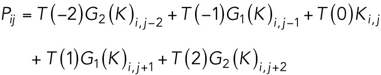
In the interest of computational efficiency, we truncated the length of our temporal kernel, T(n), to a size of 5 temporal pixels. We generated two Gaussian filter movies, one with a σ of 1 pixel for pixels in adjacent frames to pixel i which we denote as G₁(K) and one with a σ of 2 pixels for pixels 2 frames before and after pixel i which we denote as G₂(K). We chose a spatiotemporal window blur of 5 frames (2 frames before and after) since >95% of the moving motor signal in our data are maintained within 2 adjacent pixels. For every pixel i at frame j the estimated motion model 〈P〉 mean as:

4

For this work, all of our convolution operations use reflective boundary conditions. Each pixel in each frame of the resulting motion movie was temporally and spatially averaged with neighboring pixels; the resulting movie was more blurred than the calibrated movie, but maintained the signal from moving motors and background (Table 1; Figure 1C, Motion; and Supplemental Videos S1–S4).

Estimating stationary model 〈Q〉

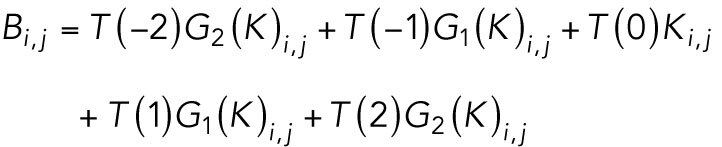
The program next generates a stationary model 〈Q〉 to represent the background fluorescence. The background within our data is structured and nonuniform, and Cega is suited for suppressing this fluctuating and structured background. The effectiveness of Cega is reliant on how well the stationary model estimates the background of the motion model. Since we used a sequence of expanding Gaussian filters to estimate 〈P〉, a similar level of blurring is required for the estimate of 〈Q〉, or there will be structural artifacts wherever the background has sharp features. To ensure 〈Q〉 has the same resolution as 〈P〉, we generate an intermediate movie of convolved filters without temporal correlations.

5

The temporal median filter was then applied to every pixel in B. This step is similar to the implementation of median filters for detecting fluorophore signals in single molecule localization microscopy data (Piccardi, 2004; Hoogendoorn et al., 2014), except with an added Gaussian filter. Ideally, the median filter needs to suppress dynamical fluctuations from moving motors while representing a gradually fluctuating background as accurately as possible. Therefore, the sliding window must exceed the duration of the moving motor signal, or else the motor signal will remain within the stationary model and will be removed when the Kullback-Leibler (KL) divergence is applied against the motion model. We chose a sliding window of 31 frames, 15 frames before and after the pixel of interest to sample our median pixel as it appeared to provide the best compromise between dynamics suppression and background estimation accuracy (Supplemental Figures S1 and S2). For our data, >95% of moving motors moved within this 31 frame range. The stationary model (Table 1; Figure 1C, Motion and Stationary; and Supplemental Videos S1–S4) used more frames than the motion model, and the resulting stationary movie is even more blurred than the motion movie. 〈Q〉 is defined as the movie generated after applying a nontemporal averaging of the Gaussian filters used on 〈P〉, followed by a temporal median filter with a sliding window of 31 frames.

KL divergence: segmenting moving particles from noisy data

Next, the differences between moving 〈P〉 and stationary 〈Q〉 models are used to resolve moving particles from stationary noise. To do so, we used the KL divergence (Kullback and Leibler, 1951) to estimate the dissimilarity between the stationary and the motion models. The general approach is to estimate two separate model hypotheses from the movie K and apply the KL divergence on a per-pixel basis that calculated the dissimilarity between groups.

The KL divergence for some random quantity x given hypothesis P and tested against null hypothesis Q is defined as:

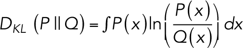6

In our application, we posited two hypotheses with Poisson statistics, the motion 〈P〉 and stationary 〈Q〉 models, where the quantity x represents the effective photon counts that could be measured in an image pixel. We hypothesized that the movie K is a single instance of x, a Poisson-like realization of the per pixel distribution P. We wanted to see how poorly a per pixel distribution Q would predict K if P more accurately modeled the input data and Q only modeled stationary objects. In other words, the pixels in either 〈P〉 or 〈Q〉 can be used to represent the expectation value of the pixels in K, but since they are different models they will lead to different probability densities per pixel. Since K is Poisson-like, this means that the KL divergence of the i-th pixel in Q from the i-th pixel in P is the KL divergence between two Poisson distributions:

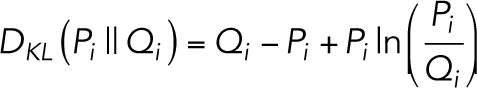7

Given estimators for 〈P〉 and 〈Q〉, the KL divergence movie (KLM) is generated (Table 1, Figure 1C, KL divergence; and Supplemental Videos S1–S4). The KL divergence model attenuated the background signal while enhancing the signal of moving motors, hence isolating the particles of interest over the background.

Connectivity filtering: denoising the KLM

The KLM has larger pixel values where the two models are in disagreement, suggesting evidence of mobile motors since 〈Q〉 was designed to ignore motion. However, the estimators are not perfect, and this results in unusually noisy pixels throughout the movie where 〈P〉 and 〈Q〉 are in spurious disagreement with one another. This produces white pixels, known as salt noise, that are sprinkled in throughout the movie, without producing darker pixels, or pepper noise. Since the data are under sampling the Nyquist limit, the additional effect of temporal averaging in 〈P〉 all but guarantees that the signal left by the moving motors spreads over multiple pixels. The spurious noise of the KLM is removed with a connectivity filter (Table 1; Figure 1C, Connectivity; and Supplemental Videos S1–S4), which eliminates all but the top 95% of the data within this model that includes the moving motor signal (Supplemental Figures S1 and S2). To do this, any 3 × 3 pixel subregion in the KLM must have at least 3 pixel values greater than the 95th quantile, measured to be 0.1 nats (units of natural logarithm), or the center pixel of that subregion is set to 0 in the connectivity movie. The remaining signal represented moving particles (colored circles in the connectivity row; Figure 1C and Supplemental Videos S1–S4).

LoG filtering and detecting local minima

The denoised KLM is then passed through a scale space Laplacian of Gaussian (LoG) filter (Lindeberg, 1998) to detect the local curvature of the signal left from the connectivity filter, using two σ values, 1 and 1.5 pixels, representing the parameter width of the filtering kernels (Table 1, Figure 1C, LoG; and Supplemental Videos S1–S4). This step enhanced the boundaries of the motors where there is a high transition from dark to bright signal and returned negative values at their peaks, which is why the signal appears as circles with black centers (colored circles in LoG row; Figure 1C). The smaller σ value represents a typical motor signal and the larger σ value helps to identify potential motors that are moving much faster and display a smeared information signature in the denoised KLM. We did not notice an improvement in object detection with additional scales in the LoG filter. Other SPT programs such as u-track (Jaqaman et al., 2008) and TrackMate (Tinevez et al., 2017) also use filters based on LoG segmentation, but apply them to raw data.

Local minima from the LoG filtered movies are then aggregated into a list of potential signal coordinates (Table 1, LoG Filter). The coordinates for each local minimum in LoG space (x, y, t) are used to retrieve the KL divergence score of the associated extremum pixel. Coordinates that point to a 3 × 3 region of KL divergence values that sum to less than a user-specified threshold were discarded. We used the 95th quantile of the connectivity movie (5 nats) to preserve only coordinate positions of moving motors (Supplemental Figures S1 and S2). After detection, coordinates can be connected into trajectories and analyzed with conventional tracking algorithms available for downstream SPT processing (Supplemental Videos S5–S8).

Movie S5.

Download video file ^{(22.6MB, mov)}

Detected particles using Cega for each processing step of axonal movie. Movies are displayed from top to bottom as follows: original movie, calibrated movie, stationary movie, motion movie, KL divergence movie, connectivity filter movie, LoG movie, track movie with LoG movie overlay, cumulative track movie. All movies except the last consist of the original movie with red or green boxes added to indicate locations of detected particles. Red boxes indicate locations of detected particles for each filtering step, while overlaid green boxes indicate particle positions detected after LoG filtering with Cega. The track movie overlaid on the LoG movie shows tracks detected within the last 5 frames, while the cumulative track movie indicates all tracks detected up until the current frame. Cyan colored tracks indicate particles moving to the anterograde (left) direction, while magenta colored tracks indicate those moving in the retrograde (right) direction. Movie set to play 10 fps, and scale bar set at 10 μm.

Movie S6.

Download video file ^{(2.4MB, mov)}

Zoom-in of Video 5. Movie set to play 10 fps, and scale bar set at 2 μm.

Movie S7.

Download video file ^{(21.7MB, mov)}

Detected particles using Cega for each processing step of dendritic movie. Movies are displayed from top to bottom as follows: original movie, calibrated movie, stationary movie, motion movie, KL divergence movie, connectivity filter movie, LoG movie, track movie with LoG movie overlay, cumulative track movie. All movies except the last consist of the original movie with red or green boxes added to indicate locations of detected particles. Red boxes indicate locations of detected particles for each filtering step, while overlaid green boxes indicate particle positions detected after LoG filtering with Cega. The track movie overlaid on the LoG movie shows tracks detected within the last 5 frames, while the cumulative track movie indicates all tracks detected up until the current frame. Cyan colored tracks indicate particles moving to the anterograde (left) direction, while magenta colored tracks indicate those moving in the retrograde (right) direction. Movie set to play 10 fps, and scale bar set at 10 μm.

Movie S8.

Download video file ^{(2.5MB, mov)}

Zoom-in of Video 7. Movie set to play 10 fps, and scale bar set at 2 μm.

COMPARISON TO EXISTING METHODS

Candidate finding

To test Cega’s ability to correctly detect simulated particles over typical background signal, we generated a time series of simulated particles by adding simulated photons on temporally filtered experimental data (see simulation methods). Fluorescent particles that represent GFP-K560 were simulated with mean photon emissions ranging from 50 to 600 photons per full frame of acquisition, corresponding to a signal-to-noise ratio (SNR) ranging from 0.7 to 8.5. This range includes the SNR within our experimental data (Wang et al., 2014), which was measured to be ∼4 following integration time, but also encompasses SNR expected from dimmer fluorescent proteins as well as brighter organic dyes. Moving particles were detected using Cega and background subtraction of median or minimum temporal filters with a 31 frame window, or standard particle detection with no background subtraction (Lindeberg, 1998). All methods were manually tuned with thresholds to maximize performance at a specific probe intensity. The background intensity was held fixed in simulations because detection capability is a function of SNR, and our simulations cover a large range of SNRs. The spot-finding algorithms had a threshold based on the maximum pixel value in a 3 × 3 pixel neighborhood of the estimated spot center. To quantitatively compare Cega’s performance against other particle detection methods processes, we calculated the Jaccard index and recall rate (see Materials and Methods). The Jaccard index is a statistic used to understand the similarities between sample sets (Milligan, 1981) and in this case is a measure related to the similarity between spot positions detected by each of the detection processes compared with the actual simulated spot positions. The recall rate, or true positive rate (TPR), is a measure of the ability of each of the detection processes to find all the simulated spots.

The performance of Cega was ranked among typical spot-finding algorithms that use the raw movie or a background-subtracted movie as the signal prior to scale space LoG filtering (Figure 2). No algorithm tested was capable of providing a detection solution at a SNR of ∼0.7, but Cega showed noticeable improvements at a SNR of ∼1.4 and the median background-subtracted spot finder matched performance after the SNR exceeded 4.2, which is greater than the range of our experimental data. The minimum background-subtracted spot finder met up with the prior two algorithms at a SNR of 4.9. The standard spot finder did not catch up in performance but started to improve significantly after the SNR exceeded 4.9.

FIGURE 2:

Analysis of Cega spot detection. (A, B) Jaccard index values calculated for simulated spots detected with Cega, median or minimum background subtraction methods, or standard methods, as the SNR increases. (C, D) Recall rate for detection methods as SNR increases. Simulations were run 100 times and resulted in a SD of <0.0045.

The trends from the Jaccard index test show that any sort of background subtraction is a vast improvement over spot finding with the raw image (Figure 2, A and B). The trends also show that Cega is able to discern between false signal and a moving motor with less information than the background-subtracted methods. The recall rate was high for all methods at high probe intensities but was at 50% for Cega at ∼0.7 SNR (Figure 2, C and D), since Cega could not reliably extract particle features at this SNR. The other methods, which had twice the recall rate at ∼0.7 SNR, had similar or lower Jaccard indices, which meant they had twice as many false positives. Finer parameter tuning could raise or lower Jaccard indices by a few percentage points, but the trends are clear: Cega performs more reliably at lower probe intensities and background subtraction methods converge in performance shortly thereafter.

In addition, receiver operating characteristics (ROC) curves indicate clearly that Cega outperforms the other spot-finding algorithms over a range of parameter values (Supplemental Figure S3). These curves, similar to Reismann et al. (2018), plot the TPR against the false detection rate (FDR) as one parameter is varied at a time. Points falling in the upper-left quadrant are ideal, as they maximize the number of true positives and limit the number of false positives. For Cega, we varied the stationary model sliding window size and the connectivity filter and LoG filter KLM thresholds. For the other spot-finding algorithms, we could only vary the pixel threshold. In general, the ROC curves resulting from sweeping Cega’s parameters were shifted to the left of that produced from sweeping the other spot-finding algorithms, suggesting that Cega did not produce as many false positives as the other detection methods over a large range of Cega’s parameter values. The values for the sliding window and connectivity filter and LoG filter KLM thresholds chosen for Cega detection fell well below a FDR of 0.5, where the true positive fits overpower the number of false-positive fits.

Tracking

We also tested the ability of Cega to effectively discard stationary particles, which becomes apparent when performing a full tracking experiment. Cega detection was performed on simulated data with mean photon emissions of 200, or 2.8 SNR, as this SNR is similar to that of the dimmer particles within our experimental data. After candidate finding, simulated motor spot coordinates were connected into trajectories using an in-house tracking software (Relich, 2016; Schwartz et al., 2017) based on the linear assignment problem (LAP) used in u-track (Jaqaman et al., 2008). The trajectories formed after application of Cega or median background subtraction were then displayed on kymographs and compared against the known simulated spot trajectories. Kymograph plots of simulated tracks show that parameter values chosen for Cega were optimal (Supplemental Figures S1 and S2), and spot detection using Cega provided for more accurate tracking of simulated particles compared with median background subtraction which had lower Jaccard indices (Figure 3). The zoom-in overlap shows that the median background subtraction methods resulted in many false tracks, most likely due to capturing background signal. Comparison of the Jaccard index and recall rates showed that Cega was more accurate in generating known tracks. This was true for simulated movies from both axons and dendrites with differing background signal. The difference in Jaccard index between tracks resulting from Cega and median background subtraction was greatest for the simulated axonal movie which contained uneven illumination and more background signal than the dendritic movie. In addition, Cega allowed for improved tracking in the simulated dendrite movie, where particle density was higher.

FIGURE 3:

Analysis of tracking after Cega or median background subtraction methods. Simulated data using axonal background signal was used where mean photon emissions were set to 200 photons, which corresponds to a SNR of 2.8. (A, B) Kymographs of tracks determined from simulated particles within axonal and dendritic compartments. Although the same number of particles were simulated in the axonal and dendritic movies, the dendritic movie was smaller in size, resulting in a higher density of particles. In the merge kymograph and zoom-in area, cyan indicates locations where only simulated tracks and Cega detected tracks overlap, whereas yellow indicates where only simulated tracks and median background-subtracted detected tracks overlap. Magenta tracks are where only Cega and median background-subtracted tracks overlap. Jaccard indices and recall rates for tracks determined after Cega filtering and median background subtraction are listed below each corresponding kymograph.

After testing Cega with simulated data, we used Cega to analyze our experimental data (Figure 4). Motor tracks detected during Cega analysis of experimental movies were mostly linear, with velocities similar to those expected from kinesin-1 motors in an in vitro system, while median background subtraction produced many tracks containing spurious noise, resulting in nonuniform tracks. We also found that Cega was able to track motors that switched direction during movement (Figure 4B, zoom-in). As these directional switches were not detected in this data set with programs such as u-track (Jaqaman et al., 2008) and TrackMate (Tinevez et al., 2017), the Cega algorithm provides a more reliable analysis of the data from these complex microtubule arrays.

FIGURE 4:

Analysis of Cega performance on original data set. (A, B) Kymographs of tracks determined from kinesin motors moving on microtubule arrays within axonal and dendritic compartments. In the merge kymograph, yellow areas indicate where Cega and median background-subtracted detected tracks overlap.

DISCUSSION

SPT software allows automated quantitative analysis of both in vitro and in vivo experimental data. However, as experimental systems become more complex, background signal often increases and becomes nonuniform, posing a significant challenge to current software. As an example, we analyzed the motility of kinesin motors moving along extracted neuronal cytoskeletal arrays, as these data are much noisier than data from more reductionist single molecule in vitro assays and contain spatially and temporally varying background. The quantitative metrics and qualitative comparisons shown here make it clear that more sophisticated particle identification methods are required to reliably extract SPT information from more complex data sets. Conventional spot-finding algorithms use pixel intensity metrics for thresholding of real signals from artifacts. In our data sets from motility along extracted neurons, intensity-based metrics failed to reliably threshold real motor signals from noise. As a result, more than half of the trajectories recovered from SPT software were false. Cega, on the other hand, uses statistical calculations which factor in background estimations so that artifacts from local regions of high background fluorescence are mitigated. Use of Cega on experimental data resulted in a dramatic reduction and temporal shortening of false trajectories.

We found that Cega was dependent on the quality of the background estimation technique used to determine 〈Q〉. Before settling on a temporal median background estimator, we first tried using the temporal minimum filter, but we found that the median filter was a better discriminator of signal over noise at lower photon counts. It is possible that there is an ideal quantile value for background estimation, but it was not an avenue we explored because it seemed that finding the optimal quantile would be dependent on specific experimental conditions. Another avenue for optimization would be to incorporate a weighted spatiotemporal median filter instead of the standard temporal median filter (Brownrigg, 1984). The current implementation of Cega outperforms current background subtraction methods when analyzing neuronal data sets. Still, we believe that further improvement of Cega is feasible and future studies should focus on improving the accuracy of background estimation. For example, more accurate background estimation techniques utilizing deep learning have been developed recently (Möckl et al., 2020) and incorporating these into the estimation of 〈Q〉 could improve the KLM movie.

The Jaccard index and the recall rate from a range of detection techniques that were compared demonstrate that Cega had better performance than a typical spot finder with background-subtracted data (Hoogendoorn et al., 2014). In either instance, the recall rate of both methods could approach 100%, but the number of false positives would skyrocket; this information on spot reliability is conveyed by the Jaccard index. Unfortunately, the Jaccard index does not fully represent tracking capability, as a false negative compromises tracking software much more than a false positive (Smal and Meijering, 2015), but this is only true when false positives are not spatiotemporally correlated to one another. We treat the Jaccard index as a baseline for the potential of a successful tracking analysis. A Jaccard index over 0.9 is very likely to return accurate, full-length trajectories. A Jaccard index of 0.5 is more likely to return partial trajectories if the recall rate is low or is more likely to return a high percentage of false trajectories if the recall rate is high and the artifacts are correlated. Therefore, although the Jaccard index and recall rate alone are not sufficient to guarantee tracking performance, together they provide good indicators as to assess the relative quality of tracking algorithms.

Our simulations were designed to be optimal for particle detection against structured background signal from our data sets. The simulations were generated by adding photons from simulated motors on a median background estimate of axonal and dendritic movies. The median background was taken from a much shorter temporal window (7 frames) than what is used from our spot-finding analyses (31 frames). The reason for this was that a shorter temporal median filter preserved the background structure better. Legitimate motors from experimental data were not completely filtered out as a direct consequence of using a shorter temporal window in the median filtering of our simulated data. As a result, there were spatiotemporally correlated pixels that highlight moving particles in our background data. The estimation artifacts guaranteed that none of the measured spot-finding algorithms could score a perfect Jaccard index of 1. The moving background artifacts resulted in a few spurious particle coordinates in Figure 2 which actually corresponded to true trajectories in Figure 3. Nevertheless, all spot-finding algorithms we tested tracked these artifacts. While the parameters that we used here were optimal for tracking moving motors, Cega is capable of detecting motors that intermittently pause as long as a window size encompassing the duration of >95% of the particles of interest is chosen for the stationary model estimation.

SPT remains an open problem and the field is constantly evolving. For this work, we used a consistent tracking software so we could focus on assessing the quality of the initial spot detection algorithm chosen. The in-house tracking software used here (Relich, 2016; Schwartz et al., 2017), based on the LAP used in u-track (Jaqaman et al., 2008), in combination with Cega, allowed for tracking of moving motors within a dense background. Importantly, Cega spot detection allowed for the tracking of motors that change directions, something that programs such as u-track (Jaqaman et al., 2008) and TrackMate (Tinevez et al., 2017) were unable to accomplish with this experimental data set. However, the tracking software we used is still not optimal for this problem; aside from the spot candidates, the additional information generated from Cega is not incorporated into the downstream tracking algorithms. Incorporating the heterogeneous background information or the KL divergence score into downstream tracking methods would increase the robustness of the tracker in noisier data. Most notably is the localization algorithm used in this study. Our chosen tracker has a localization algorithm incorporating MAPPEL software (Olah, 2019), which does not incorporate the estimated background information from Cega. As a result, the returned fit statistics are suboptimal indicators for the tracking phase. It is well known that incorporating prior background information greatly enhances the accuracy and recall rate of single molecule microscopy (Hoogendoorn et al., 2014), so measuring the trajectory improvements from an enhanced localization estimator would be a good next step in improving tracking resources for motors community.

Although there are many components in SPT that are yet to be refined for tracking in more complex data sets such as the neuronal data analyzed here, Cega presents a marked improvement in a critical component of the greater SPT workflow. By using statistical hypothesis techniques to segment background, we were able to track moving particles more reliably while discarding nuisance objects. Our refined trajectories dramatically minimize false trajectories because Cega is a better discriminator of signal than intensity-based, spot-finding algorithms. By estimating a baseline of accuracy in the beginning phases of a tracking algorithm, we can dramatically improve downstream performance for all SPT algorithms that are structured to identify particles before the connecting trajectories.

MATERIALS AND METHODS

Protein expression and purification

K560-GFP protein was purified as described in (McIntosh et al., 2018) with the following modifications. The K560-GFP DNA was transformed into BL21(DE3)pLysE bacteria (Sigma Aldrich, CMC0015-20 × 40UL) and cultures containing the plasmid were grown at 37°C until an OD600 of 0.4 was reached. Protein expression was then induced with 0.15 mM IPTG for 18 h at 18°C. Cells were pelleted and flash frozen in liquid nitrogen and stored at –80°C. On the day of purification, cells were resuspended in lysis buffer (50 mM NaPO₄, 250 mM NaCl, 20 mM Imidazole, 1 mM MgCl₂, 0.5 mM ATP, 1 mM β-ME, 0.01 mg/ml aprotinin and leupeptin, pH 6.0) and lysed by passage through a microfluidizer (Microfluidics). Lysate was clarified by centrifugation at 42,000 rpm for 30 min and subsequently run over a Co₂₊ agarose bead (GoldBio, H-310-25) column at 1 ml/min. Bound protein was washed with wash buffer (50 mM NaPO₄, 300 mM NaCl, 10 mM Imidazole, 1 mM MgCl₂, 0.1 mM ATP, 0.01 mg/ml aprotinin and leupeptin, pH 7.4) and eluted with elution buffer (50 mM NaPO₄, 300 mM NaCl, 150 mM Imidazole, 1 mM MgCl₂, 0.1 mM ATP, pH 7.4). Elution fractions were pooled and concentrated. Buffer was exchanged to BRB80 (80 mM NaPIPES, 1 mM MgCl₂, 1 mM EGTA, pH 6.8) by loading protein over Nap10 (GE Healthcare, 17-0854-01) and PD10 (GE Healthcare, 17-0851-01) exchange columns. MT affinity/dead-head spin was performed as described in (McIntosh et al., 2018). Protein concentration was determined using Pierce BCA Protein Assay Kit (ThermoFischer Scientific, 23225).

Neuronal cell culture

Thirty-five millimeter glass-bottom dishes (MatTek, P35G-1.5-14-C) were coated with 0.5 mg/ml poly-l-lysine (Sigma-Aldrich, P1274) overnight and rinsed with dH₂0 and MEM (Life Technologies, 1109-072) prior to plating neurons. E18 Sprague–Dawley rat hippocampal neurons were received from the Neuron Culture Service Center at the University of Pennsylvania and plated in attachment media (MEM [Life Technologies, 1109-072] supplemented with 10% horse serum [Life Technologies, 26050-070], 33 mM glucose [Corning, 25-037-CIR], and 1 mM sodium pyruvate [Life Technologies, 11360-070]) at a density of 250,000 cells per dish and cultured 37°C with 5% CO₂. After 4–6 h of attachment, media were replaced with maintenance media (Neurobasal [Life Technologies, 21103-049] supplemented with 33 mM glucose [Corning, 25-037-CIR], 2 mM GlutaMAX [Life Technologies, 35050-061], 100 units/ml penicillin, 100 µg/ml streptomycin [Life Technologies, 15140-122], and 2% B27 [Life Technologies, 17504-044]);. 24 h after initial plating, AraC (Sigma Aldrich, C6645) was added at 10 µM to prevent glial cell division.

Motor-PAINT assay

The neuronal MT cytoskeleton was extracted, stabilized, and fixed according to previous work (Tas et al., 2017) with slight modifications. At 9-10 DIV, membranes were extracted from neurons by incubation with extraction buffer (1 M sucrose, 0.15% Triton-X in BRB80, pH 6.8, at 37°C) for 1 min. An equal amount of fixation buffer (1% paraformaldehyde in BRB80, pH 6.8, at 37°C) was added for 1 min with gentle swirling. Dishes were rinsed 3× with wash buffer (2 µM Paclitaxel in BRB80, pH 6.8, at 37°C) and once more right before imaging. For imaging, extracted MT arrays were placed in imaging buffer (1 mM ATP, 2 µM Paclitaxel, 0.133 mg/ml casein [Sigma Aldrich, C5890-500G], 0.133 mg/ml bovine serum albumin [Fischer Scientific, 50-253-90], 4 mM DTT, 6 mg/ml glucose, 49 U/ml glucose oxidase [Sigma, G2133-250KU], 115 U/mg catalase [Sigma, C100-500MG], 0.21 mg/ml creatine phosphokinase [Sigma, C3755-35KU], and 4.76 mM phosphocreatine [Sigma, P7936-1G] in BRB80, pH 6.8) containing 5–10 nM K560-GFP motor dimer.

Microscopy

Motor-PAINT assays were performed at 37°C using a PerkinElmer Nikon Eclipse Ti TIRF system using a Nikon Apo TIRF 100 × 1.49 NA oil-immersion objective and a Hamamatsu ImagEM C9100-13 EMCCD camera operated by Volocity software. Movies were obtained by continuously acquiring K560 motor images at 5 fps for 2 min.

Offset and gain calibration

Gain calibration of the Hamamatsu ImagEM C9100-13 EMCCD camera was performed by fusing techniques from standard and automated gain calibration practices. Our camera had a few damaged pixels in the upper-right quadrant of the sensor region of interest (ROI). The damaged pixels caused errors in automated gain calibration (Heintzmann et al., 2018), but we were able to reliably track molecules with scalar gain, offset, and read noise variance parameters by cropping the sensor ROI so that only undamaged pixels were used in the following gain regression algorithms.

First, a dark movie was acquired with 200 frames with the camera shutter closed. The mean pixel value of the dark movie used the estimate for O and the corresponding variance was the estimate for var(R) in units of ADU².

We performed the single shot gain estimator on a few cropped images given knowledge of O and var(R) and we extracted an averaged G as our gain parameter using the single shot gain estimation algorithm described in Heintzmann et al. (2018). With G we were able to determine that var(R) G^–2 << 1 on this camera which allowed us to ignore the effects of additive read noise for the remainder of our analysis. The technique failed when processing with the complete camera ROI because a strip of about 6 adjacent camera pixels that appeared to have been damaged by a photon oversaturation event resulted in an overestimation of the energy contribution from the high frequency Fourier spectrum. The damaged pixels were noticeably darker than the more functional neighboring pixels, but they were spatially correlated, limited in number, and did not noticeably affect tracking results or biological experiments.

We estimated our Poisson movie K ≈ (S–O)G^–1 and discarded the read noise term. We use the movie K for all of our subsequent analysis for Cega and downstream tracking.

Motor protein simulations

Simulated data were generated by fusing a background estimate of experimental data with simulated photon signatures from procedurally generated trajectories. The resulting process provided a realistic movie with simulated motor photons and a ground truth of averaged positions.

The experimental movie was stripped of its true motor proteins via a median filter with a temporal width of 7 frames. The shortened temporal median filter provided a more accurate depiction of the experimental background data but left some noticeable residual emissions from moving motors wherever the motors had aggregated. This resulted in data where a certain fraction of false positives was guaranteed with experimentally relevant photon intensities for the simulated motors. Poisson noise was added to the median filtered movie.

The motor photon trajectory positions were calculated at time points before and after every simulated camera acquisition. The rough positions were modeled from a Kalman filter process, where proteins are subjected to diffusion with drift, but a white process noise is applied to the drift velocity so that proteins could gradually change direction and speed. The initial mean velocities were drawn from a log normal distribution to match the distribution of velocities observed in experimental data. Motor protein photons were painted by interpolating discrete trajectory positions with a Brownian bridge (Lindén et al., 2016) given exponentially sampled time points with a rate set by the mean photon parameter.

The final simulation movie consists of the simulated motor photons, summed with the background movie and white noise. The white noise had a σ of 0.1 photons that was added to all pixels to simulate extra read noise.

SNR

We calculated the SNR for data of simulated motors with mean photon emissions ranging from 50 to 600 photons per full frame of acquisition based on the following equation described in Salehi-Reyhani (2017):

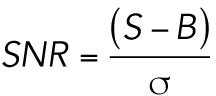8

where S is the maximal peak intensity of the simulated molecules, B is the average background pixel intensity, and σ is the SD of the background pixel intensity.

Jaccard index score and recall rate

The Jaccard index (Milligan, 1981) is an algorithm performance metric defined as:

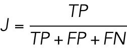9

where TP is the number of true positives, FP is the number of false positives, and FN is the number of false negatives when comparing a list of coordinates to a known ground truth. Similarly, the recall rate is defined as:

10

and is useful for determining how well a true trajectory can be reconstructed if there was a downstream method for removing false positives.

To score the performance of Cega and the other spot finders, the LAP (Jonker and Volgenant, 1987) was used to assign the nearest true coordinates to the algorithm coordinates. The squared distance between ground truth and algorithm coordinates plus 1 was used as the cost for assignment. The birth and death costs were set to 4. Any assignment costs greater than 4 were discarded to prevent assigning coordinate pairs that were separated by at least 2 pixels. Coordinate pairs that were assigned to one another were counted as true positives, true coordinates did not pair were scored as false negatives, and algorithm coordinates that did not pair were scored as false positives. For trajectories formed after spot detection with Cega and the other spot finders, the Jaccard index and recall rates were calculated by taking each kymograph and measuring the overlap of track segments to the ground truth on a pixel basis.

Tracking software

The tracking software implemented for this paper was adapted from the MATLAB software developed for Relich (2016) and Schwartz et al. (2017) and is based on the software used in u-track (Jaqaman et al., 2008). A few minor modifications were applied to make the workflow amenable to motor proteins, primarily the blob-finding routine for initial candidate selection was replaced with Cega. The software in its current implementation does not yet incorporate heterogeneous background information in the localization routines. A median background subtraction on the data was considered for the localization routine but was omitted from this exposition because the maximum a posteriori estimator cannot process negative pixel values. The same tracking software and parameters were used for all comparisons between Cega and the median-subtracted spot finder.

Abbreviations used:

ADU

arbitrary digital unit

FDR

false detection rate

fps

frames per second

KL

Kullback-Leibler

KLM

KL divergence movie

LAP

linear assignment problem

LoG

Laplacian of Gaussian

nats

units of natural logarithm

ROC

receiver operating characteristics

ROI

region of interest

SNR

signal-to-noise ratio

SPT

single particle tracking

TIRF

total internal reflection fluorescence

TPR

true positive rate.

REFERENCES

- Babcock HP, Huang F, Speer CM (2019). Correcting artifacts in single molecule localization microscopy analysis arising from pixel quantum efficiency differences in sCMOS cameras. Sci Rep 9, 18058. [DOI] [PMC free article] [PubMed] [Google Scholar]
- Belyy V, Yildiz A (2014). Processive cytoskeletal motors studied with single-molecule fluorescence techniques. FEBS Lett 588, 3520–3525. [DOI] [PMC free article] [PubMed] [Google Scholar]
- Brownrigg D (1984). The weighted median filter. CACM. https//.org/10.1145/358198.358222 [Google Scholar]
- Chenouard N, Dufour A, Olivo-Marin J-C (2009). Tracking algorithms chase down pathogens. Biotechnol J 4, 838–845. [DOI] [PubMed] [Google Scholar]
- Heintzmann R, Relich PK, Nieuwenhuizen RPJ, Lidke KA, Rieger B (2018). Calibrating photon counts from a single image. ArXiv Preprint http://arxiv.org/abs/1611.05654.
- Hoogendoorn E, Crosby KC, Leyton-Puig D, Breedijk RMP, Jalink K, Gadella TWJ, Postma M (2014). The fidelity of stochastic single-molecule super-resolution reconstructions critically depends upon robust background estimation. Sci Rep 4. https//.org/10.1038/srep03854. [DOI] [PMC free article] [PubMed] [Google Scholar]
- Huang F, Hartwich TMP, Rivera-Molina FE, Lin Y, Duim WC, Long JJ, Uchil PD, Myers JR, Baird MA, Mothes W, et al. (2013). Video-rate nanoscopy using sCMOS camera-specific single-molecule localization algorithms. Nat Methods 10, 653–658. [DOI] [PMC free article] [PubMed] [Google Scholar]
- Jaqaman K, Loerke D, Mettlen M, Kuwata H, Grinstein S, Schmid SL, Danuser G (2008). Robust single-particle tracking in live-cell time-lapse sequences. Nat Methods 5, 695–702. [DOI] [PMC free article] [PubMed] [Google Scholar]
- Jonker R, Volgenant A (1987). A shortest augmenting path algorithm for dense and sparse linear assignment problems. Computing 38, 325–340. [Google Scholar]
- Kalaidzidis Y (2007). Intracellular objects tracking. Eur J Cell Biol 86, 569–578. [DOI] [PubMed] [Google Scholar]
- Kullback S, Leibler RA (1951). On Information and Sufficiency. Ann Math Stat 22, 79–86. [Google Scholar]
- Lindeberg T (1998). Feature detection with automatic scale selection. Int J Comput Vis 30, 79–116. [Google Scholar]
- Lindén M, Ćurić V, Boucharin A, Fange D, Elf J (2016). Simulated single molecule microscopy with SMeagol. Bioinformatics 32, 2394–2395. [DOI] [PMC free article] [PubMed] [Google Scholar]
- Mathiot M (1973). A Dictionary of Papago Usage, Indiana University. [Google Scholar]
- McIntosh BB, Pyrpassopoulos S, Holzbaur ELF, Ostap EM (2018). Opposing kinesin and Myosin-I motors drive membrane deformation and tubulation along engineered cytoskeletal networks. Curr Biol 28, 236–248.e5. [DOI] [PMC free article] [PubMed] [Google Scholar]
- Meijering E, Smal I, Danuser G (2006). Tracking in molecular bioimaging. IEEE Signal Process Mag 23, 46–53. [Google Scholar]
- Milligan GW (1981). A monte carlo study of thirty internal criterion measures for cluster analysis. Psychometrika 46, 187–199. [Google Scholar]
- Möckl L, Roy AR, Petrov PN, Moerner WE (2020). Accurate and rapid background estimation in single-molecule localization microscopy using the deep neural network BGnet. Proc Natl Acad Sci USA 117, 60–67. [DOI] [PMC free article] [PubMed] [Google Scholar]
- Mortensen KI, Churchman LS, Spudich JA, Flyvbjerg H (2010). Optimized localization analysis for single-molecule tracking and super-resolution microscopy. Nat Methods 7, 377–381. [DOI] [PMC free article] [PubMed] [Google Scholar]
- Mortensen KI, Flyvbjerg H (2016). “ Calibration-on-the-spot”: How to calibrate an EMCCD camera from its images. Sci Rep 6, 28680. [DOI] [PMC free article] [PubMed] [Google Scholar]
- Murphy DB, Davidson MW (2012). Digital image processing. In: Fundamentals of Light Microscopy and Electronic Imaging, 2nd ed., John Wiley & Sons, 415–449. [Google Scholar]
- Olah MJ (2019). Mappel [C++]. Retrieved from https://github.com/markjolah/Mappel (Original work published 2017)
- Piccardi M (2004). Background subtraction techniques: A review. 2004 IEEE International Conference on Systems, Man and Cybernetics (IEEE Cat. No.04CH37583), 4, 3099–3104. [Google Scholar]
- Pierce DW, Hom-Booher N, Vale RD (1997). Imaging individual green fluorescent proteins. Nature 388, 338. [DOI] [PubMed] [Google Scholar]
- Reismann AWAF, Atanasova L, Schrangl L, Zeilinger S, Schütz GJ (2018). Temporal filtering to improve single molecule identification in high background samples. Molecules 23, https//.org/10.3390/molecules23123338 [DOI] [PMC free article] [PubMed] [Google Scholar]
- Relich P (2016). Single Particle Tracking: Analysis Techniques for Live Cell Nanoscopy . https://digitalrepository.unm.edu/phyc_etds/142 [Google Scholar]
- Salehi-Reyhani A (2017). Evaluating single molecule detection methods for microarrays with high dynamic range for quantitative single cell analysis. Sci Rep 7, 17957. [DOI] [PMC free article] [PubMed] [Google Scholar]
- Schwartz SL, Cleyrat C, Olah MJ, Relich PK, Phillips GK, Hlavacek WS, Lidke KA, Wilson BS, Lidke DS (2017). Differential mast cell outcomes are sensitive to FcεRI-Syk binding kinetics. Mol Biol Cell 28, 3397–3414. [DOI] [PMC free article] [PubMed] [Google Scholar]
- Smal I, Meijering E (2015). Quantitative comparison of multiframe data association techniques for particle tracking in time-lapse fluorescence microscopy. Med Image Anal 24, 163–189. [DOI] [PubMed] [Google Scholar]
- Tas RP, Chazeau A, Cloin BMC, Lambers MLA, Hoogenraad CC, Kapitein LC (2017). Differentiation between oppositely oriented microtubules controls polarized neuronal transport. Neuron 96, 1264–1271.e5. [DOI] [PMC free article] [PubMed] [Google Scholar]
- Tinevez J-Y, Perry N, Schindelin J, Hoopes GM, Reynolds GD, Laplantine E, Bednarek SY, Shorte SL, Eliceiri KW (2017). TrackMate: An open and extensible platform for single-particle tracking. Methods 115, 80–90. [DOI] [PubMed] [Google Scholar]
- Vale RD, Funatsu T, Pierce DW, Romberg L, Harada Y, Yanagida T (1996). Direct observation of single kinesin molecules moving along microtubules. Nature 380, 451–453. [DOI] [PMC free article] [PubMed] [Google Scholar]
- Wang S, Moffitt JR, Dempsey GT, Xie XS, Zhuang X (2014). Characterization and development of photoactivatable fluorescent proteins for single-molecule-based superresolution imaging. Proc Natl Acad Sci USA 111, 8452–8457. [DOI] [PMC free article] [PubMed] [Google Scholar]
- Young IT, Gerbrands JJ, van Vliet LJ (1998). Fundamentals of Image Processing. Delft, Netherlands: Delft University of Technology. [Google Scholar]
Associated Data
This section collects any data citations, data availability statements, or supplementary materials included in this article.