Analysis of Proportional Data in Reproductive and Developmental Toxicity Studies: Comparison of Sensitivities of Logit Transformation, Arcsine Square Root Transformation, and Nonparametric Analysis

Abstract

Background

In developmental and reproductive toxicity studies, analysis of litter-based binary endpoints (e.g., incidence of malformed fetuses) is complex in that littermates often are not entirely independent of one another. It is well established that the litter, not the individual fetus, is the proper independent experimental unit in statistical analysis. Accordingly, analysis is often based on the proportion affected per litter and the litter proportions are analyzed as continuous data. Because these proportional data generally do not meet assumptions of symmetry or normality, data are typically analyzed by nonparametric methods, arcsine square root transformation, or logit transformation.

Methods

We conducted power calculations to compare different approaches (nonparametric, arcsine square root-transformed, logit-transformed, untransformed) for analyzing litter-based proportional data. A reproductive toxicity study with a control and one treated group provided data for two endpoints: prenatal loss, and fertility by in utero insemination (IUI). Type 1 error and power were estimated by 10,000 simulations based on two-sample one-tailed t-tests with varying numbers of litters per group. To further compare the different approaches, we conducted additional analyses with shifted mean proportions to produce illustrative scenarios.

Results

Analyses based on logit-transformed proportions had greater power than those based on untransformed or arcsine square root-transformed proportions, or nonparametric procedures.

Conclusion

The logit transformation is preferred to the other approaches considered when making inferences concerning litter-based proportional endpoints, particularly with skewed distributions. The improved performance of the logit transformation becomes increasingly pronounced as the response proportions are increasingly close to the boundaries of the parameter space.

INTRODUCTION

Binary data are the simplest type of statistical data, arising when there are just two possible outcomes, e.g., yes-no, success-failure, life-death, sick-healthy, etc. In developmental and reproductive toxicity studies, analysis of binary endpoints regarding pups, fetuses, or implantation sites (e.g., incidence of resorbed implantation sites, incidence of malformed fetuses, etc.) becomes more statistically complex in that offspring within a litter usually are not independent. Because intra-litter correlation (known as the “litter effect”) must be accounted for, it is well established that the litter, rather than the individual fetus or pup, is the proper independent experimental unit in statistical analysis (Chen, 2006). In developmental and reproductive toxicity studies, analysis of binary data is often based on the proportion affected per litter and the litter proportions are analyzed as continuous data. Because distributions of these proportional data generally do not meet assumptions of symmetry or normality required for parametric analysis such as analysis of variance (ANOVA), data may be ranked (i.e., for nonparametric analysis) or transformed to approximate normality (Glass et al., 1972). Nonparametric analysis (e.g., Kruskal-Wallis test or Wilcoxon Mann Whitney test) is a commonly used approach in the developmental toxicity literature; i.e., the untransformed proportions are ranked, and the ranks are then analyzed by ANOVA.

In the mid 1900’s the arcsine square root transformation was suggested (e.g., Snedecor & Cochran, 1967) for analyzing binomially distributed proportional data in toxicology and the environmental sciences since it is a normalizing and variance stabilizing transformation for binomially distributed data when the response proportion is removed from 0 or 1. However proportions based on binary data may be more variable than would be predicted by the binomial distribution. This would be the case if there are litter effects (i.e. litter-to-litter variation within control or treatment groups). In developmental toxicity studies, littermates are not entirely independent, which leads to correlated binary responses (and the strength of the correlation can vary from endpoint to endpoint).

Because of differences in litter sizes within treatment groups, the observed individual litter proportions are not identically distributed and this needs to be accounted for when analyzing the data after the experiment has been run (Chen, 2006). Chen suggests the use of a beta-binomial model (Williams, 1975) in which the responses within each litter are binomially distributed but the response probability varies from litter to litter according to a beta distribution. The parameters of the beta distribution vary among treatment groups. This results in a marginal model with a mean response probability p across litters within a group and variation among litters exhibiting variation greater than what would be predicted due solely to binomial variation.

An alternative approach at the analysis stage is mixed effects logistic regression in which the responses within each litter within a treatment group are modeled as binomially distributed with random response probability ρ. This permits the response probability to vary among litters within a treatment group, as noted above. Mixed effects logistic regression is used by the National Toxicology Program (NTP) for the analysis of multi-group binary data involving litter structures (e.g., NTP, 2012; Catlin et al., 2018). Jaeger (2008) also recommends the use of mixed effects logistic regression as a superior alternative to ANOVA to account for litter-to-litter variation and within-litter variation in one analysis model. He states that “…even after applying the arcsine square root transformation to proportional data, ANOVA can yield spurious results….”

The situation differs when power analyses are conducted for designing a future experiment. In the design of future studies, the litter sizes have not yet been attained and so litter sizes are unknown. A common assumption at the planning stage is that litter sizes will be constant within treatment groups (but may vary across groups). For planning purposes, it is usual statistical practice that litters are assumed to be independently and identically distributed within treatment groups. The assumed standard deviation among litters within treatment groups is based on that which was observed in previous data. Sometimes a covariate is incorporated into the models to reflect a continuous factor such as age, temperature, etc. It is also usual practice that except perhaps for the very smallest experiments, where small sample exact analysis methods are sometimes used, to analyze experimental results with large sample normal theory approximations to the distributions of the inference statistics, such as t-statistics, ANOVA and chi square statistics, and likelihood based tests and estimators. Small sample inference procedures, not based on asymptotic theory, exist such as jackknife and bootstrap methods (Efron, 1986). Such methods are much less commonly utilized by experimental contributors in the developmental toxicology literature than the normal theory based methods discussed above. They will not be considered further in this paper.

Here we use power analyses to explore the relative strengths and weaknesses of the different approaches to analyzing litter-based proportional data. I.e., approaches that yield the greatest power will likely be the approaches most able to detect differences between experimental groups when analyzing litter-based proportional data. The power analyses are based on empirical computer simulations assuming that t-test or Wilcoxon Mann Whitney normal approximation critical values are used for comparisons among groups (Agresti, 2012). The values of power presented are empirical.

Here, in the planning stages of a study to evaluate the reproductive toxicity of mixtures in rats, power calculations were conducted for several endpoints based on data from a previous study where the reproductive toxicity of a mixture of drinking water disinfection by-products (DBPs) was evaluated in rats (Narotsky et al., 2013). In that study, a treated group receiving a complex mixture of DBPs was compared against a control group receiving purified water. In this paper, analyses are carried out to compare the power to detect different effect sizes (i.e., the deviation between group mean proportions) using different data transformations based on the variability observed in Narotsky et al. (2013) and the numbers of litters per group to be tested. Two proportional endpoints are evaluated: prenatal loss and fertility by in utero insemination (IUI). Prenatal loss, a basic endpoint in reproductive and developmental toxicity studies, reflects the litter’s prenatal attrition from implantation to term. The other proportional endpoint, IUI fertility, is not commonly part of reproductive toxicity studies. Because male rats ejaculate an excess of qualitatively normal sperm, this assay provides increased sensitivity for detecting a decrease in sperm quality in the rat by using a fixed, critical number of sperm from control or treated males to inseminate receptive untreated females (Klinefelter, 2002).

METHODS

Data for the two proportional endpoints analyzed here, prenatal loss and IUI fertility, were obtained from Narotsky et al. (2013). Briefly, timed-pregnant Sprague-Dawley rats (P0 generation) received purified water (control group) or a chlorinated water concentrate (treated group) as drinking water during gestation and lactation. Exposure to the F1 offspring continued postweaning. Detailed information on the experimental design is provided in Narotsky et al. (2013). Prenatal loss for each litter is defined as the number of uterine implantation sites minus the number of F1 viable pups at postnatal day 0, divided by the number of implantation sites. Prenatal loss was calculated for 79 control and 118 treated F1 litters. For IUI fertility, 14 control and 15 treated F1 adult males were assessed by injecting epidydimal sperm into the uterine horns of untreated receptive females (1 female per male); corpora lutea (reflecting ovulations) and uterine implantation sites were counted 9 days post-insemination. The IUI fertility of the donor male is expressed as the proportion of implantation sites per corpora lutea.

In the situation considered in this paper, there is a control group and a treated group i = 0, 1, with population mean proportions p₀, p_1, and standard deviations among the litter proportions σ₀, σ₁. The unit of analysis is the litter proportion. The litter standard deviation includes both within litter (binomial) variation as well as litter-to-litter variation. Litter-to-litter variation in response proportions within groups is often modeled as beta distributed with means and standard deviations specified on historical data. This combination of variance components results in variation in excess of binomial distribution variation. Power analyses were carried out for IUI fertility and prenatal loss when analyzed with the following approaches: untransformed proportions, Wilcoxon Mann Whitney tests on the ranks of the untransformed proportions, arcsine square root-transformed proportions [arcsine(√p)], and logit-transformed proportions [ln(p/(1-p))].

Empirical Power Comparisons Based on Simulated Distributions of Proportions and Their Logit and Arcsine Square Root Transformations

To illustrate empirically through simulation the characteristics of the distributions of litter proportions and inferences based on them, it was assumed that the individual litter proportions (untransformed) were drawn from beta distributions with the means and standard deviations shown in Table 1 (original data). At the analysis stage, after the data have been collected, the response proportions in individual litters within treatment groups will have binomial distributions, with litter means varying randomly across litters, and with group means p₀ and p₁ and group standard deviations σ₀ and σ₁ across litters. The average response across litters is asymptotically normally distributed (based on the Central Limit Theorem) (Feller, 1966) with mean p and standard deviation σ. At the planning stage, before the data have been collected, the litter sizes are unknown, and it is a common planning assumption that the individual litters are independently and identically distributed within treatment groups. Because the beta binomial distribution and the beta distribution are both distributions in the interval (0,1), with the same mean and standard deviation, and because the average distributions across litters are asymptotically the same (normal), the simulated beta distribution response averages can be used to carry out power comparisons between the treatment and control groups. The beta distribution is a two-parameter distribution on the variable x varying in the interval (0, 1) with parameters α > 0, β > 0. The probability density function of the beta (α, β) distribution is

$$\frac{\mathrm{\Gamma }(\mathbf{\alpha }+\mathbf{\beta )}}{\mathbf{\Gamma (\alpha )\Gamma (\beta })}{x}^{\alpha -1}{(1-x)}^{\beta -1}\mathbf{\hspace{0.17em}}\mathbf{\hspace{1em}}0<x<1,\mathrm{\alpha }>0,\mathrm{\beta }>0$$

where Γ(·) is the mathematical gamma function (Casella & Berger, 2002). There is a one-to-one mathematical correspondence (NIST/SEMATECH, 2012) between the beta distribution parameters (α, β) and the means p and standard deviations σ shown in Table 1. Namely

$$\mathbf{\alpha }\mathbf{\hspace{0.17em}}=\mathbf{\hspace{0.17em}}\left(\frac{\mathbf{p(1}\mathbf{\hspace{0.17em}}-\mathbf{p)}\mathbf{\hspace{0.17em}}-\mathbf{\hspace{0.17em}}{\mathbf{\sigma }}^{\mathbf{2}}}{{\mathbf{\sigma }}^{\mathbf{2}}}\right)\mathbf{p},\mathbf{\beta }=\left(\frac{\mathbf{p(1}\mathbf{\hspace{0.17em}}-\mathbf{p)}\mathbf{\hspace{0.17em}}-\mathbf{\hspace{0.17em}}{\mathbf{\sigma }}^{\mathbf{2}}}{{\mathbf{\sigma }}^{\mathbf{2}}}\right)(\mathbf{1}-\mathbf{p})$$

where σ² is the square of the standard deviation (i.e., the variance). The parameters (p, σ) are generic population parameters that correspond to (p0, σ0) in the control group and (p1, σ1) in the treatment group. They are estimated from the data by the sample mean and the sample standard deviation in each group.

TABLE 1.

Control and Treated Group Mean Proportions and Standard Deviations in Dataset Scenarios with Shifted Control or Treated Groups to Illustrate Methodological Concepts

	Control		Treated
Endpoint	Mean	Standard deviation	Mean	Standard deviation
Prenatal loss
Original data	0.057	0.077	0.067	0.096
Control group shift toward zero	0.027	0.077	0.067	0.096
Treated group shift away from zero	0.057	0.077	0.100	0.096
In utero insemination fertility
Original data	0.558	0.288	0.379	0.325
Both groups shift toward zero	0.408	0.288	0.229	0.325

Original data means and standard deviations are based on results reported in Narotsky et al. (2013).

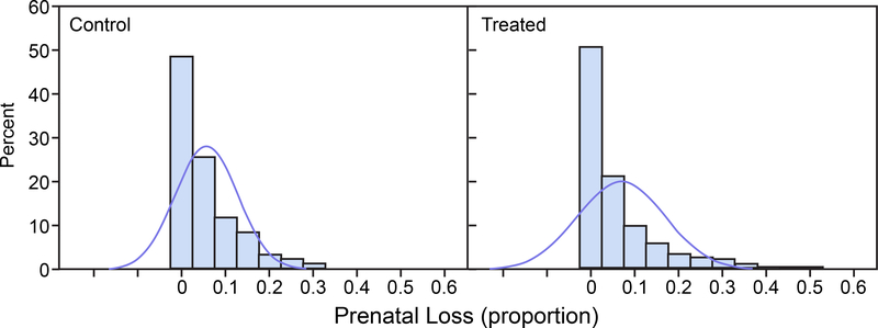
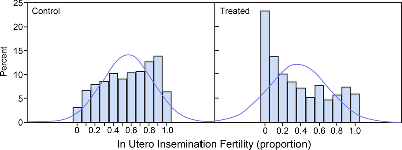
For each of the untransformed control group and treated group distributions, 1,000 random variates were drawn from a beta distribution with parameters corresponding to the original data means and standard deviations presented in Table 1 and are displayed in Figure 1 for prenatal loss and in Figure 2 for IUI fertility. Normal distribution density functions having the same sample means and sample standard deviations as the beta densities are superimposed in the histograms. Figure 1 shows that the prenatal loss distributions are skewed toward the 0 boundary for both the control and treated groups. Figure 2 shows that for IUI fertility the control group beta distribution is nearly uniformly distributed across the entire range of proportions 0 to 1 and the treated group beta distribution is skewed toward the 0 boundary. For both prenatal loss and IUI fertility appreciable portions of the approximating normal distributions, which are the basis for the power calculations, extend below the parameter space boundary at 0 and/or above the boundary at 1. The histograms were generated with SAS (Release 9.3, SAS Institute Inc.), PROC UNIVARIATE.

FIGURE 1.

Prenatal Loss. Histograms of 1,000 simulated beta-distributed random variates with means and standard deviations (SD) as in the control group (left panel) and treated group (right panel). Normal distribution density functions with the same mean and SD are superimposed on the histograms.

FIGURE 2.

In Utero Insemination Fertility. Histograms of 1,000 simulated beta-distributed random variates with means and standard deviations (SD) as in the control group (left panel) and treated group (right panel). Normal distribution density functions with the same mean and SD are superimposed on the histograms.

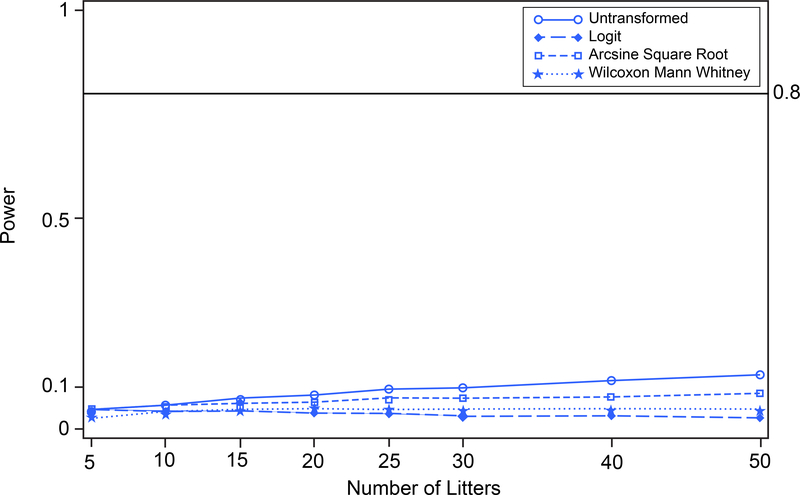
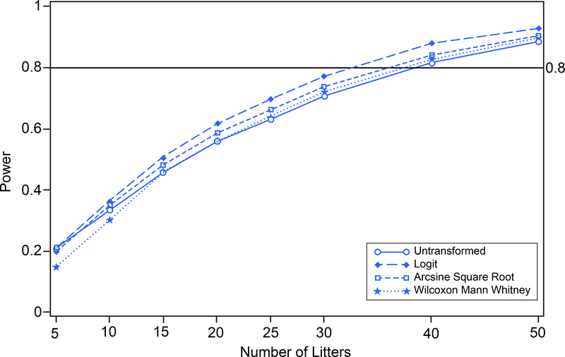
To compare how the different approaches perform when the data are skewed toward the zero boundary, we conducted additional analyses with the above datasets for prenatal loss and IUI, but with the mean proportions shifted to produce illustrative scenarios; standard deviations were unaffected (see Table 1). With the group mean proportions as originally presented in the data, for prenatal loss none of the procedures have sufficient power to be able to detect differences between the two treatment groups, or therefore distinguish among one another (Figure 8). For IUI fertility, the group mean proportions as given in the data were relatively far from the boundary of the parameter space and the power associated with each of the procedures was about the same (Figure 12). The shifts in assumed response proportion means were chosen to illustrate and clarify the methodological points made in the text. Namely, if the means were moved closer to the boundaries there was greater separation among the power curves corresponding to the different transformations. If the means were moved away from the boundaries there was less difference among the power curves for the various methods. For prenatal loss, two such scenarios were evaluated. In the first scenario, the control group was shifted toward zero and the treated group was unchanged. In the second scenario, the control group remained at original values while the treated group was shifted farther from the zero boundary. For IUI, one scenario was evaluated where both the control and treated groups were simultaneously shifted toward the zero boundary while maintaining the distance between the response proportions of the two groups.

FIGURE 8.

Prenatal Loss. Power versus number of litters for untransformed, logit-transformed, and arcsine square root-transformed proportions and Wilcoxon Mann Whitney procedure on 10,000 simulated random variates.

FIGURE 12.

In Utero Insemination Fertility. Power versus number of litters for untransformed, logit-transformed, and arcsine square root-transformed proportions and Wilcoxon Mann Whitney procedure on 10,000 simulated random variates.

RESULTS

The group population means and standard deviations of the individual litter proportions are displayed in Table 1 for the two binary endpoints – prenatal loss and IUI fertility, based on the results reported in Narotsky et al. (2013).

For IUI fertility, the mean proportions are about 1.2 to 1.9 standard deviations from 0. In contrast, for prenatal loss the mean proportions are much closer to the lower boundary of 0: the control mean proportion is about 0.75 standard deviations from the lower bound of 0 and the treated group mean proportion is just 0.69 standard deviations from 0.

Arcsine Square Root Transformation

For the arcsine square root transformation (Snedecor & Cochran, 1967), the natural parameter space is (0, π/2) ≈ (0, 1.57). Transformed values must be within this range to back transform to physically meaningful values. If ≡ observed mean litter proportion (p) with standard deviation σ among litters, then the asymptotic standard deviation of arcsine (√) is σ/(2√[p(1-p)]) (Warton & Hui, 2011). Note that the arcsine square root transformation is not a variance stabilizing transformation for the two endpoints above because of the extra binomial variation resulting from the litter-to-litter variation within groups.

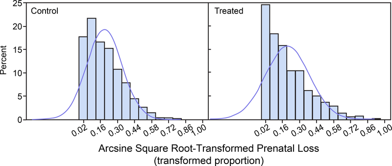
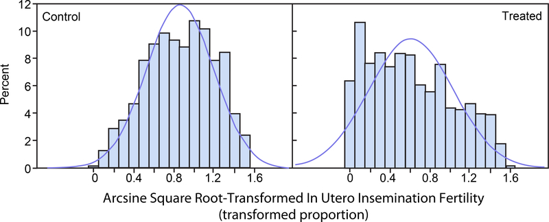
Figures 3 and 4 display histograms of the arcsine square root transformations of the beta distributed random variates displayed in Figures 1 and 2. Figure 3 corresponds to prenatal loss and Figure 4 corresponds to IUI fertility. The histograms of the arcsine square root-transformed proportions are less skewed than those of the untransformed proportions. Nonetheless, the approximating normal distributions have appreciable portions below the zero boundary for both the control and treated groups for prenatal loss (Figure 3) and for the treated group for IUI (Figure 4). These portions of the distribution outside the transformed domain do not correspond to physically meaningful transformed proportions.

FIGURE 3.

Arcsine Square Root-Transformed Prenatal Loss. Histograms of 1,000 simulated arcsine square root transforms of beta-distributed random variates with means and standard deviations (SD) as in the control group (left panel) and treated group (right panel). Normal distribution density functions with the same mean and SD are superimposed on the histograms.

FIGURE 4.

Arcsine Square Root-Transformed In Utero Insemination Fertility. Histograms of 1,000 simulated arcsine square root transforms of beta-distributed random variates with means and standard deviations (SD) as in the control group (left panel) and treated group (right panel). Normal distribution density functions with the same mean and SD are superimposed on the histograms.

Logit Transformation

For the logit transformation the issue of the closeness of the parameter to the zero boundary does not arise because the support of the logit transformation parameter space runs from minus infinity to infinity. There is no boundary to the parameter space. Thus, asymptotic normal distribution theory on which the inferences on the transformations are based is more nearly applicable with typical sample sizes.

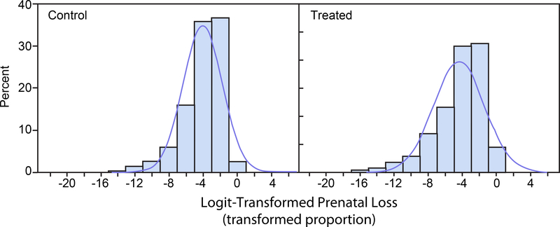
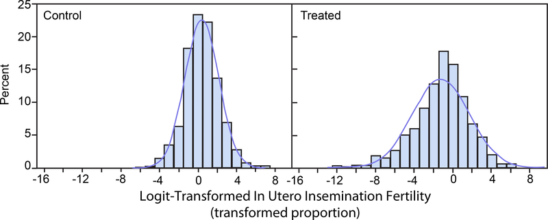
Figures 5 and 6 display histograms of the logit transformations of the beta distributed random variates displayed in Figures 1 and 2. Figure 5 corresponds to prenatal loss and Figure 6 corresponds to IUI fertility. The histograms of the logit-transformed proportions are more nearly symmetric than the histograms of the untransformed proportions and of the arcsine square root-transformed proportions. The approximating normal distributions lie entirely within the transformed logit domain (−∞, ∞).

FIGURE 5.

Logit-Transformed Prenatal Loss. Histograms of 1,000 simulated logit transforms of beta distributed random variates with means and standard deviations as in the control group (left panel) and the treated group (right panel). Normal distribution density functions with the same means and standard deviations are superimposed on the histograms.

FIGURE 6.

Logit-Transformed In Utero Insemination Fertility. Histograms of 1,000 simulated logit transforms of beta distributed random variates with means and standard deviations as in the control group (left panel) and the treated group (right panel). Normal distribution density functions with the same means and standard deviations are superimposed on the histograms.

Test Size and Power Analyses for Prenatal Loss

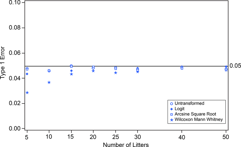
Type 1 error and power were estimated by simulation for prenatal loss based on two-sample one-tailed t-tests for untransformed, logit-transformed, and arcsine square root-transformed proportions, as well as the Wilcoxon Mann Whitney procedure on the ranked, untransformed data. Simulation was performed using SAS (Release 9.3); simulation code is provided in the supplemental material. The simulated untransformed proportions were generated based on beta distributed random variates with population means and standard deviations shown in Table 1. Estimated type 1 error and power were based on 10,000 simulations with assumed numbers of litters per group equal to 5, 10, 15, 20, 25, 30, 40, and 50. Figure 7 shows that tests based on untransformed proportions, logit-transformed proportions, arcsine square root-transformed proportions, and the Wilcoxon Mann Whitney procedure each maintain type 1 error 0.05 under the null hypothesis. Figure 8 shows that there is virtually no power to detect differences between the control group and the treated group (see Table 1) with the untransformed, the logit-transformed, the arcsine square root-transformed proportions, or the Wilcoxon Mann Whitney procedure, even with 50 litters per group.

FIGURE 7.

Prenatal Loss. Type 1 error versus number of litters for untransformed, logit-transformed, and arcsine square root-transformed proportions and Wilcoxon Mann Whitney procedure on 10,000 simulated random variates.

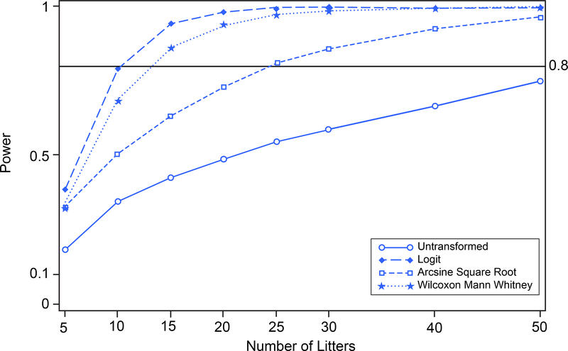
To make comparisons of the power attained with no transformation, arcsine square root transformation, logit transformation, and rank transformation under different situations, the prenatal loss data set was shifted in two different data scenarios (Table 1). For each different data scenario, type 1 error simulations were carried out and the results were as in Figure 7; each transformation maintained its type 1 error 0.05 under the null hypothesis. In the first scenario, the control group was shifted toward zero (to 0.0273) and the treated group was unchanged. A power analysis corresponding to a two-sample one-tailed t-test with type 1 error 0.05 and 5 to 50 litters per group was carried out by simulation with 10,000 simulations. The results of the power analysis with the shifted control group are shown in Figure 9. Tests based on the logit-transformed proportions have greater power than those based on untransformed proportions, on arcsine square root-transformed proportions, or on the Wilcoxon Mann Whitney test. Power of 80% can be attained with approximately 10 litters per group based on the logit transform, with approximately 25 litters per group based on the arcsine square root transform, with fewer than 15 litters per groups based on the Wilcoxon Mann Whitney test, and cannot be attained with even 50 litters per group based on the untransformed proportions. This relatively favorable performance of the logit transform-based approach becomes increasingly pronounced when the distributions of the data are skewed toward the boundary of the parameter space.

FIGURE 9.

Prenatal Loss (control group shifted toward zero). Power versus number of litters for untransformed, logit-transformed, and arcsine square root-transformed proportions and Wilcoxon Mann Whitney procedure on 10,000 simulated random variates. Control group population mean proportion is changed to 0.0273.

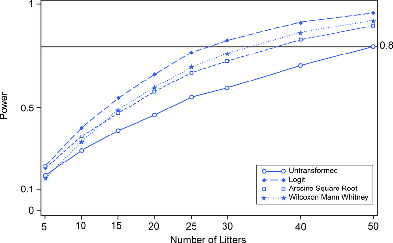
In the second alternative data scenario, the treated group was shifted farther from the zero boundary to separate the mean proportions in the control and treated groups. The treated group response proportion was 0.100 while the control group response proportion remained at 0.057. The standard deviations in the control and treated groups remained as in the original data set (see Table 1). This moved the treated group response rate farther away from the boundary of the parameter space. The results of the simulated power vs. number of litters per group based on one-tailed tests are shown in Figure 10. Again, the logit transformation results in greater power than the Wilcoxon Man Whitney test, the arcsine square root transformation, or no transformation. Note that the power resulting from the arcsine square root transformation is closer to that resulting from the logit transformation or the Wilcoxon Man Whitney test than in Figure 9 because the distributions of the observed proportions are less skewed, consequently the distributions of the transformed proportions are more nearly contained within the physically meaningful portion of the parameter space.

FIGURE 10.

Prenatal Loss (treated group shifted away from zero). Power versus number of litters for untransformed, logit-transformed, and arcsine square root-transformed proportions and Wilcoxon Mann Whitney procedure on 10,000 simulated random variates. Treated group population mean proportion is changed to 0.1000.

Test Size and Power Analyses for In Utero Insemination Fertility

The results in this section, for the endpoint IUI fertility, parallel those in the previous section. Type 1 error and power were estimated by simulation based on two-sample one-tailed t-tests for untransformed, logit-transformed, and arcsine square root-transformed proportions, and the Wilcoxon Mann Whitney procedure. The simulated untransformed proportions were generated based on beta distributed random variates with mean and variance shown in Table 1. Estimated type 1 error and power were based on 10,000 simulations with assumed numbers of litters per group equal to 5, 10, 15, 20, 25, 30, 40, and 50. Figure 11 shows that tests based on untransformed proportions, logit-transformed proportions, arcsine square root-transformed proportions, and the Wilcoxon Mann Whitney procedure each maintained type 1 error 0.05 under the null hypothesis. Figure 12 shows that the test based on the logit-transformed proportions had greater power than the tests based on the other procedures, but all four procedures had nearly the same power. This is because the mean response proportions in both the control and treated groups are both within the range of 0.3 to 0.7; the near linearity in this range (away from the boundaries of the parameter space) results in little difference among the transformations (Holland, 2017).

FIGURE 11.

In Utero Insemination Fertility. Type 1 error versus number of litters for untransformed, logit-transformed, and arcsine square root-transformed proportions and Wilcoxon Mann Whitney procedure on 10,000 simulated random variates.

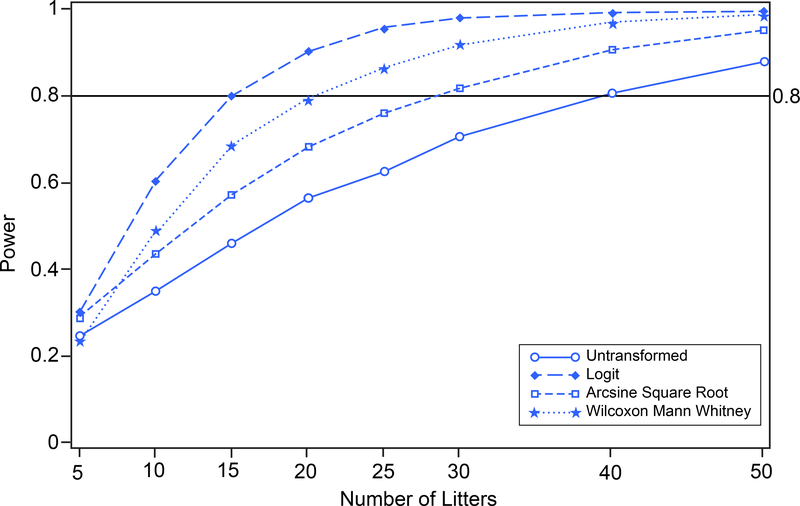
To separate the power curves, and thereby show the different strengths of the different approaches, the assumed mean fertility response proportions were moved closer to the boundary of the parameter space while maintaining the difference between the two group mean fertility response proportions. The control group mean response proportion was assumed to be 0.408 and the treated group mean response proportion was assumed to be 0.229 while the standard deviations for both groups remained the same as in the original dataset (see Table 1). The results of the power analysis are shown in Figure 13. Tests based on logit-transformed proportions had greater power than all the other approaches evaluated, followed by the Wilcoxon Mann Whitney analysis which outperformed the arcsine square root analysis. The analysis based on untransformed proportions had the least power of the four approaches.

FIGURE 13.

In Utero Insemination Fertility (control and treated groups shifted toward zero). Power versus number of litters for untransformed, logit-transformed, and arcsine square root-transformed proportions and Wilcoxon Mann Whitney procedure on 10,000 simulated random variates. Control group population mean proportion is changed to 0.408; treated group population mean proportion is changed to 0.229.

DISCUSSION

When making statistical inferences about binary responses and proportions, normalizing transformations of the proportions are often first carried out and inferences are made in the transformed domain. The aim is to improve approximations to asymptotic normal distributional results in the transformed domain with small to moderate sample sizes and thereby improve the accuracy of inferences based on asymptotic normal theory. In the mid 1900’s the arcsine square root transformation was suggested for analyses in toxicology and the environmental sciences (Chen, 2006) because it is a normalizing and variance stabilizing transformation for binomially distributed proportional data that exclude 0 and 1. However, proportions are not always binomially distributed. They may be more variable than would be predicted by the binomial distribution. This would be the case if there are litter effects (i.e., litter-to-litter variation in the control or treatment groups). This frequently occurs with litter data in developmental toxicology studies. Proportional data with variation exceeding binomial variation can also arise from non-binary data, such as the ratio of two continuous variables, e.g., organ weight to body weight ratio (Warton & Hui, 2011). In such situations the arcsine square root transformation may no longer be variance stabilizing.

The theory underlying the normalizing transformations assumes that the means of the distributions of the proportions or their transforms are multiple standard deviation units from the boundaries of the parameter spaces and their approximate large sample normal distributions are nearly completely interior to the parameter space [0, 1] or its transform (Snedecor & Cochran, 1967; Bromily & Thacker, 2002). Operationally, this means that the observed proportions are multiple standard deviations from the boundary values 0 and 1. In such situations, the arcsine square root is known to be an approximate normalizing transformation because the approximating normal distribution can extend multiple standard deviations in each direction. The approximating normal distribution after an arcsine square root transformation is assumed to lie nearly entirely within the bounds of the region. However, when the means of the observed proportions are close in standard deviation units to the boundary values of 0 or 1, the distribution of the arcsine square root-transformed proportions can be very skewed and may not be well approximated by a normal distribution. The approximating normal distribution often has a sizable portion of its probability mass outside the bounds of the parameter region. The distributions of untransformed litter proportions are then skewed toward the boundary. This is illustrated for the group distributions of the proportions for prenatal loss (Figure 1) and IUI fertility (Figure 2). The distributions of differences of group means of untransformed litter proportions will have relatively high probability mass at or near 0. The normalizing transformations reduce the extent of skewness toward the boundary of the distributions of transformed litter proportions. The distributions of differences of group means of transformed litter proportions will have relatively less probability mass at or near 0 and will therefore have greater probability content in the tails. This is true to some extent with the arcsine square root transformation and to a greater extent with the logit transformation. Thus, the arcsine square root transformation results in greater power than the untransformed proportions, and the logit transformation results in greater power than the arcsine square root transformation.

The arcsine square root transformation may not be preferred as a normalizing transformation for analysis when the distributions of the observed proportions are skewed to the boundary values of 0 or 1, such as is illustrated in Figure 3 and the treated group in Figure 4. In such cases the logistic transformation and logistic regression may be preferable to the arcsine square root transformation. Chen (2006) suggests the use of the logistic normalizing transformation (alternatively referred to as the “logit” transformation) and logistic regression to fit predictive models to litter-based proportions.

Warton & Hui (2011) compared the logit transformation with the arcsine square root transformation for the analysis of proportions. They argue that the logit transformation is a preferable alternative for multiple reasons. The logit-transformed space is infinite whereas the arcsine square root transformation space is bounded (0 to π/2 (≈1.57)). This implies that values in the logit-transformed space do not reach or cross the boundaries of the parameter space whereas values in the arcsine square root-transformed space may cross parameter boundaries. With the arcsine square root transformation in regression situations where extrapolation below 0 or above 1.57 may occur, a monotonic relation in the arcsine square root space can lead to nonmonotonic predictions in the back-transformed space of proportions (Warton & Hui, 2011). As a simple illustrative example of the arcsine back transformation not preserving monotonicity, if arcsine(√p(x)) = 1+x, a monotonically increasing relation in the arcsine square root-transformed space, then p(−2)=0.71, p(−0.25) =0.46, p(0.25)=0.90, p(1)=0.83. The relation in the back-transformed space of proportions is no longer monotonic, and so can lead to results that are not physically meaningful. This non-monotonicity in the back-transformed space is impossible with the logit transformation because the logit transformation space is unbounded.

An additional advantage of the logit transformation is the regression slope in the logit transformation space has a physically interpretable meaning whereas that in the arcsine square root transformation space does not. Namely if p(x) varies as a linear function of a predictor variable x, e.g., logit(p(x)) = α+βx, then the slope β has the physical interpretation that a unit increase in x (i.e., from x to x+1) corresponds to a multiple factor change e^β in the odds ratio p(x)/(1-p(x)) (Warton & Hui, 2011).

With the arcsine square root transformation, if the means of the observed response proportions are close to the boundaries 0 or 1, normal distribution approximations to the distributions of the transformed proportions will extend beyond the parameter space boundaries 0 or 1.57. Thus, portions of their distributions will correspond to values with physically uninterpretable back-transformed values. This is seen in Figures 3 and 4. However, with logit transformation, the transformed parameter space is infinite, and such boundary issues do not occur so that the entire distributions have physically meaningful back-transformed values. This is seen in Figures 5 and 6. This results in greater sensitivity and power for inferences based on logit-transformed proportions compared to inferences based on arcsine square root-transformed proportions. A similar consideration applies to sensitivity and power for inferences based on logit-transformed proportions compared to inferences based on untransformed proportions. The improved performance of the logit becomes more apparent the more the response proportions are skewed toward the 0 or 1 boundaries. This is illustrated in Figure 9 for prenatal loss and in Figure 13 for IUI fertility.

An alternative approach to the analysis of litter-based proportions that commonly appears in the developmental toxicology literature is the use of nonparametric test procedures such as the Wilcoxon Mann Whitney rank-based test for two group comparisons (e.g. treated vs. control) or its extension to the Kruskal-Wallis test for overall comparisons among multiple groups. Such tests do not have issues associated with parameter space boundaries that are present with procedures based on untransformed proportions or arcsine square root transformed proportions. The rank transformation retains information only about the ordering of responses but loses information about their relative differences. In the power analysis examples in this paper, when the means of the response parameters are close to the boundaries of the parameter space, the power of the Wilcoxon Mann Whitney procedure exceeds the power of tests based on untransformed or arcsine square root-transformed proportions but is less than the power of tests based on logit transformed proportions.

Although the NTP has previously used arcsine square root transformation for analysis of litter-based proportional data (e.g., NTP, 2004), more recent studies have used mixed effects logistic regression analysis for the analysis of the individual animal data (i.e., 0’s and 1’s) (e.g., NTP, 2012; Catlin et al., 2018). The treatment group means and standard deviations are modeled as fixed effects and the replicate litter effects within treatment groups are modeled as random effects, with litter response rates varying randomly within treatment groups. Their models also include covariates that adjust for variation because of secondary variates that can be observed but not controlled. This approach can be used for power analysis at the planning stage as well as for post-experiment data analysis. It can be implemented in the SAS PROC NLMIXED procedure (Li, Lingsma, Steyerberg, & Sesaffre, 2011), or in many stand-alone programs.

When analyzing data, if an observed sample litter proportion is equal to 0 or 1, the logit transform is undefined. A small continuity correction ε is often incorporated into the logit transformation (Trikalinos, Trow, & Schmid, 2013), where ε, a small positive quantity, is added to proportions of 0 and subtracted from proportions of 1. After adjustment, for p’s close to 0, logit(p) ≡ log[(p+ε)/(1-p-ε)]. For p’s close to 1, logit(p) ≡ log[(p-ε)/(1-p+ε)]. For example, if ε=0.0001, then 0 values are adjusted to 0.0001 and values of 1 are adjusted to 0.9999. The adjusted logit transformation is called an “empirical” logit transformation. Such continuity corrections are used when logit transformations are first carried out on the raw proportion data and then inference procedures such as t-tests, analysis of variance tests, or regression analyses are carried out on the logit transformed proportions. This is a more classical approach to statistical analysis. The more modern approach using mixed effects logistic regression models fit to the individual animal binary responses by maximum likelihood analysis does not require the use of continuity corrections. The need for continuity corrections and empirical logits is not needed at the planning stage, even when utilizing the classical approach, because power analyses are usually based on the continuous large sample beta distribution approximation to the exact discrete beta binomial distribution of litter proportions. Response proportions of 0 or 1 are not realized for the beta distribution.

When the observed mean proportions are in the 0.3 to 0.7 range, the transformations have little difference among them as their curves are essentially linear in this range (Holland, 2017). However, we have demonstrated that when the observed proportions are close to zero in standard deviation units, tests based on untransformed proportions or based on the arcsine square root transformation can have less power than the logit transformation to detect departures from the control group response. In the comparisons of the analyses of our different illustrative dataset scenarios, the superiority of the logit-transformation approach becomes increasingly pronounced when the response proportions are closer to the boundaries of the parameter space. Given that many litter-based proportional data sets in developmental and reproductive toxicology are typically skewed (e.g., malformation rate, prenatal loss), the choice of statistical analysis of the data is an important consideration. The current findings support logit transformation (or logistic regression) as a preferred option, particularly when the data are skewed.

The authors suggest that henceforth “LOL” in toxicologists’ texts stand for “LOVE OF LOGIT”!

REFERENCES

- Agresti A (2012). Chapter 6. Building, checking, and applying logistic regression models, 6.6 Sample size and power considerations. In: Categorical Data Analysis, 3rd Ed. New York: Wiley. pp. 237–240. [Google Scholar]
- Bromiley PA & Thacker NA (2002). The effects of an arcsin square root transformation on a binomial distributes quantity. Tina Memo 2002–007. Medical School, University of Manchester, www.tina-vision.net/docs/memos_statistics.php [Google Scholar]
- Casella G & Berger RL (2002). Statistical Inference (Vol. 2). Pacific Grove, CA: Duxbury. pp. 337–442. [Google Scholar]
- Catlin N, Waidyanatha S, Mylchreest E, Miller-Pinsler L, Cunny H, Foster P, Sutherland V, & McIntyre B (2018). Embryo-fetal development studies with the dietary supplement vinpocetine in the rat and rabbit. Birth Defects Research Part B Developmental and Reproductive Toxicology, 110(10), 883–896 [DOI] [PMC free article] [PubMed] [Google Scholar]
- Chen JJ (2006). Statistical analysis for developmental and reproductive toxicologists. In: Hood RD, editor. Developmental and Reproductive Toxicology: A Practical Approach, 2nd ed. Boca Raton, FL: CRC Press. p 697–711. [Google Scholar]
- Efron B (1986). Discussion: Jackknife, bootstrap and other resampling methods in regression analysis. Annals of Statistics, 14(4), 1301–1304. [Google Scholar]
- Feller W (1966). The Central Limit Theorem. In: An Introduction to Probability Theory and Its Applications, Volume II. Chapter VIII, Section 4. New York: Wiley & Sons, Inc. pp. 258–265 [Google Scholar]
- Glass GV, Peckham PD, & Sanders JR (1972). Consequences of failure to meet assumptions underlying the fixed effects analyses of variance and covariance. Review of Educational Research, 42(3), 237–288. [Google Scholar]
- Holland S (2017). Transformations of proportions and percentages. Data Analysis in the Geosciences. University of Georgia, http://strata.uga.edu/8370/rtips/proportions.html [Google Scholar]
- Jaeger TF (2008). Categorical data analysis: away from ANOVAs (transformation or not) and towards logit mixed models. Journal of Memory and Language, 59, 434–446. [DOI] [PMC free article] [PubMed] [Google Scholar]
- Klinefelter GR (2002). Actions of toxicants on the structure and function of the epididymis. In: Robaire B and Hinton BT, editors. The epididymis – from molecules to clinical practice. New York: Kluwer Academic/Plenum Publisher. p 353–369. [Google Scholar]
- Li B, Lingsma HF, Steyerberg EW, & Lesaffre E (2011). Logistic random effects regression models: A comparison of statistical packages for binary and ordinal outcomes. BMC Medical Research Methodology, 11, 77. [DOI] [PMC free article] [PubMed] [Google Scholar]
- Narotsky MG, Klinefelter GR, Goldman JM, Best DS, McDonald A, Strader LF, Suarez JD, Murr AS, Thillainadarajah I, Hunter ES 3rd, Richardson SD, Speth TF, Miltner RJ, Pressman JG, Teuschler LK, Rice GE, Moser VC, Luebke RW, & Simmons JE (2013). Comprehensive assessment of a chlorinated drinking water concentrate in a rat multigenerational reproductive toxicity study. Environ Sci Technol 47, 10653–10659. [DOI] [PubMed] [Google Scholar]
- National Institute of Standards Technology (NIST)/SEMATECH. (2012). e-Handbook of Statistical Methods 1.3.6.6.17. Beta Distribution. https://www.itl.nist.gov/div898/handbook/eda/section3/eda366h.htm
- National Toxicology Program (NTP). (2004). Final Study Report. Developmental toxicity evaluation for benzophenone (CAS No. 119–61-9) administered by gavage to New Zealand White rabbits on gestational days 6 through 29. NTP Study No. TER-99–001. [Google Scholar]
- National Toxicology Program (NTP). (2012). NTP Technical Report on the Toxicology and Carcinogenesis Study of Styrene-Acrylonitrile Trimer in F344/N Rats (Perinatal and Postnatal Feed Studies). NTP TR 573. NIH Publication No. 12–5915. [PubMed] [Google Scholar]
- Snedecor GW & Cochran WG (1967). Statistical Methods. 6th Edition. Ames IA, The Iowa State University [Google Scholar]
- Trikalinos TA, Trow P, & Schmid CH (2013). Simulation-Based Comparison of Methods for MetaAnalysis of Proportions and Rates. Rockville, MD, US Department of Health and Human Services. [PubMed] [Google Scholar]
- Warton DI & Hui FK (2011). The arcsine is asinine: the analysis of proportions in ecology. Ecology, 92, 3–10. [DOI] [PubMed] [Google Scholar]
- Williams DA (1975). The analysis of binary responses from toxicological experiments involving reproduction and teratogenicity. Biometrics, 31, 949. [PubMed] [Google Scholar]
Associated Data
This section collects any data citations, data availability statements, or supplementary materials included in this article.