Modelling personal cautiousness during the COVID-19 pandemic: a case study for Turkey and Italy

Abstract

Although policy makers recommend or impose various standard measures, such as social distancing, movement restrictions, wearing face masks and washing hands, against the spread of the SARS-CoV-2 pandemic, individuals follow these measures with varying degrees of meticulousness, as the perceptions regarding the impending danger and the efficacy of the measures are not uniform within a population. In this paper, a compartmental mathematical model is presented that takes into account the importance of personal cautiousness (as evidenced, for example, by personal hygiene habits and carefully following the rules) during the COVID-19 pandemic. Two countries, Turkey and Italy, are studied in detail, as they share certain social commonalities by their Mediterranean cultural codes. A mathematical analysis of the model is performed to find the equilibria and their local stability, focusing on the transmission parameters and investigating the sensitivity with respect to the parameters. Focusing on the (assumed) viral exposure rate, possible scenarios for the spread of COVID-19 are examined by varying the viral exposure of incautious people to the environment. The presented results emphasize and quantify the importance of personal cautiousness in the spread of the disease.

Introduction

Mathematical modelling of the transmission of infectious diseases has a history of about a hundred years in mathematical epidemiology [18]. The so-called SIR models have been widely studied for understanding the spread of many infectious diseases and have become an important tool for controlling outbreaks and determining treatment and vaccination policies [1, 4, 13, 21, 34]. The current pandemic, coronavirus disease 2019 (COVID-19), has attracted the interest of researchers from different scientific areas and once again highlighted the importance of appropriate mathematical modelling in developing control strategies.

COVID-19 is caused by a novel coronavirus identified as Severe Acute Respiratory Syndrome Coronavirus 2 (SARS-CoV-2) by the World Health Organization (WHO) on January 12, 2020 [36]. Coronaviruses (CoVs) are enveloped positive-sense zoonotic RNA respiratory viruses that cause a variety of diseases in mammals and birds [11]. The native form of CoVs is rarely transmitted among humans but their mutant forms are capable of human-to-human transmission [25]. There have been two outbreaks of the of CoVs in the last two decades: the Severe Acute Respiratory Syndrome Coronavirus (SARS-CoV, China, 2002) and the Middle Eastern Respiratory Syndrome Coronavirus (MERS-CoV, Saudi Arabia, 2012). The studies point out that, despite main differences in their structure and epidemiology, both SARS-CoV and MERS-CoV are airborne viruses, and there is also strong evidence of possible airborne transmission of SARS-CoV-2 [25, 39, 40]. Virus transmission is thought to occur by direct (coughing, sneezing, speaking etc.) or indirect (contaminated surfaces etc.) contact through droplets and aerosols [24].

By July 12, 2020, the number of confirmed COVID-19 cases was 12,552,765, with 561,617 deaths, according to the Word Health Organization [37]. The fatality rate of COVID-19 is estimated to be lower than SARS and MERS but the potential transmissibility seems to be higher [26]. At the time of writing of this paper there was still no vaccine available against coronaviruses for use in humans [41]. Therefore, governments have implemented several measures, such as social distancing rules, movement restrictions, and wearing face masks, against the spread of the disease during the 2020 SARS-CoV-2 pandemic. On the other hand, such measures have been followed by individuals with varying degrees of meticulousness, as the perceptions regarding the impending danger and the efficacy of the measures differed widely within a population.

The Ministry of Health of the Republic of Turkey declared the first case of COVID-19 on March 10, 2020. Partial travel restrictions were imposed on February 23, 2020, and people who entered Turkey were isolated for 14 days. On March 16, 2020, restrictions were tightened: schools and universities switched to distance education and people with chronic diseases or disabilities and seniors over 60 were given administrative leave [8]. The Ministry of Health decided to implement a partial quarantine to control the spread of the disease and maintain a balance of social and economic factors. Lock-down rules were imposed on senior people of age 65 and above on March 21, 2020, and on those under the age of 20 on April 3, 2020. According to the official demography report of Turkish Statistical Institute (TUIK), these two groups constitute approximately 33% of the total population of Turkey (83,154,997) [33]. In fact, the proportion in lock-down might actually be higher since the government has recommended self-isolation for all citizens and supported partially working from home. At that point, the self-discipline of citizens, i.e. being cautious or incautious, had a role on the spread of the disease.

As of June 2020, Italy had the third highest number of COVID-19 cases in the world after the USA and Spain, the fourth highest prevalence of the disease after Spain, Belgium, and the USA, and the third highest total number of deaths attributed to COVID-19 after the USA and the UK in the ongoing pandemic [5]. The first case of COVID-19 in Italy was reported on January 23, 2020. The Italian government introduced travel restrictions on January 30, and people who have come into close contact with confirmed cases were directed to a mandatory quarantine for 14 days. All public events and educational activities were suspended in five regions of Italy starting February 23. Starting March 8, all movement of citizens, except those necessary for work, health, or food, were restricted. The ban was extended to all non-indispensable activities on March 23, 2020 [20, 30].

Since the emergence of the current pandemic, many researchers have studied various mathematical and computational models to understand the dynamics of COVID-19 as it spreads locally and globally [28], in an effort to provide recommendations to policy makers to predict the behaviour of the disease and eventually to bring it under control [2, 3, 12, 16, 17, 19]. In this paper, a mathematical model is developed for describing the transmission dynamics of COVID-19 in Turkey by taking the cautiousness of people into account. In this context, cautiousness refers to diligently following the rules regarding self-isolation and social distance. The results of this study are compared to the data of Italy, as both countries share some common elements of Mediterranean culture (close social distances, crowded social life, collective eating-drinking habits, and so on) that might have influenced the transmission rate of the disease.

The paper is organized as follows. In Sect. 2, the standard SIR model is modified to distinguish cautious and incautious individuals. In Sect. 3, the basic reproduction number ${\mathcal{R}}_0$ is calculated and the local stability of equilibria is studied. In Sect. 4.1, the sensitivity of the basic reproduction number ${\mathcal{R}}_0$ with respect to the model parameters is discussed. In Sect. 4.2, transmission parameters are estimated and numerical simulations are performed according to data from Turkey and Italy. The paper concludes in Section  5 with a discussion of the results.

Compartmental model with cautious individuals

In this section, a mathematical model is developed based on the standard compartmental modelling approach of Kermack and McKendrick [18]. Here, the focus is on the effect of cautiousness on the human-to-human disease transmission during the pandemic. Cautiousness involves many fuzzy parameters like obeying isolation rules, wearing face masks, paying attention to social distances, etc. It is not easy to find data to measure the efficient probability of being cautious. However, different scenarios could be studied for estimating such social aspects of the disease dynamics.

In this model, the population is assumed to be distributed homogeneously and divided into four compartments: $S_C$: cautious susceptible individuals, $S_I$: incautious susceptible individuals, $I_C$: cautious infected individuals, and $I_I$: incautious infected individuals. At this time there is no scientific consensus on whether infected individuals gain immunity after recovery. WHO has reported that there is not enough scientific evidence for the existence of antibody-mediated immunity; on the other hand, recent studies point to the possible role of T cells in the long-term protection from reinfection with SARS-CoV-2. The present paper concentrates on the transmission mechanism of the disease, and in particular on the spreading phase of the infection rather than treatment and reinfection. A separate compartment for recovered/removed individuals is not considered due to insufficient medical and biological knowledge about SARS-CoV-2 [6, 38]. It is assumed that the population has a constant size $N=N_C+N_I=S_C+S_I+I_C+I_I$. The relation between the compartments $S_C$ and $S_I$ is ignored, based on the assumption that cautious individuals try to minimize contact with incautious people. An additional compartment, E, is included that represents the concentration of SARS-CoV-2 viruses in the environment that are ready for attaching and transferring their genetic material to humans. It is assumed that the virulence function has a bounded Hill type form $f(E)=\frac{E}{K+E}$ with a constant carrying capacity K. With the above assumptions, the system of Eq. (1) is obtained for describing the transmission dynamics of the disease:

$$\begin{array}{c}\hfill \left\{\begin{array}{c}{\displaystyle \frac{\mathrm{d}{S}_C}{\mathrm{d}t}}=pbN-{\displaystyle \frac{{\beta }_C{S}_C{I}_C}{N_C}}-{\displaystyle \frac{{\beta }_{\mathit{IC}}{S}_C{I}_I}{N_I}}\hfill \\ -{\beta }_{\mathit{CE}}{S}_C\left({\displaystyle \frac{E}{K+E}}\right)-\mu S_C\hfill \\ {\displaystyle \frac{\mathrm{d}{I}_C}{\mathrm{d}t}}={\displaystyle \frac{{\beta }_C{S}_C{I}_C}{N_C}}+{\displaystyle \frac{{\beta }_{\mathit{IC}}{S}_C{I}_I}{N_I}}\hfill \\ +{\beta }_{\mathit{CE}}{S}_C\left({\displaystyle \frac{E}{K+E}}\right)-(\mu +d)I_C\hfill \\ {\displaystyle \frac{\mathrm{d}{S}_I}{\mathrm{d}t}}=qbN-{\displaystyle \frac{{\beta }_I{S}_I{I}_I}{N_I}}-{\displaystyle \frac{{\beta }_{\mathit{CI}}{S}_I{I}_C}{N_C}}\hfill \\ -{\beta }_{\mathit{IE}}r{S}_I\left({\displaystyle \frac{E}{K+E}}\right)-\mu S_I\hfill \\ {\displaystyle \frac{\mathrm{d}{I}_I}{\mathrm{d}t}}={\displaystyle \frac{{\beta }_I{S}_I{I}_I}{N_I}}+{\displaystyle \frac{{\beta }_{\mathit{CI}}{S}_I{I}_C}{N_C}}\hfill \\ +{\beta }_{\mathit{IE}}r{S}_I\left({\displaystyle \frac{E}{K+E}}\right)-(\mu +d)I_I\hfill \\ {\displaystyle \frac{\mathrm{d}E}{\mathrm{d}t}}=k_1{I}_C+k_2{I}_I-wE\hfill \end{array}\right)\end{array}$$ 1

A schematic flowchart describing the model (1) is given in Fig. 1 and the parameters of the model are described in Table 1.

Fig. 1.

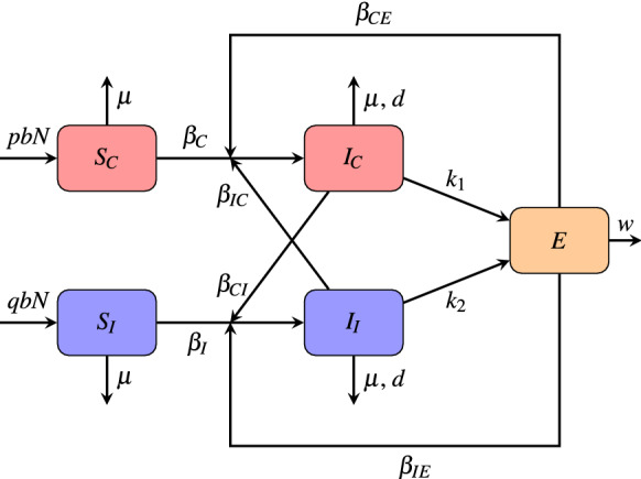
Flowchart of the model (1)

Table 1.

Parameters of the model (1)

Parameters	Description
b	Natural birth rate
p	Probability of being cautious
$q=1-p$	Probability of being incautious
${\beta }_C$	Transmission rate among cautious people
${\beta }_I$	Transmission rate among incautious people
${\beta }_{\mathit{CE}}$	Transmission rate from environment to cautious people
${\beta }_{\mathit{IE}}$	Transmission rate from environment to incautious people
${\beta }_{\mathit{IC}}$	Transmission rate from incautious to cautious people
${\beta }_{\mathit{CI}}$	Transmission rate from cautious to incautious people
r	A comparison factor for viral exposure
$\mu$	Natural death rate
d	Disease-related death rate and recovery rate
$k_1$	Virus exposure rate by cautious people
$k_2$	Virus exposure rate by incautious people
w	Decay rate of viruses
K	Assumed carrying capacity of the virus reservoir

Stability analysis of the model

Local stability of equilibria

The compartments of infection in model (1) are represented by the symbols $I_C,I_I$, and E. The disease-free equilibrium (DFE) of the model is found by setting the derivatives to zero and substituting $I_C=I_I=0$. Since there are no infected individuals at the beginning, it is assumed that there are no viruses in the environment at all, i.e. $E=0$. Thus, the disease-free equilibrium has the form $E_{\mathit{df}}=(S_C^{\ast },0,S_I^{\ast },0,0)$, where $S_C^{\ast }={\displaystyle \frac{\mathit{pbN}}{\mu }}$ and $S_I^{\ast }={\displaystyle \frac{\mathit{qbN}}{\mu }}$.

The endemic equilibrium corresponds to the infectious case and has the form $E_d=(S_C^{\ast },I_C^{\ast },S_I^{\ast },I_I^{\ast },E^{\ast })$, where $S_C^{\ast }$, $S_I^{\ast }$, and $E^{\ast }$ are given by

$$\begin{array}{cc}\hfill S_C^{\ast }& ={\displaystyle \frac{pbN-(\mu +d)I_C^{\ast }}{\mu }}\hfill \\ \hfill S_I^{\ast }& ={\displaystyle \frac{qbN-(\mu +d)I_I^{\ast }}{\mu }}\hfill \\ \hfill E^{\ast }& ={\displaystyle \frac{k_1{I}_C^{\ast }+k_2{I}_I^{\ast }}{w}},\hfill \end{array}$$ 2

and $I_C^{\ast }$ and $I_I^{\ast }$ are the solutions of the equations

$$\begin{array}{cc}& A_1{I}_C^3+B_1{I}_C^2+C_1{I}_C+D_1{I}_C^2{I}_I\hfill \\ \hfill & +E_1{I}_C{I}_I+F_1{I}_C{I}_I^2+G_1{I}_I^2+H_1{I}_I=0\hfill \\ \hfill & A_2{I}_I^3+B_2{I}_I^2+C_2{I}_I+D_2{I}_I^2{I}_C\hfill \\ \hfill & +E_2{I}_I{I}_C+F_2{I}_I{I}_C^2+G_2{I}_C^2+H_2{I}_C=0.\hfill \end{array}$$

An algebraic calculation of the associated constants yields

$$\begin{array}{cc}\hfill A_1& =(\mu +d)k_1{\beta }_C{N}_I,\hfill \\ \hfill B_1& =(\mu +d)N_I(\mu k_1{N}_C+Kw{\beta }_C+K{k}_1{N}_C{\beta }_{\mathit{CE}})\hfill \\ \hfill & -Nbp{k}_1{\beta }_C{N}_I,\hfill \\ \hfill C_1& =\mu (\mu +d)Kw{N}_C{N}_I-NbpK(w{\beta }_C{N}_I+k_1{\beta }_{\mathit{CE}}{N}_C{N}_I),\hfill \\ \hfill D_1& =(\mu +d)(k_2{\beta }_C{N}_I+k_1{\beta }_{\mathit{IC}}{N}_C),\hfill \\ \hfill E_1& =(\mu +d)N_C(\mu k_2{N}_I+Kw{\beta }_{\mathit{IC}}+K{k}_2{N}_I{\beta }_{\mathit{CE}})\hfill \\ \hfill & -Nbp(k_1{\beta }_{\mathit{IC}}{N}_C+k_2{\beta }_C{N}_I),\hfill \\ \hfill F_1& =(\mu +d)k_2{\beta }_{\mathit{IC}}{N}_C,\hfill \\ \hfill G_1& =-Nbp{k}_2{N}_C{\beta }_{\mathit{IC}},\hfill \\ \hfill H_1& =-NbpK{N}_C(w{\beta }_{\mathit{IC}}+k_2{N}_I{\beta }_{\mathit{CE}}),\hfill \\ \hfill A_2& =(\mu +d)k_1{\beta }_C{N}_I,\hfill \\ \hfill B_2& =(\mu +d)N_C(\mu k_2{N}_I+Kw{\beta }_I+rK{k}_2{N}_I{\beta }_{\mathit{IE}})\hfill \\ \hfill & -Nbp{k}_1{\beta }_C{N}_I,\hfill \\ \hfill C_2& =\mu (\mu +d)Kw{N}_C{N}_I-NbqK(w{\beta }_I{N}_C+r{k}_2{\beta }_{\mathit{IE}}{N}_C{N}_I),\hfill \\ \hfill D_2& =(\mu +d)(k_1{\beta }_I{N}_C+k_2{\beta }_{\mathit{CI}}{N}_I),\hfill \\ \hfill E_2& =(\mu +d)N_I(\mu k_1{N}_C+Kw{\beta }_{\mathit{CI}}+rK{k}_1{N}_C{\beta }_{\mathit{IE}})\hfill \\ \hfill & -Nbp(k_2{\beta }_{\mathit{CI}}{N}_I+k_1{\beta }_I{N}_C),\hfill \\ \hfill F_2& =(\mu +d)k_1{\beta }_{\mathit{CI}}{N}_I,\hfill \\ \hfill G_2& =-Nbq{k}_1{N}_I{\beta }_{\mathit{CI}},\hfill \\ \hfill H_2& =-NbqK{N}_I(w{\beta }_{\mathit{CI}}+k_1{N}_C{\beta }_{\mathit{IE}}).\hfill \end{array}$$

The Jacobian matrix J of the system (1) is given by

$$\begin{array}{c}\hfill J=\left[\begin{array}{ccccc}-{\overline{A}}_1-\mu & -{\overline{B}}_1& 0& -{\overline{C}}_1& -{\overline{D}}_1\\ {\overline{A}}_1& {\overline{B}}_1-(\mu +d)& 0& {\overline{C}}_1& {\overline{D}}_1\\ 0& -{\overline{C}}_2& -{\overline{A}}_2-\mu & -{\overline{B}}_2& -{\overline{D}}_2\\ 0& {\overline{C}}_2& {\overline{A}}_2& {\overline{B}}_2-(\mu +d)& {\overline{D}}_2\\ 0& k_1& 0& k_2& -w\end{array}\right]\end{array}$$

where ${\overline{A}}_1={\beta }_C{\displaystyle \frac{I_C}{N_C}}+{\beta }_{\mathit{IC}}{\displaystyle \frac{I_I}{N_I}}+{\beta }_{\mathit{CE}}{\displaystyle \frac{E}{K+E}}$, ${\overline{B}}_1={\beta }_C{\displaystyle \frac{S_C}{N_C}}$, ${\overline{C}}_1={\beta }_{\mathit{IC}}{\displaystyle \frac{S_C}{N_I}}$, ${\overline{D}}_1={\beta }_{\mathit{CE}}{S}_C{\displaystyle \frac{K}{{(K+E)}^2}}$, ${\overline{A}}_2={\beta }_I{\displaystyle \frac{I_I}{N_I}}+{\beta }_{\mathit{CI}}{\displaystyle \frac{I_C}{N_C}}+{\beta }_{\mathit{IE}}{\displaystyle \frac{\mathit{rE}}{K+E}}$, ${\overline{B}}_2={\beta }_I{\displaystyle \frac{S_I}{N_I}}$, ${\overline{C}}_2={\beta }_{\mathit{CI}}{\displaystyle \frac{S_I}{N_C}}$, ${\overline{D}}_2={\beta }_{\mathit{IE}}{S}_I{\displaystyle \frac{\mathit{rK}}{{(K+E)}^2}}$.

Linearisation of the system (1) around the disease-free equilibrium $E_{\mathit{df}}=\left({\displaystyle \frac{\mathit{pbN}}{\mu }},,,0,,,{\displaystyle \frac{\mathit{qbN}}{\mu }},,,0,,,0\right)$ yields the Jacobian matrix

$$\begin{array}{c}\hfill J_{\mathit{df}}=\left[\begin{array}{ccccc}-\mu & -{\beta }_C{\displaystyle \frac{b}{\mu }}& 0& -{\beta }_{\mathit{IC}}{\displaystyle \frac{\mathit{pbN}}{\mu N_I}}& -{\beta }_{\mathit{CE}}{\displaystyle \frac{\mathit{pbN}}{\mu K}}\\ 0& {\beta }_C{\displaystyle \frac{b}{\mu }}-(\mu +d)& 0& {\beta }_{\mathit{IC}}{\displaystyle \frac{\mathit{pbN}}{\mu N_I}}& {\beta }_{\mathit{CE}}{\displaystyle \frac{\mathit{pbN}}{\mu K}}\\ 0& -{\beta }_{\mathit{CI}}{\displaystyle \frac{\mathit{qbN}}{\mu N_C}}& -\mu & -{\beta }_I{\displaystyle \frac{b}{\mu }}& -{\beta }_{\mathit{IE}}{\displaystyle \frac{\mathit{qbN}}{\mu K}}\\ 0& {\beta }_{\mathit{CI}}{\displaystyle \frac{\mathit{qbN}}{\mu N_C}}& 0& {\beta }_I{\displaystyle \frac{b}{\mu }}-(\mu +d)& {\beta }_{\mathit{IE}}{\displaystyle \frac{\mathit{qbN}}{\mu K}}\\ 0& k_1& 0& k_2& -w\end{array}\right].\end{array}$$

Two eigenvalues of $J_{\mathit{df}}$ are ${\lambda }_{1,2}=-\mu$, which are negative by biological assumptions. The other eigenvalues of $J_{\mathit{df}}$ are calculated through the submatrix $J_1$

$$\begin{array}{cc}\hfill J_1=& \left[\begin{array}{ccc}{\beta }_C{\displaystyle \frac{b}{\mu }}-(\mu +d)& {\beta }_{\mathit{IC}}{\displaystyle \frac{\mathit{pbN}}{\mu N_I}}& {\beta }_{\mathit{CE}}{\displaystyle \frac{\mathit{pbN}}{\mu K}}\\ {\beta }_{\mathit{CI}}{\displaystyle \frac{\mathit{qbN}}{\mu N_C}}& {\beta }_I{\displaystyle \frac{b}{\mu }}-(\mu +d)& {\beta }_{\mathit{IE}}{\displaystyle \frac{\mathit{qbN}}{\mu K}}\\ k_1& k_2& -w\end{array}\right]\hfill \\ \hfill =& \left[\begin{array}{ccc}{a}_1& b_1& c_1\\ a_2& b_2& c_2\\ k_1& k_2& -w\end{array}\right].\hfill \end{array}$$

The characteristic polynomial of $J_1$ has the form

$$\begin{array}{c}\hfill {\lambda }^3+A{\lambda }^2+B\lambda +C,\end{array}$$ 3

where

$$\begin{array}{cc}\hfill A& =w-a_1-b_2,\hfill \\ \hfill B& =a_1{b}_2-w(a_1+b_2)-b_1{a}_2-c_1{k}_1-c_2{k}_2,\hfill \\ \hfill D& =w(a_1{b}_2-b_1{a}_2)+(c_1{k}_1+c_2{k}_2)(a_1+b_2)\hfill \\ \hfill & -k_1(a_1{c}_1+b_1{c}_2)-k_2(a_2{c}_1+b_2{c}_2).\hfill \end{array}$$ 4

By the Routh–Hurwitz stability criterion, all roots of the characteristic polynomial have negative real parts if and only if $A>0$ and $AB>C>0$. These inequalities constitute the condition for the local asymptotic stability of the disease-free equilibrium.

The Jacobian matrix $J_d$ of the system (1) at the endemic equilibrium $E_d$ is

$$\begin{array}{c}\hfill J_d=\left[\begin{array}{ccccc}-a_1-\mu & -b_1& 0& -c_1& -d_1\\ a_1& b_1-\mu -d& 0& c_1& d_1\\ 0& -c_2& -a_2-\mu & -b_2& -d_2\\ 0& c_2& a_2& b_2-\mu -d& d_2\\ 0& k_1& 0& k_2& -w\end{array}\right],\end{array}$$

where $a_1={\beta }_C{\displaystyle \frac{I_C}{N_C}}+{\beta }_{\mathit{IC}}{\displaystyle \frac{I_I}{N_I}}+{\beta }_{\mathit{CE}}{\displaystyle \frac{E}{K+E}}$, $b_1={\beta }_C{\displaystyle \frac{S_C}{N_C}}$, $c_1={\beta }_{\mathit{IC}}{\displaystyle \frac{S_C}{N_I}}$, $d_1={\beta }_{\mathit{CE}}{S}_C{\displaystyle \frac{K}{{(K+E)}^2}}$, $a_2={\beta }_I{\displaystyle \frac{I_I}{N_I}}+{\beta }_{\mathit{CI}}{\displaystyle \frac{I_C}{N_C}}+{\beta }_{\mathit{IE}}{\displaystyle \frac{\mathit{rE}}{K+E}}$, $b_2={\beta }_I{\displaystyle \frac{S_I}{N_I}}$, $c_2={\beta }_{\mathit{CI}}{\displaystyle \frac{S_I}{N_C}}$, $d_2={\beta }_{\mathit{IE}}{S}_I{\displaystyle \frac{\mathit{rK}}{{(K+E)}^2}}$.

The corresponding characteristic polynomial has the form

$$\begin{array}{c}\hfill {\lambda }^5+A{\lambda }^4+B{\lambda }^3+C{\lambda }^2+D\lambda +F,\end{array}$$ 5

where the coefficients can be calculated explicitly (see “Appendix A”). By the Routh–Hurwitz stability criterion, all roots of the characteristic polynomial (5) have negative real parts if and only if $ABC>C^2+A^{2}D$ and $(AD-F)(ABC-C^2-A^{2}D)>F{(AB-C)}^2+A{F}^2$. These inequalities constitute the condition for the local asymptotic stability of the endemic equilibrium.

Basic reproduction rate ${\mathcal{R}}_0$

The average number of secondary infections generated by an infectious individual in a completely susceptible population is called the basic reproduction number ${\mathcal{R}}_0$. In the following, ${\mathcal{R}}_0$ is calculated using the method of next generation matrix [9, 34]. The matrix of new infections F and matrix of the remaining transition terms V are given by

$$\begin{array}{c}\hfill F=\left[\begin{array}{ccc}{\beta }_C{\displaystyle \frac{b}{\mu }}& {\beta }_{\mathit{IC}}{\displaystyle \frac{\mathit{pbN}}{\mu N_I}}& {\beta }_{\mathit{CE}}{\displaystyle \frac{b}{\mu K}}\\ {\beta }_{\mathit{CI}}{\displaystyle \frac{\mathit{qbN}}{\mu N_C}}& {\beta }_I{\displaystyle \frac{b}{\mu }}& {\beta }_{\mathit{IE}}{\displaystyle \frac{b}{\mu K}}\\ 0& 0& 0\end{array}\right]\end{array}$$ 6

and

$$\begin{array}{c}\hfill V=\left[\begin{array}{ccc}\mu +d& 0& 0\\ 0& \mu +d& 0\\ -k_1& -k_2& w\end{array}\right],\end{array}$$ 7

respectively. The basic reproduction number is then obtained from the spectral radius of the matrix

$$\begin{array}{c}\hfill F{V}^{-1}=\left[\begin{array}{ccc}{a}_1+k_1{b}_1& c_1+k_2{b}_1& (\mu +d)b_1\\ c_2+k_1{b}_2& a_2+k_2{b}_2& (\mu +d)b_2\\ 0& 0& 0\end{array}\right]\end{array}$$ 8

where $a_1={\displaystyle \frac{b{\beta }_C}{\mu (\mu +d)}}$, $a_2={\displaystyle \frac{b{\beta }_I}{\mu (\mu +d)}}$, $b_1={\displaystyle \frac{b{\beta }_{\mathit{CE}}}{\mu (\mu +d)wK}}$, $b_2={\displaystyle \frac{b{\beta }_{\mathit{IE}}}{\mu (\mu +d)wK}}$, $c_1={\displaystyle \frac{pbN{\beta }_{\mathit{IC}}}{\mu (\mu +d)N_I}}$, $c_2={\displaystyle \frac{qbN{\beta }_{\mathit{CI}}}{\mu (\mu +d)N_C}}$. Hence, the basic reproduction number is calculated as

$$\begin{array}{c}\hfill {\mathcal{R}}_0=\left\{\begin{array}{cc}{\displaystyle \frac{a_1+a_2+b_1{k}_1+b_2{k}_2}{2}},& \text{if}\Delta \le 0\\ {\displaystyle \frac{a_1+a_2+b_1{k}_1+b_2{k}_2+\sqrt{\Delta }}{2}},& \text{if}\Delta >0\end{array}\right)\end{array}$$ 9

where $\Delta =a_1^2+a_2^2+b_1^2{k}_1^2+b_2^2{k}_2^2+2a_2{b}_2{k}_2-2a_2{a}_1-2a_2{k}_1{b}_1-2a_1{b}_2{k}_2+2b_1{k}_1{b}_2{k}_2+2a_1{b}_1{k}_1+4c_1{c}_2+4c_2{k}_2{b}_1+4c_1{k}_1{b}_2$.

The disease-free equilibrium is locally asymptotically stable if ${\mathcal{R}}_0<1$ and unstable if ${\mathcal{R}}_0>1$ according to the theorem given in [34].

Parameter estimation and simulations

The model (1) is now fitted to the data of confirmed COVID-19 cases in Turkey and Italy [37]. Since the main interest will be the estimation of transmission parameters, some of the disease-specific parameters are given fixed values based on statistical and biological knowledge from the literature. The values and units of the parameters can be found with their associated references in Table 2 for Turkey and in Table 3 for Italy.

Table 2.

Parameters of the model (1) for Turkey

Parameters	Value	Units	Source
b	$3.512\times {10}^{-5}$	day${}^{-1}$	Assumed based on [33]
p	0.4	dim.less	Assumed based on quarantine policy
$q=1-p$	0.6	dim.less	Assumed based on quarantine policy
d	0.0627	day${}^{-1}$	[29]
$\mu$	$3.512\times {10}^{-5}$	day${}^{-1}$	[33]
${\beta }_C$	0.00114	day${}^{-1}$	Estimated
${\beta }_{\mathit{CE}}$	0.000056	day${}^{-1}$	Estimated
${\beta }_I$	0.00985	day${}^{-1}$	Estimated
${\beta }_{\mathit{IE}}$	0.000098	day${}^{-1}$	Estimated
${\beta }_{\mathit{IC}}$	0.00711	day${}^{-1}$	Estimated
$k_1$	1	day${}^{-1}$	Assumed
$k_2$	3	day${}^{-1}$	Assumed
w	5	day${}^{-1}$	Assumed (after [27, 32])
K	19,000	copies/day	Assumed (after [10])

Table 3.

Parameters of the model (1) for Italy

Parameters	Value	Units	Source
b	$3.3\times {10}^{-5}$	day${}^{-1}$	Assumed based on [15]
p	0.6	dim.less	Assumed based on quarantine policy
$q=1-p$	0.4	dim.less	Assumed based on quarantine policy
d	0.085	day${}^{-1}$	[29]
$\mu$	$3.3\times {10}^{-5}$	day${}^{-1}$	[15]
${\beta }_C$	0.0079	day${}^{-1}$	Estimated
${\beta }_{\mathit{CE}}$	0.000037	day${}^{-1}$	Estimated
${\beta }_I$	0.049	day${}^{-1}$	Estimated
${\beta }_{\mathit{IE}}$	0.00018	day${}^{-1}$	estimated
${\beta }_{\mathit{IC}}$	0.009	day${}^{-1}$	Estimated
$k_1$	1	day${}^{-1}$	Assumed
$k_2$	3	day${}^{-1}$	Assumed
w	5	day${}^{-1}$	Assumed (after [27, 32])
K	19,000	copies/day	Assumed (after [10])

Turkish Statistical Institute (TUIK) has reported the life expectancy in Turkey to be around 78 in year 2018 and the total population is around 83 million in 2020 [33]. Therefore, the natural death rate is taken to be 1/78 per year. By the assumption that the total population does not change significantly in a few months, it follows that $b=\mu =(1/78)/365$ per day, i.e., the natural birth rate and the natural death rate are equal. It is assumed that 40% of the total population of Turkey is cautious, based on the quarantine policies consisting of a curfew effective for 33% of the total population, and recommendations of self-isolation and working from home.

The life expectancy in Italy was reported to be around 83 years in 2018 by the Italian National Institute of Statistics [15]. Thus, $b=\mu =(1/83)/365$ per day, i.e., the natural birth rate and the natural death rate are chosen equal for a period of short time. The total population is around 60 million in 2020 [15]. Since Italy set up strict lock-down rules, the percentage of the cautious people is set at 60% [31].

Viruses belonging to the family Coronaviridae can survive on inanimate surfaces between three hours and three days [32, 35]. Therefore, the decay rate of virus is assumed to be between 1/8–3 days and a random value from this interval is taken. The duration of viral shedding is between 6–37 days from initial viral detection [23]. Furthermore, it is reported that the asymptomatic transmission of the COVID-19 is an important point in understanding the transmission mechanism of the disease, and the transmissibility of the asymptomatic cases among close contacts is comparable to the symptomatic cases [14]. In clinical samples the median concentrations of R- and N-gene RNA for CoVs are detected between $5.2\times {10}^2$ and $1.2\times {10}^6$ copies/ml during 4 days of virus replication [10]. In view of these biological considerations, cautiousness may have a high impact on minimizing the viral shedding rate. Consequently, it is initially assumed that the virus exposure rate of an incautious individual is three times higher than a cautious one, i.e. $k_1=1/\text{day}$ and $k_2=3/\text{day}$, respectively.

Intuitively, the interaction between the cautious susceptible individuals and the incautious infected individuals should be very low. Therefore, the transmission rate from cautious one to incautious ones is taken to be zero for all simulations; i.e., ${\beta }_{\mathit{CI}}=0$. There are five remaining model parameters, ${\beta }_C$, ${\beta }_{\mathit{CE}}$, ${\beta }_I$, ${\beta }_{\mathit{IE}}$, ${\beta }_{\mathit{IC}}$, that need to be estimated from real data. The model 1 is fitted to the total number of confirmed infected cases for Turkey for the period March 13–July 12, and for Italy for the period February 24–July 12, 2020. The vector of the parameters $q=({\beta }_C$, ${\beta }_{\mathit{CE}}$, ${\beta }_I$, ${\beta }_{\mathit{IE}}$, ${\beta }_{\mathit{IC}})$ of the model (1) is evaluated by solving a nonlinear least squares problem with positive constraints according to the data set $u(t)=I_I(t)+I_C(t)$ [7]. An objective function $J(\theta )$ is defined as the sum of the squares of the errors

$$\begin{array}{c}\hfill J(\theta )=\sum {(y_i-f(x_i,\theta ))}^2\end{array}$$ 10

where $y_i$ is the points of the data set and $f(x_i,\theta )$ is the model function with the vector of unknown parameters $\theta$. To minimize the objective function $J(\theta )$, the nonlinear least square minimization routine ‘lsqnoline’ of MATLAB is used. The model (1) is numerically solved using the ODE solver ‘ode45’ [22]. The parameter values used in the simulations are given in Tables 2 and 3.

Sensitivity analysis

A sensitivity analysis is carried out to determine the robustness of the model to the parameter values that are correlated with the basic reproduction number ${\mathcal{R}}_0$. The sensitivity indices are calculated to determine the parameters that are most efficient by the transmission of COVID-19 in Turkey and Italy. Following the sensitivity approach given in [21], a normalized sensitivity index of a variable ${\mathcal{R}}_0$ with respect to the parameter p is defined as

$$\begin{array}{c}\hfill {ϵ}_{{\mathcal{R}}_0}^p={\displaystyle \frac{\partial {\mathcal{R}}_0}{\partial p}}\times {\displaystyle \frac{p}{{\mathcal{R}}_0}}.\end{array}$$ 11

The values of the sensitivity indices for the parameter in Tables 2 and 3 are presented in Table 4, which shows the significance of ${\beta }_{\mathit{IE}}$, $k_2$, and w. For both countries, it can be concluded that an increase of the value of ${\beta }_{\mathit{IE}}$ and $k_2$ promote the basic reproduction number, whereas an increase of the value of w diminishes ${\mathcal{R}}_0$.

Table 4.

Sensitivity of the parameters effect the basic reproduction number ${\mathcal{R}}_0$

Parameters	Sensitivity index (Turkey)	Sensitivity index (Italy)
${\beta }_C$	0.0002031	0.0011269
${\beta }_I$	0.0273442	0.1380501
${\beta }_{\mathit{CE}}$	0.0558663	0.0361162
${\beta }_{\mathit{IE}}$	0.9123331	0.8137572
${\beta }_{\mathit{IC}}$	0.0042530	0.0109494
$k_1$	0.0601194	0.0470657
$k_2$	0.9080801	0.8028077
w	-0.9681995	-0.8498734

Simulations

The numerical solution of the model (1) is plotted with estimated parameters in Fig. 2 together with the data set of Turkey, which explains quite well the spread-dynamics of COVID-19 in the first 120 days. Since the model fits the given data set according to the presented scenario, the possible number of cautious and incautious infectious people in Turkey over a period of 200 days is simulated as shown in Fig. 3. It can be seen from Fig. 2 that the actual number of cases increases while the model curve starts to flatten more and less after the 100th day of pandemic. This point correlates well with the date June 1, 2020, on which Turkey officially announced relaxing most isolation measures, which explains the increasing behaviour of the data.

Fig. 2.

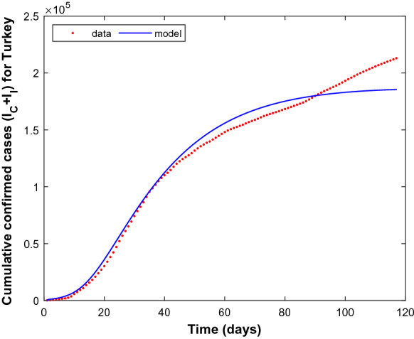
Cumulative confirmed cases for Turkey for the period March 13, 2020 to July 12, 2020. Dashed line (red) denotes the reported cumulative cases and solid line (blue) denotes the simulation result. (Color figure online)

Fig. 3.

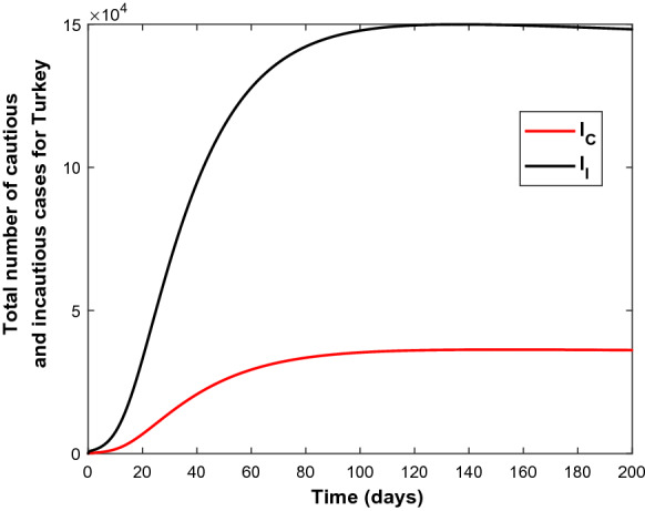
The variation of the infected classes $I_C$ (bottom) and $I_I$ (top) using the parameters from Table 2

Similarly, Fig. 4 indicates the success of parameter estimation using the real data set of Italy. Figure 5 shows the estimates for the number of cautious and incautious people in Italy over 200 days from the beginning of the pandemic.

Fig. 4.

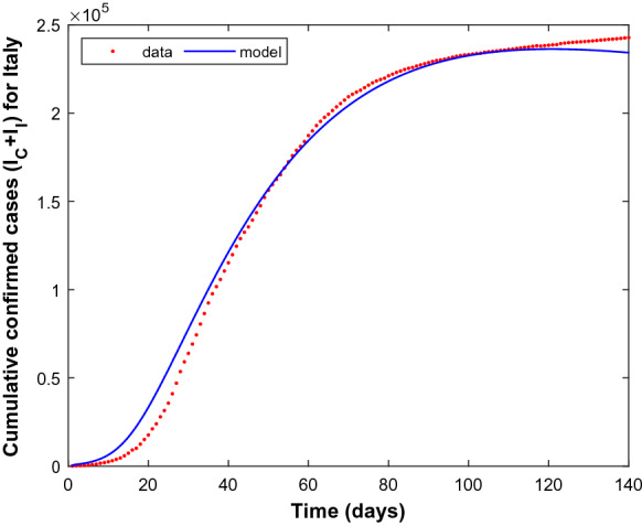
Cumulative confirmed cases for Italy for the period February 24, 2020–July 12, 2020. Dashed line (red) denote the reported cumulative cases and solid line (blue) denotes the simulation result. (Color figure online)

Fig. 5.

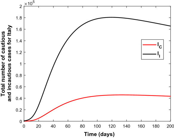
The variation of the infected classes $I_C$ (bottom) and $I_I$ (top) using the parameters from Table 3

Since high sensitivity of the parameters ${\beta }_{\mathit{IE}}$ and $k_2$ is observed, these two parameters are manipulated to observe the change of number of infectious people both in Turkey and in Italy. The results are shown in Figs. 6, 7, 8, and 9.

Fig. 6.

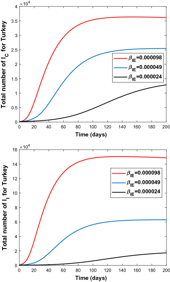
Graphs of $I_C(t)$ and $I_I(t)$ for various values of the transmission rate ${\beta }_{\mathit{IE}}=$ 0:000098 (top), ${\beta }_{\mathit{IE}}=$ 0:000049 (middle), ${\beta }_{\mathit{IE}}=$ 0:000024 (bottom) for Turkey

Fig. 7.

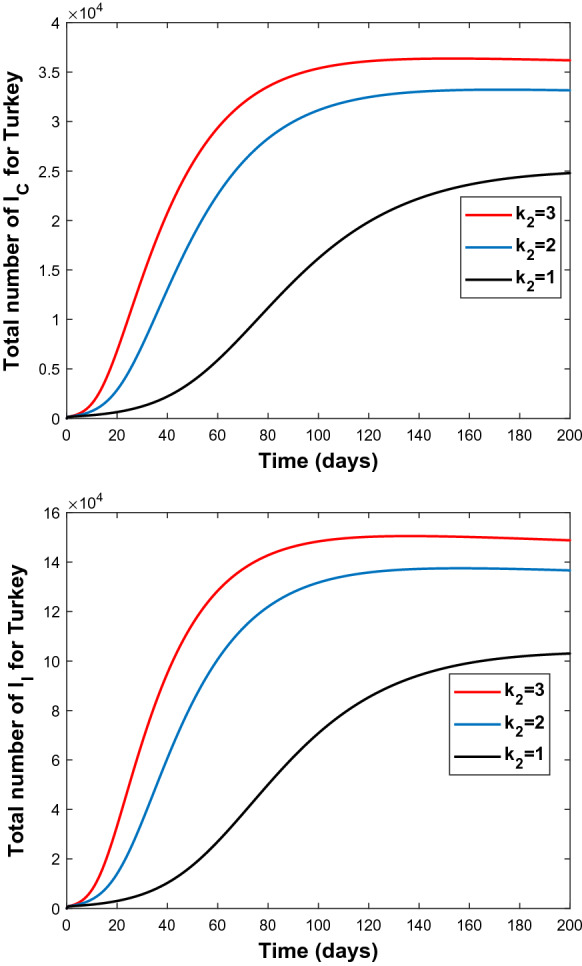
Graphs of $I_C(t)$ and $I_I(t)$ for different values of virus exposure rate by incautious people; $k_2=$ 1 (bottom), $k_2=$ 2 (middle), $k_2=$ 3 (top) for Turkey

Fig. 8.

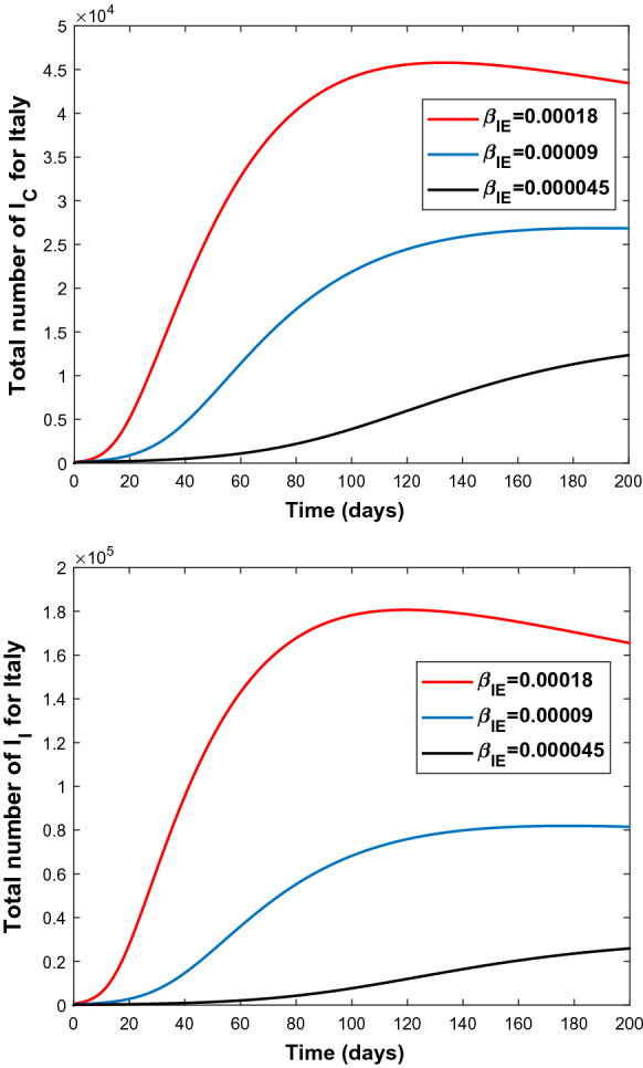
Graphs of $I_C(t)$ and $I_I(t)$ for various values of the transmission rate ${\beta }_{\mathit{IE}}=0.00018$ (top), ${\beta }_{\mathit{IE}}=0.00009$ (middle), ${\beta }_{\mathit{IE}}=0.000045$ (bottom) for Italy

Fig. 9.

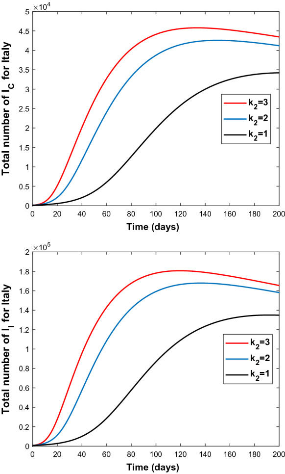
Graphs of $I_C(t)$ and $I_I(t)$ for different values of virus exposure rate by incautious people; $k_2=1$ (bottom), $k_2=2$ (middle), $k_2=3$ (top) for Italy

Finally, Fig. 10 shows the correlation between two sensitive parameters ${\beta }_{\mathit{IE}}$ and $k_2$ for both countries. While Fig. 11 indicates a linear increase of ${\mathcal{R}}_0$ with respect to ${\beta }_{\mathit{IE}}$, the value of ${\mathcal{R}}_0$ remains much higher for Turkey than for Italy.

Fig. 10.

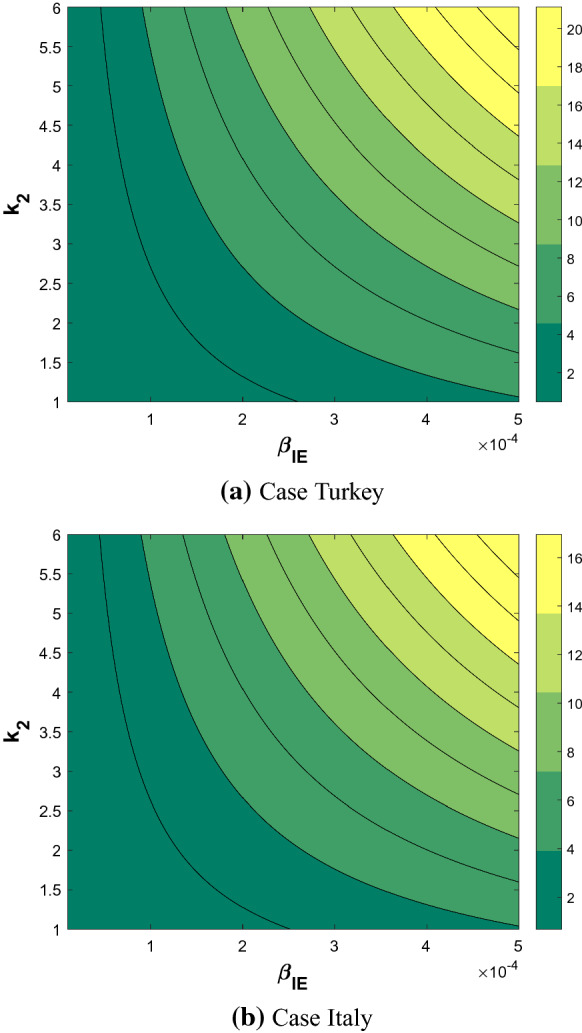
Correlation between two sensitive parameters ${\beta }_{\mathit{IE}}$ and $k_2$ for the basic reproduction rate

Fig. 11.

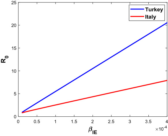
Basic reproduction number versus ${\beta }_{\mathit{IE}}$ in both countries (Turkey(top) and Italy(bottom))

Conclusions

This paper has proposed a deterministic compartmental model to understand the effect of cautiousness on the transmission of COVID-19 in Turkey and Italy, two countries that have a similar collective life typical of the Mediterranean region, which involves eating together, flexible social distance habits, crowded social places, and tight relationship of families. The local asymptotic stability of the disease-free and endemic equilibria have been determined, and the corresponding basic reproduction number ${\mathcal{R}}_0$ has been derived. Personal cautiousness is undoubtedly one of the important factors affecting the transmission rate of COVID-19 in every country. However, it is difficult to quantify cautiousness and establish the dynamics of spread under many unknown parameters. The presented results underline the sensitivity of the transmission rate representing how incautious individuals are infected from environmental sources, which implies that small changes in individuals’ habits would effect the dynamics of the pandemic strongly. The mathematical analysis supports in the current scenario that personal cautiousness may repress the pandemic in both countries. Future work may consist of the addition of a recovered compartment and a vaccination process, whose details can be added to the model as we continue to increase our knowledge of the disease, thanks to worldwide research efforts.

Appendix: the characteristic polynomial of $J_d$

The characteristic polynomial of the matrix $J_d$ is

$$\begin{array}{c}\hfill {\lambda }^5+A{\lambda }^4+B{\lambda }^3+C{\lambda }^2+D\lambda +F,\end{array}$$

where

$$\begin{array}{cc}\hfill A& =\left(2,d,+,w,+,4,\mu ,+,a_1,+,a_2,-,b_1,-,b_2\right),\hfill \\ \hfill B& =6d\mu +4w\mu +6{\mu }^2+2d{a}_1+2d{a}_2-d{b}_1-d{b}_2+w{a}_1\hfill \\ \hfill & +w{a}_2-w{b}_1-w{b}_2+3\mu a_1+3\mu a_2-3\mu b_1-3\mu b_2+a_1{a}_2\hfill \\ \hfill & -a_1{b}_2-a_2{b}_1+b_1{b}_2-c_1{c}_2-d_1{k}_1-d_2{k}_2+2dw+d^2,\hfill \\ \hfill C& =4{\mu }^3+d^{2}w+6d{\mu }^2+2d^2\mu +6w{\mu }^2+d^2{a}_1+d^2{a}_2\hfill \\ \hfill & +3{\mu }^2{a}_1+3{\mu }^2{a}_2-3{\mu }^2{b}_1-3{\mu }^2{b}_2+6dw\mu +2dw{a}_1\hfill \\ \hfill & +2dw{a}_2-dw{b}_1-dw{b}_2+4d\mu a_1+4d\mu a_2-2d\mu b_1\hfill \\ \hfill & -2d\mu b_2+3w\mu a_1+3w\mu a_2-3w\mu b_1-3w\mu b_2\hfill \\ \hfill & +2d{a}_1{a}_2-d{a}_1{b}_2-d{a}_2{b}_1-d{d}_1{k}_1-d{d}_2{k}_2+w{a}_1{a}_2\hfill \\ \hfill & -w{a}_1{b}_2-w{a}_2{b}_1+w{b}_1{b}_2-w{c}_1{c}_2+2\mu a_1{a}_2-2\mu a_1{b}_2\hfill \\ \hfill & -2\mu a_2{b}_1+2\mu b_1{b}_2-2\mu c_1{c}_2-3\mu d_1{k}_1-3\mu d_2{k}_2\hfill \\ \hfill & -a_2{d}_1{k}_1-a_1{d}_2{k}_2+b_2{d}_1{k}_1+b_1{d}_2{k}_2-c_1{d}_2{k}_1-c_2{d}_1{k}_2,\hfill \\ \hfill D& =d^2{\mu }^2+{\mu }^4+2d{\mu }^3+4w{\mu }^3+{\mu }^3{a}_1+{\mu }^3{a}_2-{\mu }^3{b}_1\hfill \\ \hfill & -{\mu }^3{b}_2+d^2{a}_1{a}_2+{\mu }^2{a}_1{a}_2-{\mu }^2{a}_1{b}_2-{\mu }^2{a}_2{b}_1+{\mu }^2{b}_1{b}_2\hfill \\ \hfill & -{\mu }^2{c}_1{c}_2-3{\mu }^2{d}_1{k}_1-3{\mu }^2{d}_2{k}_2+6dw{\mu }^2+2d^{2}w\mu \hfill \\ \hfill & +d^{2}w{a}_1+d^{2}w{a}_2+2d{\mu }^2{a}_1+d^2\mu a_1+2d{\mu }^2{a}_2+d^2\mu a_2\hfill \\ \hfill & -d{\mu }^2{b}_1-d{\mu }^2{b}_2+3w{\mu }^2{a}_1+3w{\mu }^2{a}_2-3w{\mu }^2{b}_1\hfill \\ \hfill & -3w{\mu }^2{b}_2-2\mu a_2{d}_1{k}_1-2\mu a_1{d}_2{k}_2+2\mu b_2{d}_1{k}_1\hfill \\ \hfill & +2\mu b_1{d}_2{k}_2-2\mu c_1{d}_2{k}_1-2\mu c_2{d}_1{k}_2+4dw\mu a_1\hfill \\ \hfill & +4dw\mu a_2-2dw\mu b_1-2dw\mu b_2+2dw{a}_1{a}_2-dw{a}_1{b}_2\hfill \\ \hfill & -dw{a}_2{b}_1+2d\mu a_1{a}_2-d\mu a_1{b}_2-d\mu a_2{b}_1-2d\mu d_1{k}_1\hfill \\ \hfill & -2d\mu d_2{k}_2+2w\mu a_1{a}_2-2w\mu a_1{b}_2-2w\mu a_2{b}_1\hfill \\ \hfill & +2w\mu b_1{b}_2-2w\mu c_1{c}_2-d{a}_2{d}_1{k}_1-d{a}_1{d}_2{k}_2,\hfill \\ \hfill F& =w{\mu }^4+d^{2}w{\mu }^2-{\mu }^3{d}_1{k}_1-{\mu }^3{d}_2{k}_2+2dw{\mu }^3+w{\mu }^3{a}_1\hfill \\ \hfill & +w{\mu }^3{a}_2-w{\mu }^3{b}_1-w{\mu }^3{b}_2+d^{2}w{a}_1{a}_2-d{\mu }^2{d}_1{k}_1\hfill \\ \hfill & -d{\mu }^2{d}_2{k}_2+w{\mu }^2{a}_1{a}_2-w{\mu }^2{a}_1{b}_2-w{\mu }^2{a}_2{b}_1+w{\mu }^2{b}_1{b}_2\hfill \\ \hfill & -w{\mu }^2{c}_1{c}_2-{\mu }^2{a}_2{d}_1{k}_1-{\mu }^2{a}_1{d}_2{k}_2+{\mu }^2{b}_2{d}_1{k}_1\hfill \\ \hfill & +{\mu }^2{b}_1{d}_2{k}_2-{\mu }^2{c}_1{d}_2{k}_1-{\mu }^2{c}_2{d}_1{k}_2+2dw{\mu }^2{a}_1\hfill \\ \hfill & +d^{2}w\mu a_1+2dw{\mu }^2{a}_2+d^{2}w\mu a_2-dw{\mu }^2{b}_1-dw{\mu }^2{b}_2\hfill \\ \hfill & -d\mu a_2{d}_1{k}_1-d\mu a_1{d}_2{k}_2+2dw\mu a_1{a}_2-dw\mu a_1{b}_2\hfill \\ \hfill & -dw\mu a_2{b}_1.\hfill \end{array}$$

Compliance with ethical standards

Conflict of interest

The authors declare that they have no conflict of interest.

References

- 1.Adams B, Banks H, Davidian M, Kwon HD, Tran H, Wynne S, Rosenberg E. HIV dynamics: modeling, data analysis, and optimal treatment protocols. J. Comput. Appl. Math. 2005;184(1):10–49. doi: 10.1016/j.cam.2005.02.004. [DOI] [Google Scholar]
- 2.Atangana A, Araz Sİ. Mathematical model of COVID-19 spread in turkey and south Africa: theory, methods, and applications. Adv. Differ. Equ. 2020;2020(1):1–89. doi: 10.1186/s13662-020-03095-w. [DOI] [PMC free article] [PubMed] [Google Scholar]
- 3.Barbarossa MV, Fuhrmann J, Meinke JH, Krieg S, Varma HV, Castelletti N, Lippert T. Modeling the spread of COVID-19 in Germany: early assessment and possible scenarios. PLoS ONE. 2020;15(9):e0238559. doi: 10.1371/journal.pone.0238559. [DOI] [PMC free article] [PubMed] [Google Scholar]
- 4.Castillo-Chavez C, Song B. Dynamical models of tuberculosis and their applications. Math. Biosci. Eng. 2004;1(2):361–404. doi: 10.3934/mbe.2004.1.361. [DOI] [PubMed] [Google Scholar]
- 5.Cegolon L, Pichierri J, Mastrangelo G, Cinquetti S, Sotgiu G, Bellizzi S, Pichierri G. Hypothesis to explain the severe form of COVID-19 in Northern Italy. BMJ Global Health. 2020;5(6):e002564. doi: 10.1136/bmjgh-2020-002564. [DOI] [PMC free article] [PubMed] [Google Scholar]
- 6.Chen Z, Wherry EJ. T cell responses in patients with COVID-19. Nat. Rev. Immunol. 2020;20(9):529–536. doi: 10.1038/s41577-020-0402-6. [DOI] [PMC free article] [PubMed] [Google Scholar]
- 7.Coleman TF, Li Y. An interior trust region approach for nonlinear minimization subject to bounds. SIAM J. Optim. 1996;6(2):418–445. doi: 10.1137/0806023. [DOI] [Google Scholar]
- 8.Demirbilek Y, Pehlivantürk G, Özgüler ZO, Alp Meşe E. COVID-19 outbreak control, example of Ministry of Health of Turkey. Turkish J. Med. Sci. 2020;50:489–494. doi: 10.3906/sag-2004-187. [DOI] [PMC free article] [PubMed] [Google Scholar]
- 9.Diekmann, O., Heesterbeek, J., Metz, J.: On the definition and the computation of the basic reproduction ratio R0 in models for infectious diseases in heterogeneous populations. J. Math. Biol. 28(4) (1990) [DOI] [PubMed]
- 10.Drosten C, Chiu LL, Panning M, Leong HN, Preiser W, Tam JS, Gunther S, Kramme S, Emmerich P, Ng WL, Schmitz H, Koay ESC. Evaluation of advanced reverse transcription-PCR assays and an alternative PCR target region for detection of severe acute respiratory syndrome-associated coronavirus. J. Clin. Microbiol. 2004;42(5):2043–2047. doi: 10.1128/JCM.42.5.2043-2047.2004. [DOI] [PMC free article] [PubMed] [Google Scholar]
- 11.Fehr, A.R., Perlman, S.: Coronaviruses: an overview of their replication and pathogenesis. In: Coronaviruses, pp. 1–23. Springer, New York (2015) [DOI] [PMC free article] [PubMed]
- 12.Giordano G, Blanchini F, Bruno R, Colaneri P, Filippo AD, Matteo AD, Colaneri M. Modelling the COVID-19 epidemic and implementation of population-wide interventions in Italy. Nat. Med. 2020;26(6):855–860. doi: 10.1038/s41591-020-0883-7. [DOI] [PMC free article] [PubMed] [Google Scholar]
- 13.Gölgeli M, Atay FM. Analysis of an epidemic model for transmitted diseases in a group of adults and an extension to two age classes. Hacet. J. Math. Stat. 2020;49(3):921–934. [Google Scholar]
- 14.He D, Zhao S, Lin Q, Zhuang Z, Cao P, Wang MH, Yang L. The relative transmissibility of asymptomatic COVID-19 infections among close contacts. Int. J. Infect. Dis. 2020;94:145–147. doi: 10.1016/j.ijid.2020.04.034. [DOI] [PMC free article] [PubMed] [Google Scholar]
- 15.ISTAT: Italian National Institute of Statistics. Tech. rep., Italian National Institute of Statistics (2020)
- 16.Ivorra B, Ferrández M, Vela-Pérez M, Ramos A. Mathematical modeling of the spread of the coronavirus disease 2019 (COVID-19) taking into account the undetected infections. The case of China. Commun. Nonlinear Sci. Numer. Simul. 2020;88:105303. doi: 10.1016/j.cnsns.2020.105303. [DOI] [PMC free article] [PubMed] [Google Scholar]
- 17.Jewell NP, Lewnard JA, Jewell BL. Predictive mathematical models of the COVID-19 pandemic. JAMA. 2020;323(19):1893. doi: 10.1001/jama.2020.6585. [DOI] [PubMed] [Google Scholar]
- 18.Kermack WO, McKendrick AG. A contribution to the mathematical theory of epidemics. Proc. R. Soc. Lond. Ser. A Contain. Pap. Math. Phys. Character. 1927;115(772):700–721. [Google Scholar]
- 19.Kucharski AJ, Russell TW, Diamond C, Liu Y, Edmunds J, Funk S, Eggo RM, Sun F, Jit M, Munday JD, Davies N, Gimma A, van Zandvoort K, Gibbs H, Hellewell J, Jarvis CI, Clifford S, Quilty BJ, Bosse NI, Abbott S, Klepac P, Flasche S. Early dynamics of transmission and control of COVID-19: a mathematical modelling study. Lancet. Infect. Dis. 2020;20(5):553–558. doi: 10.1016/S1473-3099(20)30144-4. [DOI] [PMC free article] [PubMed] [Google Scholar]
- 20.Lazzerini M, Putoto G. COVID-19 in Italy: momentous decisions and many uncertainties. Lancet Global Health. 2020;8(5):e641–e642. doi: 10.1016/S2214-109X(20)30110-8. [DOI] [PMC free article] [PubMed] [Google Scholar]
- 21.Martcheva M. An Introduction to Mathematical Epidemiology. Berlin: Springer-Verlag GmbH; 2015. [Google Scholar]
- 22.MATLAB-Mathworks: MATLAB version 9.4.0.813654 (R2018a). The Mathworks, Inc., Natick (2018)
- 23.Miyamae Y, Hayashi T, Yonezawa H, Fujihara J, Matsumoto Y, Ito T, Tsubota T, Ishii K. Duration of viral shedding in asymptomatic or mild cases of novel coronavirus disease 2019 (COVID-19) from a cruise ship: a single-hospital experience in Tokyo, Japan. Int. J. Infect. Dis. 2020;97:293–295. doi: 10.1016/j.ijid.2020.06.020. [DOI] [PMC free article] [PubMed] [Google Scholar]
- 24.Morawska L, Cao J. Airborne transmission of SARS-CoV-2: the world should face the reality. Environ. Int. 2020;139:105730. doi: 10.1016/j.envint.2020.105730. [DOI] [PMC free article] [PubMed] [Google Scholar]
- 25.Otter J, Donskey C, Yezli S, Douthwaite S, Goldenberg S, Weber D. Transmission of SARS and MERS coronaviruses and influenza virus in healthcare settings: the possible role of dry surface contamination. J. Hosp. Infect. 2016;92(3):235–250. doi: 10.1016/j.jhin.2015.08.027. [DOI] [PMC free article] [PubMed] [Google Scholar]
- 26.Petrosillo N, Viceconte G, Ergonul O, Ippolito G, Petersen E. COVID-19, SARS and MERS: are they closely related? Clin. Microbiol. Infect. 2020;26(6):729–734. doi: 10.1016/j.cmi.2020.03.026. [DOI] [PMC free article] [PubMed] [Google Scholar]
- 27.Quirouette C, Younis NP, Reddy MB, Beauchemin CAA. A mathematical model describing the localization and spread of influenza a virus infection within the human respiratory tract. PLoS Comput. Biol. 2020;16(4):e1007705. doi: 10.1371/journal.pcbi.1007705. [DOI] [PMC free article] [PubMed] [Google Scholar]
- 28.Rhodes, T., Lancaster, K.: Mathematical models as public troubles in COVID-19 infection control: following the numbers. Health Sociol. Rev. 1–18 (2020) [DOI] [PubMed]
- 29.Ritchie, H., Ortiz-Ospina, E., Beltekian, D., Mathieu, E., Hasell, J., Macdonald, B., Giattino, C., Roser, M., Breck Yunits, A.E.V.W., Gavrilov, D., Bergel, M., Ahmad, S., Crawford, J.: Mortality risk of COVID-19. Tech. rep., Our World In Data is a project of the Global Change Data Lab, a registered charity in England and Wales (Charity Number 1186433) (2020). https://ourworldindata.org/mortality-risk-covid
- 30.Signorelli C, Scognamiglio T, Odone A. COVID-19 in Italy: impact of containment measures and prevalence estimates of infection in the general population. Acta Bio Medica Atenei Parmensis. 2020;91(3–S):175–179. doi: 10.23750/abm.v91i3-S.9511. [DOI] [PMC free article] [PubMed] [Google Scholar]
- 31.Sjödin, H., Wilder-Smith, A., Osman, S., Farooq, Z., Rocklöv, J.: Only strict quarantine measures can curb the coronavirus disease (COVID-19) outbreak in Italy, 2020. Eurosurveillance 25(13) (2020) [DOI] [PMC free article] [PubMed]
- 32.Suman, R., Javaid, M., Haleem, A., Vaishya, R., Bahl, S., Nandan, D.: Sustainability of coronavirus on different surfaces. J. Clin. Exp. Hepatol. (2020) [DOI] [PMC free article] [PubMed]
- 33.TUIK: Adrese Dayalı Nüfus Kayıt Sistemi Sonuçları, 2019. Tech. rep., Turkish Statistical Institute (2020). http://www.tuik.gov.tr/PreHaberBultenleri.do?id=33705
- 34.van den Driessche P, Watmough J. Reproduction numbers and sub-threshold endemic equilibria for compartmental models of disease transmission. Math. Biosci. 2002;180(1–2):29–48. doi: 10.1016/S0025-5564(02)00108-6. [DOI] [PubMed] [Google Scholar]
- 35.van Doremalen N, Bushmaker T, Morris DH, Holbrook MG, Gamble A, Williamson BN, Tamin A, Harcourt JL, Thornburg NJ, Gerber SI, Lloyd-Smith JO, de Wit E, Munster VJ. Aerosol and surface stability of SARS-CoV-2 as compared with SARS-CoV-1. N. Engl. J. Med. 2020;382(16):1564–1567. doi: 10.1056/NEJMc2004973. [DOI] [PMC free article] [PubMed] [Google Scholar]
- 36.Wang, H., Li, X., Li, T., Zhang, S., Wang, L., Wu, X., Liu, J.: The genetic sequence, origin, and diagnosis of SARS-CoV-2. Eur. J. Clin. Microbiol. Infect. Dis. (2020) [DOI] [PMC free article] [PubMed]
- 37.WHO: WHO Coronavirus Disease (COVID-19) Dashboard. Tech. rep., World Health Organization (2020). https://covid19.who.int/
- 38.WHO: WHO/2019-”Immunity passports” in the context of COVID-19. Tech. rep., World Health Organization (2020)
- 39.Yao M, Zhang L, Ma J, Zhou L. On airborne transmission and control of SARS-CoV-2. Sci. Total Environ. 2020;731:139178. doi: 10.1016/j.scitotenv.2020.139178. [DOI] [PMC free article] [PubMed] [Google Scholar]
- 40.Zhang, R., Li, Y., Zhang, A.L., Wang, Y., Molina, M.J.: Identifying airborne transmission as the dominant route for the spread of COVID-19. Proc. Natl. Acad. Sci., p. 202009637 (2020) [DOI] [PMC free article] [PubMed]
- 41.Zowalaty MEE, Järhult JD. From SARS to COVID-19: a previously unknown SARS-related coronavirus (SARS-CoV-2) of pandemic potential infecting humans—call for a one health approach. One Health. 2020;9:100124. doi: 10.1016/j.onehlt.2020.100124. [DOI] [PMC free article] [PubMed] [Google Scholar]