Artificial neural networks and statistical models for optimization studying COVID-19

Abstract

The biggest challenge facing the world in 2020 was the pandemic of the coronavirus disease (COVID-19). Since the start of 2020, COVID-19 has invaded the world, causing death to people and economic damage, which is cause for sadness and anxiety. Since the world has passed from the first peak with relative success, this should be evaluated by statistical analysis in preparation for potential further waves. Artificial neural networks and logistic regression models were used in this study, and some statistical indicators were extracted to shed light on this pandemic. WHO website data for 32 European countries from 11th of January 2020 to 29th of May 2020 was utilized. The rationale for choosing the stated methodological tools is that the classification accuracy rate of artificial neural networks is 85.6% while the classification accuracy rate of logistic regression models 80.8%.

Introduction

On December 31, 2019, the regional Office of the World Health Organization (WHO) in China reported that there had been cases of pneumonia revealing unfamiliar symptoms discovered in Wuhan, Hubei Province, China [1]. On 7th of January 2020, the Chinese authorities declared that the novel coronavirus was causing these apparent cases of pneumonia [2]. By 11th of January 2020, the Western Pacific Regional Office (WPRO) of WHO had registered 41 cumulative cases and one cumulative death in China. By 14th of January 2020, similar cases in China had been recorded as well as one case in Japan. Subsequently, one case was registered in Thailand on 17th of January 2020. Afterwards, the virus began to spread throughout the world gradually and, on 11th of March, WHO declared COVID-19 a pandemic. The reported cases of COVID-19, from its outbreak until 29th of May 2020, were 5,704,736 cases and 357,736 deaths worldwide, with an average of 41.041 cases and 2574 deaths per day [3].

Initially, COVID-19 spread rapidly in the UK and Europe. In England and Wales, the people aged 90 and over had died at the start of the U.K.’s first wave of COVID-19 [4]. Additionally, since the start of the spread of COVID-19 in Italy, although the number of cases has steadily increased, most patients with the virus went on to recover. On the other hand, the number of Italian deaths had also increased, currently reaching almost 240 thousand and the virus mostly hitting the elderly, those over 50 years old, with the north of the country being predominately affected by the pandemic. Economically, the gross domestic product in Italy decreased by 9.6% in 2020 [5]. Moreover, on 9th of February 2020, the first confirmed case was registered in Spain with COVID-19 spreading gradually to reach all Spanish regions. In this nation, people aged 70–79 years old have been mostly infected by COVID-19, with those aged 90 and above dying due to the complications caused by coronavirus. 9,222 confirmed cases were reported on 1st of April 2020 with the highest number of cases registered in Madrid [6]. However, based on total hospital deaths in France, up to 23rd of April 2020, only 21% of deaths caused by COVID-19 were of those whose age was over 90 years old [7]. In Germany, the first wave of the COVID-19 pandemic reached its peak in the last week of March 2020. As of late spring 2020, new cases were observed to have decreased, and a further decline was registered at the beginning of June. By the end of 2020, COVID-19 had caused a lot of fatalities in Germany. It was recorded that more women than men had died from this disease with people over 90 years old being more affected. Economically, Europe's economic powerhouse is predicted GDP (Gross Domestic Product) to shrink by 6.5% owing to the crisis of the pandemic [8].

The total number of confirmed cases of COVID-19 since January 2020 in the country reached 493,657 and the accounting for the largest number of infected individuals was recorded in the capital Moscow. As more disease cases were reported, the Russian people take the matter very seriously. In April 2020, over 90 percent of Russians corroborative and support the measures taken by the national government to stop the rapid spread of this disease [9].

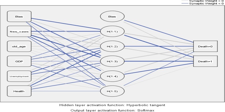
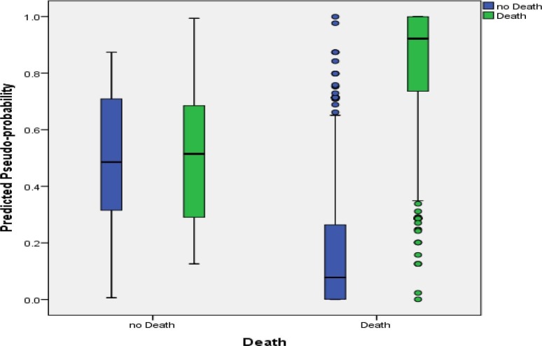
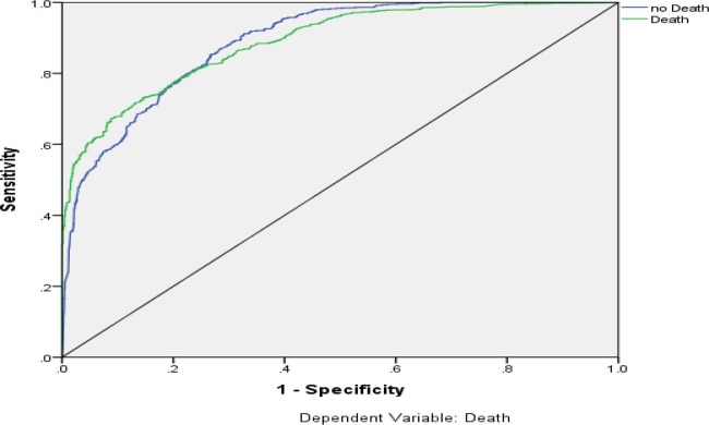
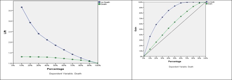
The total number of confirmed cases around the world was reported by WHO in different global regions; 3,415,174 in the Americas, 2,321,147 in Europe, 677,338 in Eastern Mediterranean countries, 392,674 in South-East Asia, 193,178 in Western Pacific countries and 145,287 in Africa [2]. This paper aims to compare and contrast two types of models, logistic regression, and artificial neural networks, used in analysis of the effects of the COVID-19 pandemic (see Fig. 1, Fig. 2, Fig. 3, Fig. 4 ).

Fig. 1.

Network diagram with five input nodes, one hidden layer with five nodes and two output nodes.

Fig. 2.

The predicted pseudo-probabilities.

Fig. 3.

The ROC curve is a diagram of sensitivity versus specificity. It illustrates the performance of classification concerning all potential cutoffs.

Fig. 4.

Lift and Gain charts for evaluating performance of classification models.

Methods

Data about COVID-19 pandemic was reported by WHO from 11th of January 2020 to 29th of May 2020 including 32 European countries. This data is correlated to other attributes such as, real GDP growth (annual percent change), per capita and for current international $, the Domestic General Government Health Expenditure, projected old-age dependency ratio per 100 persons, the percent of total labor force ages 15–24, unemployment is measured from a youth total (modeled ILO estimate) and new cases. The artificial neural networks and logistic regression models are appointed to analyze data.

Multilayer Perceptron (MLP)

Multilayer Perceptron (MLP) is the process which produced a prediction models for dependent variables. These are associated with one or more cases which are measured under the values of the predictors [10], [11].

Architecture (Multilayer Perceptron)

The Architecture of MLP is utilized to specify the network's structure. The MLP is consist of three layers of nodes; input, hidden and output layers [12], [13].

Hidden layers

The hidden layers contain of unobserved network nodes (units) that apply different transforms to inputs. Each of these hidden units are considered for the weighted sum as a function of the inputs. Then, the weights values from this activation function are specified by using the estimation algorithm [14]. The cases of network which contain the second hidden layer are considered as a function of the weighted sum from units given by the first hidden layer. Furthermore, this activation role is applied in two layers [15]. The considered activation function is applied to link the values of units in the succeeding layer with the weighted sums of units in a layer. The function in equation (1) is Hyperbolic tangent and the function in equation (2) is a sigmoid function.

$$\gamma \left(z\right)=\mathrm{t}\mathrm{a}\mathrm{n}\mathrm{h}(\mathrm{d})=({\mathbf{e}}^{\mathbf{z}}-{\mathit{e}}^{-\mathbf{z}})/({\mathit{e}}^{\mathbf{z}}+{\mathit{e}}^{-\mathbf{z}})$$ (1)

$$\mathrm{s}\left(\mathrm{z}\right)=\frac{1}{1+\mathrm{e}\mathrm{x}\mathrm{p}(-\mathrm{z})}$$ (2)

Output layer

The dependent variables as target are contained in output layers.

Logistic regression model (LRM)

Logistic regression model (LRM) is defined by transforming the linear regression equation with the sigmoid function in equation (2) [16].

The formula of LRM is as follow:

$$\mathrm{f}\left(\mathrm{z}\right)=\frac{1}{1+{\mathrm{e}}^{-\left({\beta }_0+{\beta }_1{\mathrm{x}}_1+\cdots +{\beta }_{\mathrm{n}}{\mathrm{x}}_{\mathrm{n}}\right)}}$$ (3)

The LRM used the sigmoid function to determine the value of y within the range (0 to 1) from a large scale.

Data analysis

Neural network (NN)

The information of the networks and the case processing summary of data which is used to build the NN model are illustrated in Table 1, Table 2 .

Table 1.

Summary of Case Processing.

		N	Percent
Sample	Training	2191	70.2%
	Testing	931	29.8%
Valid		3122	100.0%
Excluded		0
Total		3122

Table 2.

Network Information.

Input Layer	Covariates	1	New cases
		2	Projected old-age dependency ratio per 100 individuals
		3	Real GDP growth (annual percent change)
		4	Unemployment, youth total (% of total work force aged 15–24) (modeled ILO estimate)
		5	Domestic general government health expenses per capita, PPP (current international $)
Number of Units			5

The classification in Table 4 shows the overall percent is 85.5% of the training cases are correctly classified (see Table 3 ).

Table 4.

Classification.

Sample		Predicted
		no Death	Death	Percent correct
Training	no Death	248	252	49.6%
	Death	61	1599	96.3%
	Overall percent	14.3%	85.7%	85.5%
Testing	no Death	109	119	47.8%
	Death	20	714	97.3%
	Overall percent	13.4%	86.6%	85.6%

Dependent Variable: Death.

Table 3.

Summary of the Model.

Training	Cross Entropy Error	736.070
	Percent Incorrect Predictions	14.5%
	Stopping Rule Used	1 consecutive step(s) with no decline in errora
	Training Time	0:00:01.41
Testing	Cross Entropy Error	327.182
	Percent Incorrect Predictions	14.4%

Dependent Variable: Death.

a. The testing sample is the basis of error calculations.

Logistic regression

Logistic Regression model is considered with the death as a dependent variable and the following independent variables:

• 1. $X_1$is the projected old-age dependency ratio per 100 persons.
• 2. $X_2$is the real GDP growth (annual percent change).
• 3. $X_3$ is the unemployment, youth total (% of total work force aged 15–24) (modeled ILO estimate).
• 4. $X_4$is the Domestic general government health expenditure per capita.
• 5. $X_5$is the new cases.
• 6.The proposed regression model is given by:

$$\mathrm{P}\left(1\right)=\frac{{\mathrm{e}}^{\mathrm{Y}\text{'}}}{(1+{\mathrm{e}}^{\mathrm{Y}\text{'}})}$$ (4)

where,

Y' = 1.425–0.0256  $X_1$ + 0.0557  $X_2$ + 0.0403  $X_3$ + 0.000198  $X_4$ + 0.02467 $X_5$

Table 5 observes the odds ratio for the predictors and their 95% confidence intervals. Table 6, Table 7 show that the proposed model (LRM) is explained by the arguments.

Table 5.

Odds ratio for continuous predictors.

Predictors	Odds ratio	95% CI
Projected old-age dependency ratio Per 100 individuals	0.9747	(0.9553, 0.9945)
Real GDP growth (Annual percent change)	1.0573	(0.9929, 1.1258)
Unemployment, youth total (% of total work force aged 15–24) (modeled ILO estimate)	1.0411	(1.0156, 1.0673)
Domestic general government health expenses per capita, PPP (current international $)	0.9998	(0.9997, 0.9999)
New cases	1.025	(1.0215, 1.0285)

Table 6.

Summary of the Model.

Deviance R-Sq	Deviance R-Sq(adj)	AIC	AIC	BIC
27.58%	27.44%	2467.7	2467.8	2504

Table 7.

Tests of goodness-of-Fit.

Test	Degree of freedom	Chi Square	P-Value
Deviance	3116	2455.73	1
Pearson	3116	11879.86	0
Hosmer-Lemeshow	8	77.2	0

Since all p-values are less than 0.05, the proposed model has meaningful.

Conclusion

The spread of the COVID-19 pandemic worldwide has threatened people, the economy, and the lifestyles of all human beings. The aim of this study has been to evaluate the application of machine learning models (MLP) and the statistical model of logistic regression. Additionally, the research has compared the accuracy rate of machine learning models and the stated statistical model and given some statistical indicators concerning COVID-19. It has been revealed that the performance of MLP is better than LRM, as the classification accuracy rate was higher 85.6% against 80.8%, see Table 4, Table 9. Interestingly, the areas with a larger population show a tendency to have more cases than those with a smaller population. COVID-19 deaths among females have been revealed to have been higher than those among men in the UK and higher among people over 65 years of age.

Table 9.

Classification Table.

Observed			Predicted
			Death		Percentage correct
			no Death	Death
Step 1	Death	no Death	1148	139	89.2
		Death	460	1375	74.9
	Overall Percentage				80.8

a. The cut value is 0.5.

The classification in Table 4 shows that the overall percent of 85.5% of the sample cases of the study had been correctly classified. The model summary in Table 6 and the goodness of fit test in Table 7 show how much the proposed model (LRM) has been explained by the arguments. Table 8 shows that all p-values are less than 0.05; therefore, the proposed model (LRM) has had meaningful results.

Table 8.

The Wald Test.

The Source	DF	Chi-Square	P-Value
Regression	5	242.39	0.000
Projected old-age dependency ratio per 100 individuals	1	6.24	0.012
Real GDP growth (annual percent change)	1	3.02	0.082
Unemployment, youth total (% of total work force aged 15–24) (modeled ILO estimate)	1	10.12	0.001
Domestic general government health expenses per capita, PPP (current international $)	1	29.37	0.000
New cases	1	202.88	0.000

Data availability

No data were used to support the findings of this study.

Declaration of Competing Interest

The authors declare that they have no known competing financial interests or personal relationships that could have appeared to influence the work reported in this paper.