Astrocyte Regional Heterogeneity Revealed Through Machine Learning-based Glial Neuroanatomical Assays

Abstract

Evaluation of reactive astrogliosis by neuroanatomical assays represents a common experimental outcome for neuroanatomists. The literature demonstrates several conflicting results as to the accuracy of such measures. We posited that the diverging results within the neuroanatomy literature were due to suboptimal analytical workflows in addition to astrocyte regional heterogeneity. We therefore generated an automated segmentation workflow to extract features of glial fibrillary acidic protein (GFAP) and Aldehyde Dehydrogenase Family 1, Member L1 (ALDH1L1) labeled astrocytes with and without neuroinflammation. We achieved this by capturing multiplexed immunofluorescent confocal images of mouse brains treated with either vehicle or lipopolysaccharide (LPS) followed by implementation of our workflows. Using classical image analysis techniques focused on pixel intensity only, we were unable to identify differences between vehicle-treated and LPS-treated animals. However, when utilizing machine learning based algorithms, we were able to (1) accurately predict which objects were derived from GFAP or ALDH1L1 stained images indicating that GFAP and ALDH1L1 highlight distinct morphological aspects of astrocytes, (2) we could predict which neuroanatomical region the segmented GFAP or ALDH1L1 object had been derived from, indicating that morphological features of astrocytes change as a function of neuroanatomical location. (3) We discovered a statistically significant, albeit not highly accurate, prediction of which objects had come from LPS versus vehicle-treated animals, indicating that although features exist capable of distinguishing LPS-treated versus vehicle-treated GFAP and ALDH1L1 segmented objects, that significant overlap between morphologies exists. We further determined that for most classification scenarios, non-linear models were required for improved treatment class designations. We propose that unbiased automated image analysis techniques coupled with well-validated machine learning tools represent highly useful models capable of providing insights into neuroanatomical assays.

Introduction

Astrocytes undergo activation during brain injury through an ill-defined process known as gliosis. Classic neuropathological studies describe gliosis mainly through a histomorphological lens, characterized by eccentric displacement of the cell nucleus and accumulation of a large eosinophilic cytoplasm on hematoxylin and eosin stained tissue sections. Recent work focused on elucidating the molecular underpinnings of glial response to injury resulted in the promotion of a binary classification system of reactive gliosis denoted “A1” and “A2”, with so-called A1 astrocytes expressing pro-inflammatory and potentially harmful stimuli, whereas A2 reactive astrocytes, initially described in murine infarction models, manifest more protective roles (Liddelow & Barres, 2017; Liddelow et al., 2017). This classification system remains fluid, undergoing constant refinement as contemporary techniques and methodologies, such as single-cell RNAseq, add new information to our knowledge base. However, astrocytes exist in a unique three-dimensional space within the central nervous system (CNS), and their location is highly relevant to cellular function. This positional information disappears in single-cell RNAseq analyses and can only be obtained through neuroanatomical assays. Unfortunately, emerging techniques, such as single-cell spatial transcriptomic assays (Lein, Borm, & Linnarsson, 2017; Moffitt et al., 2016; Shah, Lubeck, Zhou, & Cai, 2016; Wang et al., 2018), are very costly and not broadly available amongst neuroscientists. Therefore, generating cost-effective neuroanatomical assays, which maintain the CNS positional information of astrocytes relative to their neural networks, remains the optimal approach to assess astrocyte reactivity in disease states.

A specific challenge of modern, quantitative, experimental neuroanatomy rests in converting unstructured, visual imaging data derived from microscopic images into structured, numerical data amenable to statistical hypothesis testing. Many astrocytic neuroanatomical assays in the scientific literature measure mean fluorescence intensity of GFAP or area of pixels above a specific value (for instance, see (Cao, Wang, Ren, & Zang, 2015; Feilchenfeld, Yücel, & Gupta, 2008; Javdani, Ghorbani, & Hashemnia, 2020; Luo, Xu, Yi, & Du, 2009; McKeever, 1992; Norden, Trojanowski, Villanueva, Navarro, & Godbout, 2016)). GFAP is typically used as a marker for gliosis due to its high expression in reactive astrocytes that are responding to CNS injury (Oberheim, Goldman, & Nedergaard, 2012; Sofroniew & Vinters, 2010). However, not all astrocytes express GFAP (Oberheim et al., 2012), especially astrocytes found in the gray matter, which makes it necessary to counterstain with anti-ALDH1L1 antibody in mice (Reemst, Noctor, Lucassen, & Hol, 2016). ALDH1L1 is a murine pan-astrocytic marker labeling the cell soma, but not all glial processes (Yoon, Walters, Paulsen, & Scarisbrick, 2017). Thus, GFAP and ALDH1L1 highlight different aspects of astrocytic morphology. Modern advances in computer vision and machine learning algorithms have given us the tools with which we can now extract a multitude of features from microscopic imaging data. Automated astrocyte segmentation analysis is not a new concept, however, advanced computational tools can allow us to analyze beyond the area of pixels above a specific intensity value (Zilles, Hajós, Kálmán, & Schleicher, 1991). By segmenting astrocytes from an image into numerous GFAP or ALDH1L1 positive “objects”, one can then extract numerical values that indicate object location, object pixel intensities, object shapes, as well as object textures from the original image.

In this study, we tested the hypothesis that astrocyte response to injury undergoes heterogenous morphological changes in different brain regions. To test this hypothesis, we developed an automated segmentation algorithm for both GFAP and ALDH1L1 immunostained mouse brain sections treated with vehicle or systemic lipopolysaccharide (LPS) to induce neuroinflammation. Lipopolysaccharide, the active ingredient of gram negative bacterial endotoxin, promotes CNS inflammation following peripheral administration and is a commonly utilized experimental model of sepsis-related systemic inflammation (Nemzek, Hugunin, & Opp, 2008). These images were captured on a laser scanning confocal microscope and subjected to our workflow to extract features characterizing shape, fluorescent intensity, and fluorescent texture. We then utilized a covariance matrix and the random forest-based Boruta algorithm to identify the most pertinent imaging features for classification, followed by cluster analysis and principal component analysis to evaluate the differences between reactive astrocytes and baseline astrocytes in three brain regions. We show that classification of segmented objects into reactive versus baseline astrocyte objects is inaccurate when our algorithms are trained on imaging data from one region and then used to attempt to predict objects from other neuroanatomical regions. This lack of generalizability to other regions underscores the notion that astrocyte morphological changes in response to injury occur as a function of anatomic location. We conclude that utilization of machine learning models developed to classify neuroanatomical images provides a highly insightful methodology to discover new processes by which astrocytes react to injury.

Materials and Methods

Experimental Animals

Procedures utilizing mice were performed in accordance with The Ohio State University Institutional Animal Care and Use Committee guidelines (protocol number: 2012A00000162-R1). Postnatal day 5 (P5) CD-1 mice (Charles River) from the same litter were used. Mice were selected from the litter and randomly assigned to receive the treatment (n = 5) or control (n = 5). Mice received a single dose of intraperitoneal injection (1 mg/ml) of Escherichia coli lipopolysaccharide (LPS) (Millipore Sigma, LPS from E. coli 0111:B4) in sterile saline or only sterile saline. Animals were sacrificed 3 hours after receiving the injection. All mice were anesthetized using a mixture of ketamine (100 mg/kg) and xylazine (10 mg/kg) in sterile saline. Mice were perfused transcardially, first with 10 mL phosphate-buffered saline (PBS), then with 5 mL 4% paraformaldehyde (PFA) (w/v) in pH 7.4 Phosphate buffer.

Tissue Processing

Brains were dissected and underwent post-perfusion fixation in 4% PFA (w/v) in pH 7.4 of 0.015M Phosphate buffer at 4°C overnight. Brains were transferred to 30% sucrose (w/v) in 0.015M Phosphate buffer at 4°C until equilibrated and optimal cutting temperature (OCT) embedded. OCT-embedded brains underwent cryosectioning (Microm HM 525, Microm Laboratories, Walldorf, Germany) coronally at 14 μm and were mounted onto a Vectabond-coated slide (Vector Labs SP-1800). Brain regions within the hippocampus dentate gyrus (DG) and Cornu Ammonis 1 (CA1), 2 (CA2), and 3 (CA3) were identified by reference markers in accordance with the stereotaxic mouse brain atlas (Franklin & Paxinos). Sections dried at room temperature for approximately 45 minutes and then placed in the −80°C freezer until further use.

Immunohistochemistry

Tissue sections were washed with 0.015M phosphate buffer containing 0.1% Triton X-100 (#02300221, MP Biomedicals, Solon, OH, USA) once for twenty minutes and then twice for five minutes at room temperature. Antigen retrieval was performed in 10mM citrate buffer (pH 6.0) for 30 minutes at 80°C. Sections were then blocked with 10% horse serum (#06750, Stem Cell Technologies, Vancouver, British Columbia, Canada), 1% Bovine Serum Albumin (BSA) (BP1605-100, Thermo Fisher Scientific, Waltham, MA, USA), and 0.015M Phosphate buffer containing 0.1% Triton X-100 for 2 hours at room temperature. After, sections were incubated overnight at 4°C with primary antibodies diluted in the same blocking solution. Table 1 contains primary antibodies descriptions. Sections were washed with 0.015M Phosphate buffer containing 0.1% Triton X-100 three times for five minutes. Secondary antibodies used were Alexa Fluor 488-conjugated goat anti-chicken secondary antibody (Molecular Probes, A-11039, Invitrogen, Carlsbad, CA, USA), Alexa Fluor 594-conjugated goat anti-MSIgG2b secondary antibody (Thermo Fisher Scientific, A-21145, Carlsbad, CA, USA), Alexa Fluor 647-conjugated goat anti-rabbit secondary antibody (Molecular Probes, A-21244, Carlsbad, CA, USA), and counterstained with DAPI (#D1306, Invitrogen, Carlsbad, CA, USA). All secondary antibodies were used at 1:1000 and incubated 2 hours at room temperature in the dark. Sections were washed with 0.015M Phosphate buffer containing 0.1% Triton three times for five minutes and coverslips were mounted with ProLong Gold Antifade Mountant (#P36934, Invitrogen, Eugene, OR, USA).

Table 1-.

Description of Primary Antibodies

Antibody	Source	Dilution	Species	Immunogen	RRID
Anti-ALDH1L1	OriGene (UMAB43)	1:300	Mouse monoclonal- IgG2b	Full length human recombinant protein of human ALDH1L1 (NP_036322) produced in HEK293T cell.	AB_2629053
Anti-GFAP	Abcam (AB134436)	1:100	Chicken polyclonal	Recombinant full length protein followed by boosts of native GFAP protein purified from bovine spinal cords	AB_2818977

Microscopy and Image Analysis

Fluorescent images were captured on a Carl Zeiss Axio Imager Z.1 with LSM700 confocal microscope with a motorized stage using 40x/1.3 numerical aperture Oil DIC objectives. A z-stack containing 3-4 images were separated by 2.60-5.20 μm Z-steps depending on region of interest. Images were taken at 40x magnification with a pinhole of 1 Airy unit, scan speed of 8, resolution of 1512 x 1512, and pixel resolution of 6.3983pixels/μm. For each mouse, 9-12 representative images were taken in the hippocampus, caudoputamen, and the retrosplenial neocortex at the dorsal aspect and along the longitudinal fissure. Images from all regions were obtained from the same tissue section. All image acquisition parameters (eg., microscope laser power and gain) were identical in all confocal image acquisitions. Images were captured and saved as .czi files and then opened in FIJI. Z-stacks were average intensity projected in FIJI (v1.0, RRID:SCR_002285) and saved as .tiff files for importation into Rstudio. Following image acquisition, multiple image segmentation workflows were developed within Rstudio to optimize the segmentation process with images in the hippocampus.

Linear Modeling and Traditional Florescent Intensity Analysis

One image from each region and treatment was randomly selected and loaded into R. Channels were split for the biomarkers discussed above. Using 20% of the pixel values from each image with a random sample, pixel intensity values were plotted to determine if there was a difference in colocalization between ALDH1L1 and GFAP. Next, a boxplot of the mean pixel intensity value for each biomarker was generated based on the region. Linear models were applied to predict GFAP from each region utilizing the GFAP-ALDH1L1 pixel intensity values as predictors. Packages used: EBImage (Pau, Fuchs, Sklyar, Boutros, & Huber, 2010), ggplot2 (Wickham, 2016), stats (R Core Team, 2019).

Automated Object Segmentation and Validation

R is an open source software commonly used for statistical computing and graphics generation, and was utilized through the Rstudio IDE (version 3.6.1, RRID: SCR_000432). Through R, it is possible to create workflows with installed packages that automatically follow the steps outlined in the process drastically reducing time for analysis. Images were loaded, astrocytes were segmented, and 89 variable features for every segmented object was extracted. Segmentation methods tested in this study include Otsu thresholding, k-means, and WEKA segmentation and their workflows are described below.

OTSU Thresholding -

Thresholding by neighboring pixel intensity values is a simple and classical method in astrocyte segmentation (Zilles et al., 1991). However, we sought to determine if a more basic method was superior compared to other supervised and unsupervised methods. We therefore generated the image segmentation workflow presented in figure 3. First, images were loaded into Rstudio using the EBImage package and channels separated for each secondary antibody. Each image is transformed into a grayscale image and a median filter applied, reducing noise while preserving the object’s edges (in this sense, an “object” represents a geographic area showing positive signal relative to background, as such representing a cell body or glial process) (Poostchi, Silamut, Maude, Jaeger, & Thoma, 2018). Application of a grayscale function to the image permitted rapid thresholding to a binary image via the Otsu function. Next, in these binary images each pixel obtains a value of the integer 0 or 1. We used Otsu thresholding in this application, which calculates the optimal threshold based off a bimodal histogram and neighboring pixel intensities (Poostchi et al., 2018). Next, we applied the Self Complementary Tophat algorithm, a feature within EBImage permitting morphological operations on a binary image, to determine if pixels of a specified width based on a Gaussian kernel will be closed utilizing the intensity level near neighboring pixels from the foreground (Oleś, Pau, Smith, Sklyar, & Huber, 2019). Lastly, we applied a segmented outline to the original image and visually validated how well the segmented object included the glial cell compartments (Roeder, Cunha, Burl, & Meyerowitz, 2012). In some images, a gamma correction filter was applied to reduce additional noise due to distinctions in the background luminance level. Gamma correction was applied before converting the image to grayscale. The complete image analysis workflow is delineated in figure 3 and code is found in supplemental materials. Packages used: EBImage (Pau et al., 2010).

Figure 3. Otsu Segmentation Workflow.

Immunofluorescence imaging was used to determine labeling of astrocytes with GFAP and ALDH1L1. To evaluate accuracy (a1), specificity (a2), and sensitivity (a3), segmented masks were evaluated against two ground truth images. Otsu outperformed the other segmentation methods. The Otsu workflow is described in b and c. Images were average projected in FIJI and loaded into R studio. Separate the channels into GFAP positive and ALDH1L1 positive labeled astrocytes (b1/c1). Create a grayscale image with pixel intensities from 0-255 (b2/c2). Apply filter and Otsu threshold to reduce the gray-level image to a binary image with intensities 0 or 1 (b3/c3). Process image to fill holes between pixels of a specified distance. Apply segmented boundary to original image and ensure object was properly segmented. Apply gamma correction as needed to reduce background luminance levels. Compute features of each object to extract morphological and textural features for analysis between conditions and anatomical regions of interest (b4/c4). (d1)- 94.45% accuracy of random forest model predicting ALDH1L1 and GFAP segmented objects obtained from the hippocampus of vehicle-treated mice (p < 2.2 x e⁻¹⁶ over the NIR). (d2)- Random forest model created with GFAP vehicle-treated objects from all regions with overall accuracy of 79.26% and balanced accuracy of 94.49%, 78.95%, 75.72% for the hippocampus, neocortex, and caudoputamen, respectively. Significance is based on calculating the probability that the accuracy elicited from the model is higher than the NIR. (d3)- Random forest model created with ALDH1L1 vehicle-treated objects from all regions used to predict the region in which objects originate. Overall accuracy is 84.07%. Balanced accuracy is 93.32%, 83.84%, 85.73% for hippocampus, neocortex, and caudoputamen respectively. (e1-e3)- Average of categories for Gini Importance in random forest models displayed in d1-d3 respectively. Pixel intensity features had the highest importance in each model. Specific model details found in supplemental table 2.

K-means segmentation -

In addition to performing unsupervised thresholding with Otsu, we also conducted k-means analysis to segment objects based on pixel intensity (Goceri et al., 2017). Images were loaded into R and a dataframe was generated with columns corresponding to the three biomarkers utilized (DAPI, GFAP, and ALDH1L1). Data for each image was center-scaled. Using the k-means function in the stats package, the dataframe was clustered based on 3 groups. Three mask images were created based on k = 1, k = 2, k = 3. An important caveat to consider is that a random row is selected when beginning the cluster analysis for each image so in some images k = 1 may indicate GFAP and ALDH1L1-positive objects but in a separate image k = 1 may highlight the segmented background. Following the generation of the masks, a watershed function is applied to separate fused objects and then the border applied to the original GFAP and ALDH1L1 combined image to determine how well the positive objects were segmented. Packages used: EBImage (Pau et al., 2010), stats (R Core Team, 2019)

WEKA segmentation -

In determining the best segmentation workflow, we also utilized the supervised learning method Waikato Environment for Knowledge Analysis (WEKA), available in FIJI. Compared to the previously described image segmentation techniques, a user must create classes and manually segment objects for the model to train. Images were loaded into FIJI and biomarker channels merged. Next a small region of the image was selected (~800 x 600 pixels) and copied into a new image file. The WEKA plugin was loaded, and 4 classes were created (GFAP; GFAP & ALDH1L1; DAPI; and background). Objects were manually segmented by an expert annotator and classified into these group. Next, the classifier was trained and generated a new segmented result and probability map. After saving the classifier, new images were loaded and underwent segmentation with the trained WEKA model.

Segmentation Validation -

Validation of the workflow was conducted on two ground truth images (one vehicle-treated and one LPS-treated image from the hippocampus) generated by the first author. Biomarker channels were separated for the generation of the ground truth. Performance of OTSU segmentation was calculated with ALDH1L1 and GFAP segmentation separated while the ground truth biomarker channels were merged when determining the accuracy of k-means and WEKA.

Biomarker and Region Evaluation

Biomarker morphologic evaluation was carried out within R to identify if there were inherent differences between segmented GFAP-positive and ALDH1L1-positive objects. GFAP and ALDH1L1 segmented object data from the hippocampus of vehicle-treated mice were utilized to troubleshoot the original workflow. Data was loaded to R and center-scaled together. Models were generated by random sampling of 70% of the objects for training data and tested on the remaining 30% of objects. Model performance evaluation was tested using the accuracy of the model predicting data biomarker against the no information rate.

Evaluation of both biomarkers within each region was tested next to determine if each biomarker provided insight to the regions studied. Extracted data from vehicle-treated animals from the hippocampus, neocortex, and caudoputamen were loaded into R and center-scaled.

Following this, models were generated to determine if reactivity state of segmented objects could be identified using extracted feature information (i.e., baseline astrocyte versus reactive astrocyte). Machine learning methods include random forests, support vector machines, and multi-layer perceptron (MLP) and performance of the models are included in supplemental tables 3–5. Models were created using 70% training data solely of region-specific objects and tested on the remaining 30% of objects. Modeling performance to predict region of the test data was evaluated based on the accuracy of each region over the no information rate (Bluemke et al., 2020). No external test set was used for statistical reporting. Following the optimization of these models using performance evaluation tools, these models were applied to other regions to determine if they could predict the reactivity state of the segmented objects. Packages used: randomForest (Liaw & Wiener, 2002), caret (Kuhn, 2019), RSNNS (Bergmeir & Benítez, 2012).

Extracted Variable Importance and Redundancies

To determine the drivers of variation between each biomarker and region, we evaluated feature importance by implementing random forests and principal component analysis (PCA). Utilizing objects from the hippocampus, feature importance in the random forest was computed using the Boruta package to identify how well each variable performed over the generated shadow feature (Kursa & Rudnicki, 2010). The Boruta algorithm works by shuffling features and comparing the importance of the shuffled features to the original features. Referred to as shadow features, the random forest will run the model with both the original feature and the shadow feature. During the iterations, the Boruta function compares the performance of the original feature to the shadow feature. If instances emerge where the original feature underperforms or is similar to the shadow features, such a feature would be deemed unimportant in this assay and subsequently removed from downstream analysis. Due to the large number of variables, we sought to identify correlated features to reduce redundancies by generating a correlation plot (data not shown). Variables chosen were two florescence intensity values, two shape measurements, and eight pixel texture features that described the texture of the whole object and comparison of neighboring pixel values. Definitions of each measure are included in supplemental table 1. A principal component analysis (PCA) was utilized next to reduce dimensionality of data and identify the variable drivers of variance of data. Variable drivers are visualized by eigenvector graphs. Packages used: randomForest (Liaw & Wiener, 2002), corrplot (Simko, 2017), MASS (Venables & Ripley, 2002), factoextra (Kassambara & Fabian, 2019).

Unsupervised Object Clustering

Unsupervised clustering was performed to determine object subclasses within each region and biomarker. Data from objects extracted from the LPS-treated mice in each region was loaded into R. In order to identify clusters of objects, we performed an unsupervised clustering procedure using the k-means algorithm. Other clustering methods utilized were k-medoids (Maechler, Rousseeuw, Struyf, Hubert, & Hornik, 2019), density-based spatial clustering of application with noise (DBSCAN) (Hahsler, M., Piekenbrock, M., Doran, D., 2019), ordering points to identify the clustering structure (OPTICS) (Hahsler, M., Piekenbrock, M., Doran, D., 2019), and a distribution-based method (Scrucca, Fop, Murphy, & Raftery, 2016). Using the NbClust function (Charrad, Ghazzali, Boiteau, & Niknafs, 2014), we determined the optimal number of clusters for each biomarker in each region. However, when the clusters were k = 3 or less, the clusters grouped meaningful objects into one cluster which limited analysis. Therefore, using the silhouette method, the optimal number of k-means clusters were determined and provided clusters with distinct morphologies of biomarkers in most regions.

To ensure the clusters determined by the silhouette method were meaningful, we performed internal clustering validation to compute the distance between objects and their respective clusters. We performed a permutation analysis to implement the cluster.stats() function call in R and evaluated the average distance between clusters, the average distance within clusters, and the within cluster sum of squares. Figure 8 discusses our workflow for this analysis. This permutation was repeated 1000 times, which permits identifying significance scores of up to 10⁻² (represented as 10⁻² due to being an estimate obtained using random sampled permutations (as described by (Knijnenburg, Wessels, Reinders, & Shmulevich, 2009))).

Figure 8. Clustering is Meaningful.

To determine the optimal number of clusters using 30 different clustering techniques, we utilized the NbClust package in R. In the GFAP LPS hippocampus objects, the optimal number was 3 clusters (a), but when running multiple iterations, cluster size varied and objects with distinct morphological profiles were grouped into one cluster further limiting our analysis (b; compare cluster designation to Figure 7 a1). Using the silhouette method (c) we determined the optimal number of clusters and ran a permutation analysis (d) to determine if our clusters were distinct compared to randomly assigned clusters. After 1000 iterations, the lack of overlap in the average distance between or within clusters and the within cluster sum of squares suggests the probability of this occurring due to chance as p < 10⁻² (e).

To determine the accuracy of cluster predictions, random forests and support vector machines were applied with the LPS data for each biomarker and region and the balanced accuracy for each subclass was calculated. P-values were calculated with the predictive accuracy compared to the no information rate. MLP was not utilized because support vector machine and random forest models had high accuracy at cluster prediction. Due to the support vector machine model having higher balanced accuracy for each subclass and overall accuracy, these models were used to predict the vehicle objects cluster designation. Comparison of object clusters was performed by the first author (not blinded to treatment information) identifying at least five objects per mouse from both treatments and every cluster within regions ensuring predicted object clusters were visually similar. Clusters showed very little overlap in the PCA (data not shown) and t-SNE plots colored based on cluster designation. Visualizing high-dimensional datasets with t-SNE allows for readers to appreciate similar data being plotted together and the ratio of objects in each cluster overall. Packages used: MASS (Venables & Ripley, 2002), factoextra (Kassambara & Fabian, 2019), caret (Kuhn, 2019), Rtsne (Krijthe, 2015), dbscan (Hahsler, M., Piekenbrock, M., Doran, D., 2019), cluster (Maechler et al., 2019), mclust (Scrucca et al., 2016), NbClust (Charrad et al., 2014)

Cluster Modeling with Linear Discriminant Analysis and Random Forest

Following cluster designation, dimensionality reduction with linear discriminant analysis was utilized to visually understand the overlap between objects from vehicle-treated mice and LPS-treated mice. Coefficients from the linear discriminant analysis were computed to determine feature importance in classifying objects’ reactivity. The region-specific random forest models from figures 5 and 6 (a1–c1) were applied to the objects in each cluster designation and accuracy and statistical significance comparing the no information rate was calculated. A separate random forest was created with only objects in each cluster designation as well with 70% training and 30% test set to evaluate performance when looking at a smaller dataset with similar objects. Packages used: randomForest (Liaw & Wiener, 2002), MASS (Venables & Ripley, 2002), caret (Kuhn, 2019).

Figure 5. Regionalization Predicting Activation and Eigen Vectors Showing Drivers of Variation of GFAP Segmented Objects.

Random forests models were created with 12 variables to predict reactivity state of segmented objects from one region. Models were applied to other regions and evaluated on performance of accurate prediction of reactivity state. Random forest models were accurate at only predicting object reactivity state in their regions (a1-c1), indicating a heterogenous response to inflammation (see supplemental table 3 for model performance statistics). To identify the drivers of variance between vehicle segmented objects and LPS segmented objects, a PCA was generated and eigenvectors calculated. (a2/b2) Vehicle segmented objects from the hippocampus and neocortex placed higher importance on shape features (area and perimeter) and lower importance on pixel intensity. In contrast, LPS segmented objects placed higher importance on pixel intensity and lower importance on shape features (a3/b3). In both vehicle segmented and LPS segmented objects from the caudoputamen, the highest driver of variance was Haralick features.

Figure 6. Regionalization Predicting Activation and Eigen Vectors Showing Drivers of Variation of ALDH1L1 Segmented Objects.

Random forests models were created with 12 variables to predict reactivity state of segmented objects from one region. Models were applied to other regions and evaluated on performance of accurate prediction of reactivity state. Random forest models had higher accuracy at predicting object reactivity state in their specific regions (a1-c1), however, models from the hippocampus and caudoputamen were statistically significance at predicting one another’s activation state indicating a similar response to inflammation (see supplemental table 3 for model performance statistics). To identify the drivers of variance between vehicle segmented objects and LPS segmented objects, a PCA was generated and eigenvectors calculated. (a2/b2) Vehicle segmented objects from the hippocampus and neocortex placed higher importance on shape features (area and perimeter). In contrast, LPS segmented objects placed higher importance on pixel intensity (a3/b3). In vehicle segmented objects from the caudoputamen (c2), the highest driver of variance was pixel intensity while LPS segmented objects (c3) placed higher importance on shape.

Machine learning tools: PCA and LDA analyses and graphics were generated utilizing unique scripts and the MASS (Venables & Ripley, 2002), factoextra (Kassambara & Fabian, 2019) and ggplot2 packages within R. Feature detection was done utilizing the Boruta package (Kursa & Rudnicki, 2010). Machine learning algorithms were generated utilizing the caret (Kuhn, 2019), e1071 (Meyer, Dimitriadou, Hornik, Weingessel, & Leisch, 2019), randomForest (Liaw & Wiener, 2002) and doParallel (Microsoft Corporation & Weston, 2019) packages in R. Machine learning decision importance was extracted utilizing the above packages and rminer package (Cortez, 2010).

Results

Classical Image Analysis Techniques Do Not Capture Neuroanatomical Reactive Glial Heterogeneity

Classic image analysis methods evaluating inflammation generally interrogate the mean fluorescence pixel intensity of GFAP, the percent area of positive pixels above a threshold, or colocalization with another biomarker (Cao et al., 2015; Feilchenfeld et al., 2008; Javdani et al., 2020; Luo et al., 2009; McKeever, 1992; Norden et al., 2016). As astrocytes show morphological heterogeneity and GFAP immunolabeling represents an insensitive test to astrocyte identity unable to label all astrocytes (Lee, Su, Messing, & Brenner, 2006), we additionally stained with ALDH1L1 in the same section due to ALDH1L1’s increased sensitivity to astrocyte identity (Cahoy et al., 2008; Neymeyer, Tephly, & Miller, 1997). Representative images of vehicle and LPS-treated mice from the hippocampus are displayed in figure 1. Observed in the bottom right corner of a2 (figure 1, white arrowhead), reactive astrocytes are seen and appear visually different from the astrocytes in a1. From these images, a random sample of 20% of the objects was performed and the pixel intensity of each biomarker displayed as a scatter plot (figure 1, a3/a4). Note that for the most part, the pixel intensity scatterplot shows little overlap between the two markers, underscoring the fact that these two biomarkers label distinct aspects of the cell (note that in randomly selected scatter plots from all regions, displays a rough “L-shape” indicating that high expression of one biomarker does not often show high expression of the other biomarker within the same pixel (data not shown for neocortex and caudoputamen)). We next tested if the arithmetic mean of GFAP or ALDH1L1 pixel intensity was distinct between the groups and no statistical significance in either biomarker was noted when comparing vehicle to LPS-treated samples (GFAP (b1): Hippocampus- p = 0.39; Neocortex- p = 0.47; Caudoputamen- p = 0.41; ALDH1L1 (b2): Hippocampus- p = 0.44; Neocortex- p = 0.43; Caudoputamen- p = 0.82, T-test). We then generated a linear model where we used ALDH1L1 pixel intensity and treatment (i.e., vehicle versus LPS) as predictor variables and GFAP as a response variable for each anatomical region. These linear models were unable to accurately predict GFAP pixel intensity (Hippocampus- p = 0.36; Neocortex- p = 0.9; Caudoputamen- p = 0.22). In summary, these data indicate that classical methods such as these do not capture differences between images obtained from vehicle and LPS-treated mice and fail to reject that LPS causes a change in astrocyte fluorescence expression with the biomarkers ALDH1L1 and GFAP.

Figure 1. Traditional Image Analysis Methods.

Immunofluorescence imaging was used to determine labeling of astrocytes with GFAP and ALDH1L1. Images from vehicle and LPS-treated mice were used to determine the pixel intensity and colocalization of GFAP and ALDH1L1. A scatterplot was generated with a random sample of 20% of the data from each region (data shown only for hippocampus, a1/a2). There is no apparent difference in the colocalization of GFAP and ALDH1L1 pixel intensity in vehicle or LPS-treated mice (a3/a4). Similar plots were observed for neocortex and caudoputamen. Next, evaluation of the mean fluorescence intensity was calculated for GFAP (b1) and there was no significant increase between the vehicle and LPS (Hippocampus- p = 0.39; Neocortex- p = 0.47; Caudoputamen- p = 0.41). ALDH1L1 mean pixel intensity was calculated next (b2) and there was no difference between the control and treated groups (Hippocampus- p = 0.44; Neocortex- p = 0.43; Caudoputamen- p = 0.82).

Automated Segmentation of Astrocyte Objects Labeled with ALDH1L1 and GFAP Reveal Heterogeneity

Having shown that traditionally quantifiable metrics were unable to distinguish images from animals undergoing neuroinflammation when compared to vehicle-treated animals, we decided to test the extent to which automated segmentation of astrocyte objects would be capable of proper image classification. From each sample of control group (n=5) and LPS (n=5), three regions of interest, 9-12 images from each mouse in each region, and over 300 images were acquired at 40x magnification in confocal Z-steps, representing a total of 7.99 GB of data. Images were obtained from each region on the same tissue section (always the ipsilateral side on the hippocampus and caudoputamen and bilaterally when capturing images from the neocortex) to ensure they underwent the same immunohistochemical conditions. These data were simplified by creating average intensity projections from each confocal Z-stack image. Representative images of each region are displayed in figure 2. Our goal was to develop a time efficient, objective segmentation method providing insight into morphological changes astrocytes undergo as a function of LPS treatment. Despite morphological differences between vehicle and LPS-treated groups in the sample images shown in figure 2, unequivocal discernment of the image features upon which these observations are based were unusually challenging. Within the images from the hippocampus and neocortex, the processes appear more arborized than the caudoputamen. Furthermore, an abundance of ALDH1L1 in the caudoputamen is noted when compared to the images of the hippocampus and neocortex. Due to the emerging field of automated biomedical image analysis, we applied three image segmentation methods to ensure we used the most accurate technique in our approach. These methods include two unsupervised techniques (Otsu thresholding and k-means) and one supervised approach (WEKA). Although our dataset was large, deep learning segmentation was not attempted due to the small number of training images in our dataset, with some neural network architectures using over 1000 ground truth images to train their segmentation model (Suleymanova et al., 2018). Segmentation performance was calculated using two ground truth images (one vehicle-treated and one LPS-treated from the hippocampus) using both biomarkers. Accuracy, specificity, and sensitivity for each method are shown in figure 3 a1–a3. Otsu thresholding represented the most accurate, simple, specific, and sensitive technique capable of generating segmented masks and outperformed k-means and WEKA segmentation.

Figure 2. Image Capture Methodology.

Images were captured at 40x magnification of three regions on the same coronal section of 5 vehicle-treated and 5 LPS-treated mice. Images in the caudoputamen and hippocampus were obtained ipsilaterally while the neocortex images were captured bilaterally on the same section. Representative images of each region are shown (a1/a3-b1/b3). 9-12 images were captured per mouse in each region with 152 images total per condition.

Following successful segmentation, the computeFeatures function call in Rstudio was utilized to extract from each object its morphological, fluorescence intensity, and fluorescence textural features (also known as Haralick features (Haralick, Shanmugam, & Dinstein, 1973)). Supplemental table 1 delineates all the variables obtained from Rstudio’s computeFeatures function that were implemented in our workflow. Our workflow generates a data table containing each numbered segmented object in rows, with each feature extracted by the computeFeatures function call as a column. Such rectangular data tables are easily modified within the Rstudio IDE for downstream statistical analysis. Although 89 features are extracted in the computeFeatures function call, several features are highly correlated to each other, and utilize marginally different scales calculating Haralick features (Oleś et al., 2019; Vrbik et al., 2019). Subsequent to object data extraction with computeFeatures, another image was produced with the corresponding object number from the compute features file on segmented objects to allow for classification of ALDH1L1-positive and GFAP-positive components and allow for cluster analysis. Following this process, the image segmentation workflow was confirmed visually on both channels from every image before redoing the segmentation process with a different gamma correction if needed. The GFAP and ALDH1L1 positive objects segmentation code has been included in Supplemental Materials.

We next sought to determine if the GFAP and ALDH1L1 biomarkers label different astrocyte morphologies. In order to test this, we utilized the morphological data from the segmented objects of GFAP or ALDH1L1 stained slides to determine if we could train a classification algorithm to easily identify if an object had been either a GFAP labeled object or an ALDH1L1 labeled object. First, the data tables from ALDH1L1 and GFAP from the hippocampus dataset were randomly split- 70% of the data into a training set, and 30% of the data into a test set. In each set, ALDH1L1 or GFAP were the class labels of each object. Second, a random forest was trained to predict the class label (either ALDH1L1 or GFAP) based on the extracted features of each object. Once trained, this random forest accurately labeled objects as GFAP or ALDH1L1 with 94.45% accuracy (figure 3 d1) on the test data (no information rate (NIR) = 50.38% and the probability that accuracy was greater than the NIR occurred by chance was p < 2.2 x 10⁻¹⁶). We conclude that the morphological features outlined by the GFAP and ALDH1L1 biomarkers are distinct in baseline brain sections, likely due to the known differences in subcellular localization in astrocytes for these two biomarkers.

We next sought to determine the extent to which the biomarkers used to label astrocytes provided insight to regionalization. A random forest was trained with vehicle-treated objects from each region based on segmented object features from either GFAP or ALDH1L1. The GFAP model had an overall accuracy of 79.26%, NIR of 47.70%, and a significance of p < 2.2 x 10⁻¹⁶ on successfully predicting the region over the no information rate (figure 3 d2). Balanced accuracy for each region was 94.49%, 78.95%, and 75.72% for hippocampus, neocortex, and caudoputamen, respectively. The ALDH1L1 model had an overall accuracy of 84.07%, NIR of 39.01%, and a significance of p < 2.2 x 10⁻¹⁶ on successfully predicting the region over the no information rate (figure 3 d3). Balanced accuracy for each region was 93.32%, 83.84%, and 85.73% for hippocampus, neocortex, and caudoputamen, respectively. The variable importance for each model described in figure 3 d1–d3 are displayed in figure 3 e1–e3 (highest importance was place on pixel intensity values). Interpreting the results in toto, we posit that random forest shows strong predictive capacity to distinguish the GFAP or ALDH1L1 biomarker label, and to determine the neuroanatomical region from where the segmented object was derived from. We conclude GFAP and ALDH1L1 highlight different aspects of astrocytes, and that astrocytes morphological features, although showing significant overlap between regions, change as a function of neuroanatomical location. We further conclude that hippocampal astrocytes show highly unique morphological features relative to other brain regions since we were able to most accurately delineate the region in these astrocytes in both GFAP and ALDH1L1 experiments.

Regional Morphological Heterogeneity in Reactive Astrogliosis Can be Revealed through Random Forest Modeling

With 89 variables computed for every segmented object and the number of segmented objects obtained from each image ranging from 10-950 objects, it was imperative to reduce the features so that we could simplify our downstream statistical workflows. To this end, we next sought to identify key features utilized by the random forest to predict astroglial reactivity through implementing the Boruta algorithm. Although all features tested defeated their shadow features (data not shown), the fluorescence intensity values showed higher importance for prediction of objects as coming from either LPS or vehicle-treated images. A random forest model was trained to predict treatment (vehicle or LPS) using the full features dataset (defined in supplemental table 1) from the hippocampus from either GFAP-labeled or ALDH1L1-labeled objects. These random forest models showed 78.28% accuracy at predicting the treatment class label (i.e., class label = vehicle or LPS) of GFAP labeled objects and 78.69% accuracy on ALDH1L1 objects, each showing statistical significance (p < 2.2 x 10⁻¹⁶). However, when testing these models on objects from other regions, the GFAP hippocampus model (figure 4 a) performed with an accuracy of 49.80% and 52.65% on neocortex and caudoputamen GFAP segmented objects, respectively, which were not significantly different from the NIR in the confusion matrix (p = 1). This failure to properly classify GFAP objects as vehicle or LPS-treated objects indicates that the morphological features characteristic of hippocampal GFAP objects are not generalizable to the caudoputamen or neocortex. We performed similar analyses with the ALDH1L1 model, where the accuracies were 41.71% and 58.09% predicting the reactivity states of neocortex and caudoputamen ALDH1L1 objects, respectively (p = 1 and p < 2.2 x 10⁻¹⁶).

Figure 4. Feature Reduction and Random Forest Models Predicting Reactivity State.

Using objects extracted from the hippocampus, a random forest was generated to perform the Boruta algorithm to identify key variables. The hippocampal random forest reactivity model (a) was applied to the full compute.features hippocampal test set, neocortex, and caudoputamen and evaluated on performance of accurate prediction. The GFAP hippocampal model had an accuracy of a 78.28% on hippocampal objects and a significance of p < 2.2 x e⁻¹⁶. Applied to the neocortex and caudoputamen, it had an accuracy of 49.80% and 52.65%, respectively (p = 1). The ALDH1L1 hippocampal model had an accuracy of 78.69% (p < 2.2 x e⁻¹⁶) on hippocampal test data. On neocortex and caudoputamen objects, the accuracy was 41.71% and 58.09% (p = 1 and p < 2.2 x e⁻¹⁶, respectively). Twelve variables were selected based on a correlation plot of all features and other studies performing image analysis with Haralick features. New random forest models created with hippocampal objects identified each feature with Boruta algorithm (b) for importance. Correlation plot of twelve variables (c) used in the model based on 10000 objects from the hippocampus with each biomarker. Dark blue indicates high positive correlation, dark red indicates high negative correlation. Model performance listed in supplemental table 3.

Next, the number of features was reduced by removing redundant features validated and based on the Boruta algorithm (figure 4 b), correlation plot analysis (figure 4 c), and by selecting features used by other investigators published in the biomedical image analysis literature (Brynolfsson et al., 2017; Vrbik et al., 2019). Selected Haralick features were chosen based on their ability to describe the texture of the entire segmented object in addition to describing the texture of neighboring pixels. This trimmed feature table contained two intensity features (mean intensity and first percentile intensity of the object), two shape features (area and perimeter), and eight texture features (con, idm, f12, asm, cor, ent, f13, and var, see supplemental table 1 for glossary- definitions highlighted). These twelve features are the only variables included during analysis for the remainder of the text. Within these selected features, a new random forest was trained for each biomarker and the Boruta algorithm was performed to evaluate the importance of each variable at classifying treatment class. A correlation plot of the selected variables identified a strong positive correlation between mean pixel intensity with the 1^st percentile intensity value, a strong positive correlation between the perimeter and area for both biomarkers, and a negative correlation between homogeneity of each object with the entropy (figure 4 c).

New reduced feature random forests, support vector machines, and MLP neural network were evaluated on the region in which it was generated. Model performance statistics are listed in supplemental tables 3–5 with the random forest models performing at the same or marginally better over the other methods. Machine learning classification models were created with the same segmented objects from Figure 4 (a), however, using only the reduced features as described above. The hippocampus GFAP model (figure 5 a1) had an accuracy of 67.48% while the ALDH1L1 model (figure 6 a1) had an accuracy of 73.14% when evaluating the test data (p < 2.2 x 10⁻¹⁶ for both). However, similarly to the random forests discussed previously, the GFAP hippocampal model was a poor predictor of the activation state of neocortex and caudoputamen objects (49.02% and 51.54%, respectively, p = 1 and 0.9995) while the ALDH1L1 hippocampal model was a poor predictor of neocortex objects (41.84%). In contrast, the hippocampal ALDH1L1 model accurately predicted the activation state of caudoputamen objects with 57.33% accuracy and statistical significance of p < 2.2 x 10⁻¹⁶.

Next, region-specific models were generated for the neocortex and caudoputamen. The neocortex model showed accuracies of 63.78% for GFAP (figure 5 b1) and 64.48% for ALDH1L1 (figure 6 b1), respectively (both significantly different from NIR with p < 2.2 x 10⁻¹⁶). Similarly, the caudoputamen random forest model showed accuracies of 63.81% for GFAP (figure 5 c1) and 70.59% for ALDH1L1 (figure 6 c1), (both significant at p < 2.2 x 10⁻¹⁶). These region-specific models were used later in analysis as illustrated in figures 9 and 10 f. In summary, when training a classifier algorithm to detect reactive versus baseline astrocytes, these classifiers require neuroanatomical localization context. From these data we can conclude that (1) significant morphological overlap exists between the baseline and inflamed astrocytes due to the relatively low, albeit highly statistically significant, accuracy in predicting the treatment class label, and (2) that astrocytes show distinct morphological pattern changes based on the neuroanatomical region.

Figure 9. Evaluation of Hippocampal Astrogliosis Clusters in GFAP.

Within the hippocampus, although there were five clusters predicted with the silhouette method, only Cluster 1 and Cluster 3 included identifiable processes. Cluster 1 LPS objects are colored indigo in the t-SNE plot (a). Gray line intersection indicates the location of the LPS object (c) shown in relation to other objects within the cluster in the t-SNE plot. Generally, these were large objects (~5 μm) and contained the cell body and long processes (b/c). Cluster 3 objects are colored in teal in the t-SNE plot (a). These objects were generally segmented possesses in cross section or a small portion longitudinally (~ 1 μm, b). When generating a LDA, there is a large overlap between the vehicle and LPS objects (d). The most important variables classifying vehicle versus LPS-treated objects were fluorescent intensity and texture features (e). Although there is large overlap between the objects as seen in the LDA density plot, the random forest from figure 5 (a1) was able to predict with high accuracy the reactivity of objects (Cluster 1- Region Specific (RS): 73.53%; Cluster Specific (CS): 72.75%. Cluster 3- RS: 66.62%; CS: 65.69%).

Figure 10. Evaluation of Hippocampal Astrogliosis Clusters in ALDH1L1.

In ALDH1L1 objects, only Clusters 1, 4, and 6 contained recognizable objects. Gray line intersection indicates the location of the LPS object (c) shown in relation to other objects within the cluster in the t-SNE plot (a). Examples of vehicle and LPS objects are shown (b/c). Similarly to the GFAP labeled objects, the LDA shows a high overlap of vehicle and LPS segmented objects but the random forest was highly accurate and every model had a significance of p < 2.2 x e⁻¹⁶. Accuracies are Cluster 1- Region Specific (RS): 78.25%; Cluster Specific (CS): 73.61%; Cluster 4- RS: 88.45%; CS: 79.91%; Cluster 6- RS: 74.46%; CS: 74.25%.

Insights to Astrocyte Heterogeneity in Reactivity Across Regions Revealed by PCA

To evaluate the main drivers of variance on our dataset, eigenvectors (figures 5 and 6) were computed by PCA after center-scaling the vehicle or LPS data for each region in the GFAP and ALDH1L1 dataset. We found that for both GFAP and ALDH1L1 objects extracted from the vehicle-treated mice in the hippocampus and neocortex, the shape features area and perimeter represented the principal drivers of variance (figure 5 and 6 a2/b2, note the size of the eigenvectors for these features). In contrast, in LPS-treated objects, fluorescence intensity variables represented the principal drivers of variance for GFAP and ALDH1L1 objects in hippocampus and neocortex datasets, with shape variables changing variance in the dataset to a much lesser extent (figure 5 and 6 a3/b3). However, for the caudoputamen data, GFAP segmented objects showed larger eigenvectors for Haralick features for both vehicle and LPS PCAs (figure 5 c2/c3). In ALDH1L1 segmented caudoputamen objects, larger eigenvectors were noted for fluorescent intensity variables for vehicle-treated objects while shape variables were larger drivers for the LPS PCA (figure 6 c2/c3). These data indicate that the way in which biomarkers change in response to gliosis differs between neuroanatomical regions, and likely contributes to the poor class label prediction accuracy noted when applying region-specific models to other regions.

Unsupervised Clustering Predicts with High Accuracy Classes Within Regions

As our class label prediction algorithms above showed moderate accuracy, we were interested in identifying which objects between vehicle-treated and LPS-treated objects were similar. In order to identify clusters of objects, we performed an unsupervised clustering procedure using centroid-based clustering (k-means and k-medoid), density-based clustering methods (DBSCAN and OPTICS), and distribution-based clustering. We noted that density-based methods inherently clustered the data into one large cluster with over twenty thousand objects, and several smaller clusters containing fewer than 1200 objects (figure 7 c1/c2–d1/d2). When checking the morphology of objects within the one large cluster, the authors could appreciate multiple cellular morphologies and failure of DBSCAN and OPTICS to separate objects with different morphologies (e.g., cell body and processes). Distribution-based clustering determined the optimal number of clusters was 8. However, when plotting clusters with PCA and t-SNE (figure 7 e1/e2), these 8 cluster assignments did not exhibit clearly defined borders and intermingled with other clusters. Centroid-based clustering did the best job creating meaningful clusters separating objects with distinct morphologies and we chose to use k-means. Using the silhouette method, the optimal number of unsupervised clusters was determined using the k-means clustering algorithm as seen in figure 8 in LPS segmented objects. Although the function NbClust determined the optimal number of clusters was 3 (figure 8 a), when reducing the clusters from k = 5 to k = 3 (figure 8 b and c), objects with distinct morphologies were grouped into the same cluster defeating the intended purpose of describing the changes different segmented portions of astrocytes undergo during inflammation. We instead determined clusters were distinct by conducting a permutation analysis (workflow shown in figure 8 d) with random cluster assignments compared to the true cluster. After performing 1000 iterations, the lack of overlap in the average distance between and within clusters, and within the sum of squares suggests the probability of this occurring by chance is p < 10⁻². We next sought to identify which vehicle-treated objects were most similar to LPS-treated objects. To predict the cluster designation for vehicle objects, we first created region and biomarker specific support vector machines and random forests to predict the LPS object cluster designation. The LPS data of GFAP and ALDH1L1 objects from each region designated specific class labels based on the k-means cluster designation. SVM performed marginally better at predicting object k-means cluster designation than the random forest models, but both were significantly better at accurately predicting the correct cluster designation over the no information rate (all SVM accuracies greater than 99%, p < 2.2 x 10⁻¹⁶ for all models). When plotting these objects with unsupervised dimensionality reduction technique t-SNE, we see that there is very little overlap between the clusters (figures 9a and 10a, data not shown for neocortex and caudoputamen, each closed circle represents one object, color coded by the k-means cluster designation), further underscoring that quantifiable differences exist between the clusters. Examples of LPS-treated objects found at the intersection of the gray line in the t-SNE plot are shown in figure 9c and 10c. Examples of vehicle-treated segmented objects from the same cluster are shown in figures 9b and 10b.

Figure 7. Clustering Methods using K-means, K-medioid, DBSCAN, OPTICS, and Distribution-based.

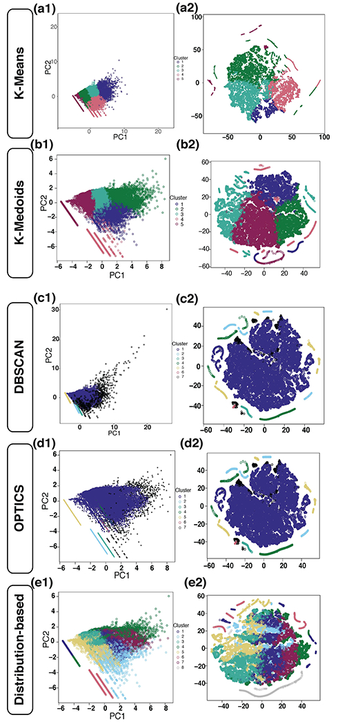
In the GFAP LPS object segmented from the hippocampus, multiple clustering methods were performed in order to elucidate the different ways objects inherently cluster. Using the silhouette method, k-means determined the optimal number of groups was k = 5. In order to see if these groups clustered similar ways using t-SNE, plots were created without including the cluster designation in the modeling dataframe. The PCA (a1) is color coordinated for the cluster assignments and a t-SNE plot (a2) shows that these objects have very little overlap other than where each cluster meets another. K-medoid shows similar performance to k-means and clusters generally do not overlap except for where one cluster is plotted next to the other (b1/b2). Next, DBSCAN determined the optimal number of clusters was 7 (minimum points = 30). Black objects are ones deemed noise and not included in any cluster nor do they create their own cluster. Predominately, objects fell into cluster 1 shown in indigo (c1/c2). Utilizing OPTICS, the optimal number of clusters was also 7 (minimum points = 30). Compared to the DBSCAN method, OPTICS only classified 2 objects differently in which they were moved from cluster 7 to the noise category (d1/d2). Although these clusters may form inherently through DBSCAN and OPTICS, they provide very little insight into the data due to the diversity of 20,511 objects classified into cluster 1. Distribution-based clustering was performed and determined the optimal number of clusters was 8. When plotting color-coded for the cluster designation, we can appreciate there are undefined cluster borders (e1/e2).

We then attempted to compare similar types of segmented objects between treatment class labels. To achieve this, vehicle-treated objects passed through the SVM prediction model to determine which type of LPS-treated object class the vehicle-treated object was most similar. This permitted us to evaluate the main morphological similarities and differences of gliosis in each region. To achieve this, we took each cluster and performed two supervised labeling workflows. First, we utilized a linear discriminate analysis (LDA) to predict treatment class label (vehicle or LPS) in each cluster designation, and the distribution of GFAP or ALDH1L1 objects are plotted in figures 9d and 10d. We note that in the hippocampus, GFAP clusters 1 and 3 show separation in their distribution along the LDA axis, and the main drivers of the separation are plotted as horizontal bar plots of the LDA coefficients (figure 9 e). Although hippocampal ALHD1L1 objects from cluster 1 showed near complete overlap on LDA (figure 10 d), random forest was still capable of having some significant predictive capacity. We conclude that in this cluster, non-linear relationships between variables underlies the differences in morphologies between the control and LPS-treated groups.

Utilizing linear discriminant analysis models, we found that some clusters showed more overlap in the density distribution compared to others (figures 9d and 10d). In addition, we found that the regional models created in figures 5 and 6 (a1–c1) generally had higher accuracy than the cluster specific models, likely reflecting an over-fitting phenomenon (figures 9f and 10f). From the LDA coefficients, we determined that biomarker texture is a principal feature that distinguishes treatment groups in the hippocampus in addition to fluorescent intensity (figure 9e and 10e).

In the neocortex, we found there was a variety of feature drivers that separated the vehicle and LPS objects from one another. For instance, shape features had higher importance for objects that were smaller (<0.5 μm). For larger objects, pixel texture and fluorescence intensity had higher coefficients relative to shape. We also found that a cluster of GFAP objects in the neocortex had overlap in morphology and the random forest models had poor accuracy at predicting reactivity state over the no information rate. These objects had low overlap in the LDA, but the random forest model had poor accuracy due to fewer objects for the models to train with. In the caudoputamen, the main distinction between vehicle and LPS objects was fluorescence intensity and Haralick features. Similar to the neocortex, the objects that were smaller in shape (generally < 0.5 μm) placed more importance on the shape features of the object to identify difference between the groups.

Discussion

In creating an automated image analysis workflow evaluating astroglial biomarkers in three different regions, we were able to unmask the subtle variations following systemic inflammation by implementing machine learning workflows. We found that the biomarkers GFAP and ALDH1L1 distinguish different objects and both can be utilized to evaluate reactive gliosis. We also determined that inflammation impacts astrocytes regionally and the variables determining reactivity state vary by region.

Importance of Biomarkers by Region

GFAP and ALDH1L1 both distinguish different objects. As seen in figure 3 (d1), a random forest model predicting the biomarker of segmented objects from vehicle-treated mice taken from the hippocampus was able to determine with 94.45% accuracy the biomarker the segmented object had been stained with. From this model, the main driver was the pixel intensity within the segmented object and how brightly it fluoresced (figure 3 e1). These data indicate different biomarkers highlight distinct cellular compartments as evidenced by their different shapes and textures. Inherently, the biomarkers label different parts of the astrocyte with GFAP labeling intermediate filaments that compose the cellular processes of particularly derived astrocytes, whereas ALDH1L1 more labels the cell body.

GFAP and ALDH1L1-labeled objects have unique morphologies within each neuroanatomical location studied. This conclusion is supported by our experiments where we generated a random forest with segmented objects of vehicle-treated mice which was capable of predicting neuroanatomical location (both GFAP and ALDH1L1 models had high accuracies determining location). In this model, pixel intensity had the highest importance (51%) when averaging the Gini Importance of each type of variable, whereas shape variables such as area and perimeter had the least importance on predicting neuroanatomical region (figure 3 e2–e3).

Lastly, GFAP and ALDH1L1 are both capable of predicting reactive gliosis. It is widely debated the ability of using GFAP to quantify gliosis (reviewed by (Liddelow & Barres, 2017; Liddelow et al., 2017). GFAP labels intermediate filaments while ALDH1L1 labels specific astrocytic proteins which are found in different regions within the astrocyte. We were able to determine that both biomarkers are capable of predicting gliosis with statistical significance (albeit it modest accuracy) when generating random forest models. However, these models are region-specific and poor predictors of gliosis in newly introduced regions. Therefore, in neuroanatomical assays quantifying gliosis using machine learning models, it is imperative that investigators incorporate region-specific controls in all comparisons. We also note that in generating supervised semantic segmentation workflows, such as WEKA or neural networks, a significant amount of training data from each anatomical region would be required.

Astrocytes undergo morphological region-specific changes during neuroinflammation

We utilized this well-studied experimental model to test the hypothesis that morphological changes in astrocytes in response to neuroinflammation represents a heterogenous, region-specific response. In addition to this, it was necessary to identify the importance of variables in a nonlinear approach. Models for each biomarker using PCA determined that shape features (area and perimeter) were more important in determining objects from vehicle-treated mice whereas pixel intensity (1^st percentile and mean fluorescence intensity) had higher importance for objects from LPS-treated mice within the hippocampus and neocortex. However, the caudoputamen models did not follow this trend. With the GFAP model, Haralick features had the highest importance for objects from both vehicle and LPS-treated mice. In the ALDH1L1 model, shape features were more important at identifying objects from LPS-treated mice whereas pixel intensity features were more important in objects from vehicle-treated mice. This further shows the importance of performing a regional approach to evaluating reactive gliosis due to some variables being high drivers of variation within different regions for each biomarker.

Through segmenting astrocytes into positively labeled objects, extracting morphological features, and evaluating them with nonlinear computational approaches, we show that it is possible to determine a difference in objects from vehicle-treated and LPS-treated mice. These findings elucidate that astrocytes undergo a heterogenous response to gliosis and the differences between regions and within clusters occurs based on nonlinear combination of multiple features. In summary, our data indicate that astrogliosis can be measured by both GFAP and ALDH1L1 immunofluorescent analysis, that astrogliosis results in heterogenous changes in these biomarkers that is region-specific, and that many of these changes cannot be measured using linear statistical models. Machine learning approaches permitted us to implement such non-linear analyses, thereby enabling us to discover the main morphological changes undergone during gliosis.

An additional approach to integrating machine learning into workflows would be the use of deep learning and utilizing neural networks to improve segmentation outcomes. More advanced 3-D reconstructive astrocyte image analyses techniques come at a computational cost, taking 25-30 minutes per image to complete (Kulkarni et al., 2015). In addition, this technique is successful in generating data for arborization quantification, it fails to include the entire astrocyte data for pixel segmentation. In recent years, astrocyte analysis has become more advanced using convolutional neural networks for counting the number of astrocytes and segmenting (Kayasandik, Ru, & Labate, 2020; Suleymanova et al., 2018). However, cell counting fails to elucidate the morphological changes astrocytes undergo following different disease states (Kayasandik et al., 2020). In addition, it is also time consuming for neuroanatomists to annotate ground truth images for segmenting training data. We suggest that using Otsu threshold, or other computationally basic segmentation methods depending on the type of cell being studied, as a bridging solution to time consuming manual ground truth segmentation. The deep learning astrocyte segmentation neural net developed by Kayasandik et al. had a high accuracy based on only 118 128x128 pixel images, however it is impractical to increase the training data set due to how time consuming it is to manually generate ground truth images (Kayasandik et al., 2020). We propose as a solution, it takes significantly less time to apply thresholding methods to automatically generate ground truths. A simple iterative cycle through multiple images would allow ground truths for full images containing multiple astrocytes rather than cropped 128 x 128 pixel single astrocyte images. We suggest combining basic segmentation methods for generating ground truth images, drastically increasing the training data that can be used with deep neural networks.

References

- Bergmeir C, & Benítez J (2012). Neural Networks in R Using the Stuttgart Neural Network Simulator: RSNNS. In (Vol. 46(7), pp. 1–26). Journal of Statistical Software.22837731 [Google Scholar]
- Bluemke DA, Moy L, Bredella MA, Ertl-Wagner BB, Fowler KJ, Goh VJ, … Weiss CR (2020). Assessing Radiology Research on Artificial Intelligence: A Brief Guide for Authors, Reviewers, and Readers-From the. Radiology, 294(3), 487–489. doi: 10.1148/radiol.2019192515 [DOI] [PubMed] [Google Scholar]
- Brynolfsson P, Nilsson D, Torheim T, Asklund T, Karlsson CT, Trygg J, … Garpebring A (2017). Haralick texture features from apparent diffusion coefficient (ADC) MRI images depend on imaging and pre-processing parameters. Sci Rep, 7(1), 4041. doi: 10.1038/s41598-017-04151-4 [DOI] [PMC free article] [PubMed] [Google Scholar]
- Cahoy JD, Emery B, Kaushal A, Foo LC, Zamanian JL, Christopherson KS, … Barres BA (2008). A transcriptome database for astrocytes, neurons, and oligodendrocytes: a new resource for understanding brain development and function. J Neurosci, 28(1), 264–278. doi: 10.1523/JNEUROSCI.4178-07.2008 [DOI] [PMC free article] [PubMed] [Google Scholar]
- Cao J, Wang JS, Ren XH, & Zang WD (2015). Spinal sample showing p-JNK and P38 associated with the pain signaling transduction of glial cell in neuropathic pain. Spinal Cord, 53(2), 92–97. doi: 10.1038/sc.2014.188 [DOI] [PubMed] [Google Scholar]
- Charrad M, Ghazzali N, Boiteau V, & Niknafs A (2014). NbClust: An R Package for Determining the Relevant Number of Clusters in a Data Set. In (Vol. 61, pp. 1–36). Journal of Statistical Software. [Google Scholar]
- Cortez P (2010). Data Mining with Neural Networks and Support Vector Machines Using the R/rminer Tool. In Lecture Notes in Artificial Intelligence 6171 (pp. 572–583). In Perner P (Ed.), Advances in Data Mining - Applications and Theoretical Aspects 10th Industrial Conference on Data Mining (ICDM 2010): Springer. [Google Scholar]
- Feilchenfeld Z, Yücel YH, & Gupta N (2008). Oxidative injury to blood vessels and glia of the pre-laminar optic nerve head in human glaucoma. Exp Eye Res, 87(5), 409–414. doi: 10.1016/j.exer.2008.07.011 [DOI] [PubMed] [Google Scholar]
- Franklin KBJ, & Paxinos G Paxinos and Franklin’s The mouse brain in stereotaxic coordinates (Fourth edition. ed.). [Google Scholar]
- Goceri E, Goksel B, Elder JB, Puduvalli VK, Otero JJ, & Gurcan MN (2017). Quantitative validation of anti-PTBP1 antibody for diagnostic neuropathology use: Image analysis approach. Int J Numer Method Biomed Eng, 33(11). doi: 10.1002/cnm.2862 [DOI] [PMC free article] [PubMed] [Google Scholar]
- Haralick RM, Shanmugam K, & Dinstein I (1973). Textural Features for Image Classification. Ieee Transactions on Systems Man and Cybernetics, Smc 3(6), 610–621. doi:Doi 10.1109/Tsmc.1973.4309314 [DOI] [Google Scholar]
- Javdani M, Ghorbani R, & Hashemnia M (2020). Histopathological Evaluation of Spinal Cord with Experimental Traumatic Injury Following Implantation of a Controlled Released Drug Delivery System of Chitosan Hydrogel Loaded with Selenium Nanoparticle. Biol Trace Elem Res. doi: 10.1007/s12011-020-02395-2 [DOI] [PubMed] [Google Scholar]
- Kassambara A, & Fabian M (2019). factoextra: Extract and Visualize the Results of Multivariate Data Analyses. In. [Google Scholar]
- Kayasandik CB, Ru W, & Labate D (2020). A multistep deep learning framework for the automated detection and segmentation of astrocytes in fluorescent images of brain tissue. Sci Rep, 10(1), 5137. doi: 10.1038/s41598-020-61953-9 [DOI] [PMC free article] [PubMed] [Google Scholar]
- Knijnenburg TA, Wessels LF, Reinders MJ, & Shmulevich I (2009). Fewer permutations, more accurate P-values. Bioinformatics, 25(12), i161–168. doi: 10.1093/bioinformatics/btp211 [DOI] [PMC free article] [PubMed] [Google Scholar]
- Krijthe J (2015). Rtsne: T-Distributed Stochastic Neighbor Embedding using a Barnes-Hut Implementation, . [Google Scholar]
- Kuhn M (2019). caret: Classification and Regression Training. In. [Google Scholar]
- Kulkarni PM, Barton E, Savelonas M, Padmanabhan R, Lu Y, Trett K, … Roysam B (2015). Quantitative 3-D analysis of GFAP labeled astrocytes from fluorescence confocal images. J Neurosci Methods, 246, 38–51. doi: 10.1016/j.jneumeth.2015.02.014 [DOI] [PubMed] [Google Scholar]
- Kursa MB, & Rudnicki WR (2010). Feature Selection with the Boruta Package. Journal of Statistical Software, 36(11), 1–13. [Google Scholar]
- Lee Y, Su M, Messing A, & Brenner M (2006). Astrocyte heterogeneity revealed by expression of a GFAP-LacZ transgene. Glia, 53(7), 677–687. doi: 10.1002/glia.20320 [DOI] [PubMed] [Google Scholar]
- Lein E, Borm LE, & Linnarsson S (2017). The promise of spatial transcriptomics for neuroscience in the era of molecular cell typing. Science, 358(6359), 64–69. doi: 10.1126/science.aan6827 [DOI] [PubMed] [Google Scholar]
- Liaw A, & Wiener M (2002). Classification and Regression by randomForest. R News, 2002(2), 18–22. [Google Scholar]
- Liddelow SA, & Barres BA (2017). Reactive Astrocytes: Production, Function, and Therapeutic Potential. Immunity, 46(6), 957–967. doi: 10.1016/j.immuni.2017.06.006 [DOI] [PubMed] [Google Scholar]
- Liddelow SA, Guttenplan KA, Clarke LE, Bennett FC, Bohlen CJ, Schirmer L, … Barres BA (2017). Neurotoxic reactive astrocytes are induced by activated microglia. Nature, 541(7638), 481–487. doi: 10.1038/nature21029 [DOI] [PMC free article] [PubMed] [Google Scholar]
- Luo Y, Xu NG, Yi W, & Du YX (2009). Effect of electroacupuncture on astrocytes in the marginal zone of cerebral ischemia locus in rats. Zhen Ci Yan Jiu, 34(2), 101–105. [PubMed] [Google Scholar]
- Maechler M, Rousseeuw P, Struyf A, Hubert M, & Hornik K (2019). cluster: Cluster Analysis Basics and Extensions. In (R package version 2.1.0. ed.). [Google Scholar]
- McKeever PE (1992). Computerized image analysis of distinct cell marker parameters of glial fibrillary acidic protein: intensity of immunofluorescence and topography in human glioma cultures. Cell Mol Biol, 38(2), 175–180. [PubMed] [Google Scholar]
- Meyer DM, Dimitriadou E, Hornik K, Weingessel A, & Leisch F (2019). e1071: Misc Functions of the Department of Statistics, Probability Theory Group (Formerly: E1071), TU Wien; In. [Google Scholar]
- Microsoft Corporation, & Weston S (2019). doParallel: Foreach Parallel Adaptor for the ‘parallel’ Package. In.
- Moffitt JR, Hao J, Bambah-Mukku D, Lu T, Dulac C, & Zhuang X (2016). High-performance multiplexed fluorescence in situ hybridization in culture and tissue with matrix imprinting and clearing. Proc Natl Acad Sci U S A, 113(50), 14456–14461. doi: 10.1073/pnas.1617699113 [DOI] [PMC free article] [PubMed] [Google Scholar]
- Nemzek JA, Hugunin KM, & Opp MR (2008). Modeling sepsis in the laboratory: merging sound science with animal well-being. Comp Med, 58(2), 120–128. [PMC free article] [PubMed] [Google Scholar]
- Neymeyer V, Tephly TR, & Miller MW (1997). Folate and io-formyltetrahydrofolate dehydrogenase (FDH) expression in the central nervous system of the mature rat. Brain Res, 766(1-2), 195–204. doi: 10.1016/s0006-8993(97)00528-3 [DOI] [PubMed] [Google Scholar]
- Norden DM, Trojanowski PJ, Villanueva E, Navarro E, & Godbout JP (2016). Sequential activation of microglia and astrocyte cytokine expression precedes increased Iba-1 or GFAP immunoreactivity following systemic immune challenge. Glia, 64(2), 300–316. doi: 10.1002/glia.22930 [DOI] [PMC free article] [PubMed] [Google Scholar]
- Oberheim NA, Goldman SA, & Nedergaard M (2012). Heterogeneity of astrocytic form and function. Methods Mol Biol, 814, 23–45. doi: 10.1007/978-1-61779-452-0_3 [DOI] [PMC free article] [PubMed] [Google Scholar]
- Oleś A, Pau G, Smith M, Sklyar O, & Huber W (2019). Package ‘EBImage’. 4.27.0. Retrieved from https://github.com/aoles/EBImage [Google Scholar]
- Pau G, Fuchs F, Sklyar O, Boutros M, & Huber W (2010). EBImage--an R package for image processing with applications to cellular phenotypes. Bioinformatics, 26(7), 979–981. doi: 10.1093/bioinformatics/btq046 [DOI] [PMC free article] [PubMed] [Google Scholar]
- Poostchi M, Silamut K, Maude RJ, Jaeger S, & Thoma G (2018). Image analysis and machine learning for detecting malaria. Transl Res, 194, 36–55. doi: 10.1016/j.trsl.2017.12.004 [DOI] [PMC free article] [PubMed] [Google Scholar]
- R Core Team. (2019). R: A Language and Environment for Statistical Computing. Vienna, Austria: R Foundation for Statistical Computing. [Google Scholar]
- Reemst K, Noctor SC, Lucassen PJ, & Hol EM (2016). The Indispensable Roles of Microglia and Astrocytes during Brain Development. Front Hum Neurosci, 10, 566. doi: 10.3389/fnhum.2016.00566 [DOI] [PMC free article] [PubMed] [Google Scholar]
- Roeder AH, Cunha A, Burl MC, & Meyerowitz EM (2012). A computational image analysis glossary for biologists. Development, 139(17), 3071–3080. doi: 10.1242/dev.076414 [DOI] [PubMed] [Google Scholar]
- Scrucca L, Fop M, Murphy T, & Raftery A (2016). mclust 5: clustering, classification and density estimation using Gaussian finite mixture models. In (Vol. 8, pp. 289–317). The R Journal. [PMC free article] [PubMed] [Google Scholar]
- Shah S, Lubeck E, Zhou W, & Cai L (2016). In Situ Transcription Profiling of Single Cells Reveals Spatial Organization of Cells in the Mouse Hippocampus. Neuron, 92(2), 342–357. doi: 10.1016/j.neuron.2016.10.001 [DOI] [PMC free article] [PubMed] [Google Scholar]
- Simko T. W. a. V. (2017). R package “corrplot”: Visualization of a Correlation Matrix (Version 0.84). [Google Scholar]
- Sofroniew MV, & Vinters HV (2010). Astrocytes: biology and pathology. Acta Neuropathol, 119(1), 7–35. doi: 10.1007/s00401-009-0619-8 [DOI] [PMC free article] [PubMed] [Google Scholar]
- Suleymanova I, Balassa T, Tripathi S, Molnar C, Saarma M, Sidorova Y, & Horvath P (2018). A deep convolutional neural network approach for astrocyte detection. Sci Rep, 8(1), 12878. doi: 10.1038/s41598-018-31284-x [DOI] [PMC free article] [PubMed] [Google Scholar]
- Venables WN, & Ripley BD (2002). Modern Applied Statistics with S (Vol. 4). New York: Springer. [Google Scholar]
- Vrbik I, Van Nest SJ, Meksiarun P, Loeppky J, Brolo A, Lum JJ, & Jirasek A (2019). Haralick texture feature analysis for quantifying radiation response heterogeneity in murine models observed using Raman spectroscopic mapping. PLoS One, 14(2), e0212225. doi: 10.1371/journal.pone.0212225 [DOI] [PMC free article] [PubMed] [Google Scholar]
- Wang X, Allen WE, Wright MA, Sylwestrak EL, Samusik N, Vesuna S, … Deisseroth K (2018). Three-dimensional intact-tissue sequencing of single-cell transcriptional states. Science, 361(6400). doi: 10.1126/science.aat5691 [DOI] [PMC free article] [PubMed] [Google Scholar]
- Wickham H (2016). ggplot2: Elegant Graphics for Data Analysis. New York: Springer. [Google Scholar]
- Yoon H, Walters G, Paulsen AR, & Scarisbrick IA (2017). Astrocyte heterogeneity across the brain and spinal cord occurs developmentally, in adulthood and in response to demyelination. PLoS One, 12(7), e0180697. doi: 10.1371/journal.pone.0180697 [DOI] [PMC free article] [PubMed] [Google Scholar]
- Zilles K, Hajós F, Kálmán M, & Schleicher A (1991). Mapping of glial fibrillary acidic protein-immunoreactivity in the rat forebrain and mesencephalon by computerized image analysis. J Comp Neurol, 308(3), 340–355. doi: 10.1002/cne.903080303 [DOI] [PubMed] [Google Scholar]
Associated Data
This section collects any data citations, data availability statements, or supplementary materials included in this article.