On the Design and the Analysis of Stratified Biomarker Trials in the Presence of Measurement Error

Abstract

A major emphasis in precision medicine is to optimally treat subgroups of patients who may benefit from certain therapeutic agents. And as such, enormous resources and innovative clinical trials designs in oncology are devoted to identifying predictive biomarkers. Predictive biomarkers are ones that will identify patients that are more likely to respond to specific therapies and they are usually discovered through retrospective analysis from large randomized phase II or phase III trials. One important design to consider is the stratified biomarker design, where patients will have their specimens obtained at baseline and the biomarker status will be assessed prior to random assignment. Regardless of their biomarker status patients will be randomized to either an experimental arm or the standard of care arm. The stratified biomarker design can be used to test for a treatment-biomarker interaction in predicting a time-to event outcome. Many biomarkers, however, are derived from tissues from patients, and hence their levels may be heterogeneous. As a result, biomarker levels may be measured with error and this would have an adverse impact on the power of a stratified biomarker clinical trial. We present a trial design and an analysis framework for the stratified biomarker design. We show that the naïve test is biased and provide bias-corrected estimators for computing the sample size and the 95% confidence interval when testing for a treatment-biomarker interaction. We propose a sample size formula that adjusts for misclassification and apply it in the design of a phase III clinical trial in renal cancer.

1 |. INTRODUCTION

A major emphasis in precision medicine is to optimally treat subgroups of patients who may benefit from certain therapeutic agents^1,2,3. And as such, enormous resources and innovative clinical trials in oncology are devoted to identifying predictive biomarkers^4,5,6,7. Predictive biomarkers are ones that will identify patients that are most likely to respond to specific therapies and they are usually discovered through retrospective analysis from either large randomized phase II or phase III trials^3,8. A statistical test for the biomarker-treatment interaction is often performed to determine whether a biomarker is predictive of the outcome for the treatment under study.

If properly designed, biomarker driven trials hold the promise of discovering subgroups of patients that would benefit the most from experimental therapies^6,9. One important design to consider is the stratified biomarker design where patients have their specimens obtained at baseline and the biomarker status will be assessed prior to random assignment. Regardless of their biomarker status, patients will be randomized to either an experimental arm or the standard of care arm⁹. In other words, the biomarker status (positive or negative) for all patients must be known prior to their randomization (Figure 1).

FIGURE 1.

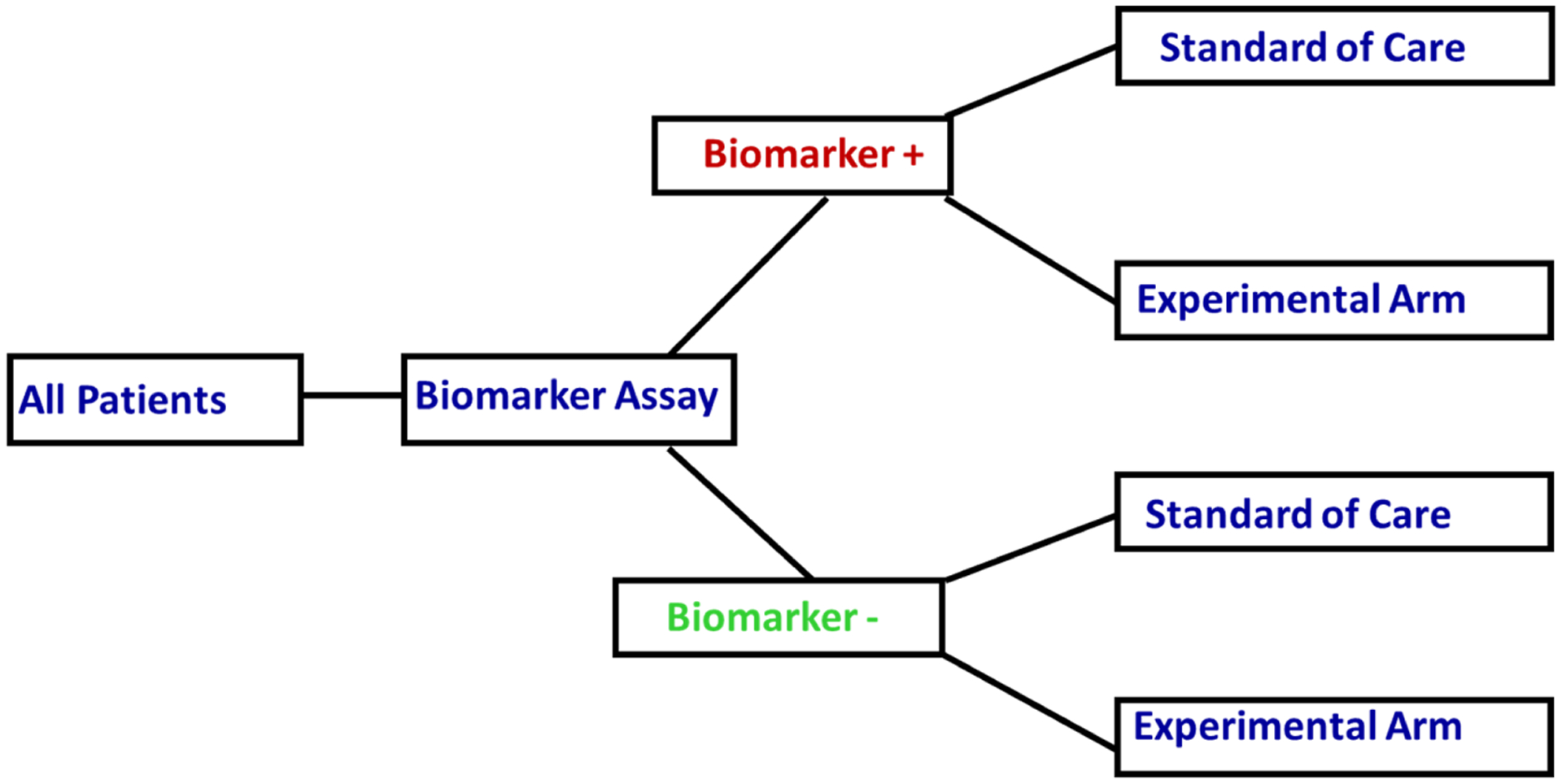
A Stratified Biomarker Design

Thus, one of the primary objectives of the stratified biomarker design is to prospectively test whether an experimental agent will improve clinical outcomes in subgroups of patients based on their biomarker status. When there is insufficient level of evidence if the biomarker is predictive of outcome, the stratified biomarker design may be an appropriate approach in answering the primary question for testing whether the biomarker is predictive of the outcome⁹. Specifically, the stratified biomarker design can be used to test for treatment-biomarker interaction in a clinical trial¹⁰. Other primary interests of a stratified biomarker design are to investigate the effect of the treatment on the outcome within the same biomarker status or to test if the clinical outcomes within the same treatment are different by the biomarker status.

We provide two examples of clinical trials that were designed as the stratified biomarker trials^11,12. The first example is the MARVEL trial where patients with second line advanced non–small cell lung cancer were randomly assigned to either erlotinib or pemetrexed with randomization stratified by epidermal growth factor receptor gene (EGFR) status as measured by fluorescent in situ hybridization (FISH)¹¹. Another example is the Tarceva Italian Lung Optimization (TAILOR) trial was designed as a hybrid stratified biomarker design, where EGFR negative mutation patients were randomly assigned to the erlotinib or docetaxel arms, stratified by the negativity mutation for EGFR 19 or 21¹². The design of the TAILOR trial was revised based on the recommendation from the data and safety monitoring committee¹³

In cancer, several biomarkers are derived from tissues of the patients. The levels of the biomarkers are known to be heterogeneous within the tissue. Examples of tissue biomarkers are EFGR levels (lung cancer)¹⁴, human epidermal growth factor receptor 2 (HER2; breast cancer)¹⁵, retinoblastoma (prostate cancer)¹⁶, and hepatocyte growth factor (HGF; renal cancer)¹⁷. Often there are several assays available for testing a single biomaker and different assays would yield different sensitivity and specificity. The quality of specimens play an important role on the sensitivity and specificity as lower specimens would tend to have decreased sensitivity and specificity¹⁸. As an example, we consider HER2 where several assays are approved for clinical testing to determine the HER2 status for a breast cancer patient. These assays include immunohistochemistry, FISH, silver in situ hybridization and chromogenic in situ hybridization¹⁹. However, it has been estimated that about about 20% of HER2 specimens might result in an incorrect test results¹⁹. In a study comparing different assays for HER2 testing for breast cancer, the sensitivity ranged from 0.961 to 1, whereas the specificity of ranged from 0.74 to 0.98¹⁸.

We are interested in designing a phase III clinical trial in patients with metastatic renal cancer. We consider a two arm trial: experimental treatment versus standard of care, with Z as the treatment indicator, where Z = 1 if experimental treatment and Z = 0 for the standard of care. The biomarker is KI-67 and we assume that it is dichotomous and is denoted by G (=1 if positive or =0 if negative).

In the present article, we investigate the adverse effects of biomarker misclassification on the design and analysis of a stratified biomarker clinical trial when the primary outcome is a time-to-event endpoint that is subject to censoring. We show that the misclassification error has profound adverse effects on the power of the test, required sample size, accrual period and the total duration of the trial. We propose methods to adjust for the classification error in the biomarker status for both the design and analysis stages.

The remainder of this article is organized as follows. In Section 2.1, we introduce notations and preliminary results concerning the design of a stratified biomarker trial in the presence of classification error. We make a distinction in correcting for the measurement error whether it is at the design or the analysis stage. In Section 2.2, we present the naïve estimator in the presence of measurement error and we describe the bias corrected (BC) and the adaptive BC estimator for the naïve estimators in Section 2.3. In Section 2.4 we provide a sample size computation and in Section 2.5 we demonstrate the adverse effects of misclassification error on trial duration and adjust for trial duration. The effect of misclassification on the analysis stage is discussed in Section 3. We present the concept of the SIMulation-EXtrapolation approach. We perform simulation studies in Section 4, and examine the performance of the different estimators in Section 4.1. We then apply our sample size to a phase III renal cancer trial in Section 4.2. Lastly, we discuss the findings in Section 5.

2 |. DESIGN PHASE

2.1 |. Preliminary

Consider a two-arm randomized trial where treatment assignment Z = 0, 1 indicates control and experimental arms, respectively; and a binary biomarker with status G = 0, 1 indicates the absence and presence of the biomarker. Assuming the survival time of the treatment group z and biomarker status g has an exponential distribution with mean θ_gz (or hazard rate λ_gz = 1/θ_gz), following the convention of Peterson and George²⁰, we define the primary interest, the treatment-by-biomarker interaction as γ = θ₀₁θ₁₀/θ₀₀θ₁₁.

In a randomized clinical trial, patients’ survival times are subject to censoring due to various reasons, such as the patient does not experience the event of interest during the trial, or the patient experiences an adverse events, etc. Let t_i and δ_i be the observed survival time and censoring indicator, respectively, for the ith patient, and Γ_gz = {i : g_i = g,_i = z} be the collection of indices of patients randomized to treatment z with biomarker g. Under the exponential assumption, θ_gz can be estimated using the maximum likelihood estimator (MLE). The MLE has an analytical form ${\widehat{\theta }}_{gz}={\sum }_{i\in {\Gamma }_{gz}}{t}_i/{\sum }_{i\in {\Gamma }_{gz}}{\delta }_i$ whose asymptotic distribution is given by ${\widehat{\theta }}_{gz}~AN\left({\theta }_{gz},{\theta }_{gz}^2/{\sum }_{i\in {\Gamma }_{gz}}{\delta }_i\right)$. In addition, the minus logarithm of the $\text{MLE}-\text{log}\left({\widehat{\theta }}_{gz}\right)$, also the logarithm of the MLE of the hazard rate, is asymptotically normal $-\text{log}\left({\widehat{\theta }}_{gz}\right)~N\left(-\text{log}\left({\theta }_{gz}\right),1/{\sum }_{i\in {\Gamma }_{gz}}{\delta }_i\right)$ per the delta method. The MLE of the treatment-biomarker interaction can be constructed accordingly, say $\widehat{\gamma }={\widehat{\theta }}_{01}{\widehat{\theta }}_{10}/{\widehat{\theta }}_{00}{\widehat{\theta }}_{11}$. It follows that the asymptotic distribution of the logarithm of the MLE of γ has a simple form

$$\text{log}(\widehat{\gamma })~N\left(\text{log}(\gamma ),\sum _{g=0}^1\sum _{z=0}^1\frac{1}{{\sum }_{i\in {\Gamma }_{gz}}{\delta }_i}\right)$$ (1)

Assuming equal number of events per stratum (only under H₀),²⁰ derived a sample size for a two-sided size α test H₀ : log(γ) = 0. At power 1 − β, the common sample size is

$$\left|{\Gamma }_{gz}\right|\ge \frac{4{\left({\Phi }^{-1}(1-\alpha /2)+{\Phi }^{-1}(1-\beta )\right)}^2}{{(\text{log}(\gamma ))}^2},$$ (2)

where Φ(·) is the cumulative standard normal distribution.

2.2 |. Measurement Error

When the biomarker G is observed with error, or subject to misclassification, which is not unusual in many biomarker assays^21,22,23,18, the accuracy of the observed marker status M can be evaluated utilizing the most commonly used measures:

• Sensitivity: π_sens = P(M = 1|G = 1),

• Specificity: π_spec = P(M = 0|G = 0),

• Positive predictive values: π_pp = P(G = 1|M = 1), and

• Negative predictive values: π_np = (G = 0|M = 0).

M is the observed prevalence and is often estimated from datasets whereas G is the prevalence of the biomarker from the true population. Furthermore, we denote the prevalence (G = 1) = π_G and P(M = 1) = π_M. Throughout this article, we assume π_G, π_sens and π_spec are known and π_sens + π_spec > 1 which should hold for any reliable assay. With the knowledge of these three values, the observed marker prevalence, positive and negative predictive values can be easily derived.

In the presence of measurement error, we denote a naïve estimators of ${\theta }_{gz}={\tilde{\theta }}_{gz}^N={\sum }_{i\in {\tilde{\Gamma }}_{gz}}{t}_i/{\sum }_{i\in {\tilde{\Gamma }}_{gz}}{\delta }_i$, where ${\tilde{\Gamma }}_{gz}=\left\{i:m_i=g,z_i=z\right\}$. The asymptotic properties of the naïve estimators can be established analogously

$${\tilde{\theta }}_{gz}^N~N\left({\vartheta }_{gz},\frac{{\vartheta }_{gz}^2}{{\sum }_{i\in {\tilde{\Gamma }}_{gz}}{\delta }_i}\right),$$ (3)

where the ϑ_gz = E(T|M = g,Z = z) which can be written as a linear combination of θ_gz

$${\vartheta }_{gz}=\sum _{g^{\prime }=0}^{1}E\left(T\mid G=g^{\prime },Z=z\right)P\left(G=g^{\prime }\mid M=g\right)=\sum _{g^{\prime }=0}^1{\theta }_{g^{\prime }z}P\left(G=g^{\prime }\mid M=g\right).$$ (4)

It is evident from equation (4), that the naïve estimator is not a consistent estimator unless π_pp = π_np = 1 or θ_0z = θ_1z for z ∈ {0, 1}. Another special case is that, if the true interaction γ = 1, the naïve interaction estimators ${\tilde{\gamma }}^N={\tilde{\theta }}_{10}{\tilde{\theta }}_{01}/{\tilde{\theta }}_{00}{\tilde{\theta }}_{11}$ is still asymptomatically unbiased, even though the estimator of individual θ_gz is biased.

2.3 |. Asymptotically Unbiased Estimators

While the identity in (4) indicates that the naïve estimator is asymptotically biased, it sheds light on how to correct for the bias and for deriving an asymptotically unbiased estimator. We denote ${\tilde{\theta }}^{BC}$ as a bias-corrected (BC) estimator which, by the principle of the method of moments, can be found by solving the linear system plugging g = {0, 1} and z = {0, 1} into (4), namely

$$\left[\begin{array}{cccc}{\pi }_{np}& 0& 1-{\pi }_{np}& 0\\ 0& {\pi }_{np}& 0& 1-{\pi }_{np}\\ 1-{\pi }_{pp}& 0& {\pi }_{pp}& 0\\ 0& 1-{\pi }_{pp}& 0& {\pi }_{pp}\end{array}\right]\left[\begin{array}{l}{\tilde{\theta }}_{00}^{BC}\hfill \\ {\tilde{\theta }}_{01}^{BC}\hfill \\ {\tilde{\theta }}_{10}^{BC}\hfill \\ {\tilde{\theta }}_{11}^{BC}\hfill \end{array}\right]=\left[\begin{array}{c}{\tilde{\theta }}_{00}^N\\ {\tilde{\theta }}_{01}^N\\ {\tilde{\theta }}_{10}^N\\ {\tilde{\theta }}_{11}^N\end{array}\right]$$ (5)

As the solution to the linear system $A{\tilde{\theta }}^{BC}={\tilde{\theta }}^N$, the BC estimator can be expressed as a linear combination of the naïve estimator in the form ${\tilde{\theta }}^{BC}=A^{-1}{\tilde{\theta }}^N$, where the inverse matrix of A can be explicitly written as

$${\mathit{A}}^{-1}=\frac{1}{\left({\pi }_{pp}+{\pi }_{np}-1\right)}\left[\begin{array}{cccc}{\pi }_{pp}& 0& -\left(1-{\pi }_{np}\right)& 0\\ 0& {\pi }_{pp}& 0& -\left(1-{\pi }_{np}\right)\\ -\left(1-{\pi }_{pp}\right)& 0& {\pi }_{np}& 0\\ 0& -\left(1-{\pi }_{pp}\right)& 0& {\pi }_{np}\end{array}\right].$$ (6)

Moreover, since the BC estimator is a linear transformation of the naïve estimator, its asymptotic distribution has a simple form ${\tilde{\theta }}^{BC}~AN\left(\theta ,A^{-1}\text{cov}\left({\tilde{\theta }}^N\right)A^{-T}\right)$, where the covariance matrix $\text{cov}\left({\tilde{\theta }}^N\right)$ is a diagonal matrix with variances of each naïve estimator ${\tilde{\theta }}_{gz}^N$ on the diagonal. The covariance structure suggests that the BC estimator is more efficient than the naïve estimator as long as π_pp < 1 and π_np < 1.

Upon correcting the bias of the naïve estimator, we propose to estimate the interaction using the BC estimator and denote the interaction estimator as ${\tilde{\gamma }}^{BC}=\frac{{\theta }_{01}^{BC}{\theta }_{10}^{BC}}{{\tilde{\theta }}_{00}^{BC}{\tilde{\theta }}_{11}^{BC}}$. Let $h(\theta )=\text{log}\frac{{\theta }_{01}{\theta }_{10}}{{\theta }_{00}{\theta }_{11}}$, then by continuity $h\left({\tilde{\theta }}^{BC}\right)\stackrel{p}{\to }\text{log}\gamma$ and by the delta method $\text{var}\left(h\left({\tilde{\theta }}^{BC}\right)\right)={\nabla }_{\theta }^T{A}^{-1}\text{Cov}\left({\tilde{\theta }}^N\right)A^{-T}{\nabla }_{\theta }$, where ▽_θ is a 4×1 gradient vector of h with respect to each θ_gz. By carrying out the matrix multiplication, the variance can be written specifically

$${\left({\pi }_{pp}+{\pi }_{np}-1\right)}^{-2}\left\{\frac{1}{\left|{\Gamma }_{00}\right|}\frac{{\vartheta }_{00}^2{\vartheta }_{10}^2}{{\theta }_{00}^2{\theta }_{10}^2}+\frac{1}{\left|{\Gamma }_{01}\right|}\frac{{\vartheta }_{01}^2{\vartheta }_{11}^2}{{\theta }_{01}^2{\theta }_{11}^2}+\frac{1}{\left|{\Gamma }_{10}\right|}\frac{{\vartheta }_{00}^2{\vartheta }_{10}^2}{{\theta }_{00}^2{\theta }_{10}^2}+\frac{1}{\left|{\Gamma }_{11}\right|}\frac{{\vartheta }_{01}^2{\vartheta }_{11}^2}{{\theta }_{01}^2{\theta }_{11}^2}\right\}$$ (7)

We conclude this section by making some important observations regarding the BC estimator and its limitations. First, the BC estimator exists if the A matrix is invertible, i.e. π_pp +π_np ≠ 1. This condition holds for any reliable assay under our assumption π_sens +π_spec > 1. However, just because a solution exists does not mean that it is a valid estimate, since a negative estimate could be produced under some circumstances. Take ${\tilde{\theta }}_{00}^{BC}$ as an example, the estimate could be negative if ${\pi }_{pp}{\tilde{\theta }}_{00}^N\le \left(1-{\pi }_{np}\right){\tilde{\theta }}_{10}^N$, for some small positive predictive value or much larger ${\tilde{\theta }}_{10}^N$ estimate.

Second, when designing a new clinical trial, prior knowledge regarding the true prevalence π_G is required in order that the positive and negative predictive values can be calculated accordingly. Conversely, upon trial completion, we can first estimate the observed prevalence by the sample prevalence, and then solve the true prevalence backwards using the identity

$${\widehat{\pi }}_G=\frac{\widehat{\mathit{P}}(\mathit{M}=1)+{\pi }_{\mathit{\text{spec}}}-1}{{\pi }_{\text{sens }}+{\pi }_{\mathit{\text{spec}}}-1},$$ (8)

where $\widehat{\mathit{P}}(\mathit{M}=1)=\left(\left|{\tilde{\Gamma }}_{10}\right|+\left|{\tilde{\Gamma }}_{11}\right|\right)/N$ is the sample prevalence, and N is the total number of patients. We refer to the BC estimator that is plugged in the estimated π_G, π_ppv and π_npv as the adaptive BC estimator in the simulation section.

Third, the BC estimator suffers from another limitation in some cases where the estimand is not individual θ_gz, but rather a linear combination of them. As an example, take the hypothesis H₀ : k^Tθ = 0, where k is a 4×1 vector. If k satisfies the condition

$$A^{-T}k=ck,$$ (9)

where c is some positive constant, then the test statistic based on the BC estimator will degenerate to that based on the naïve estimator, therefore nullifying the bias-correction property. A close examination of equation (9) suggests k is an eigenvector or a linear combination of the eigenvectors of A^−T. Given A⁻¹ has a simple form given in (6), some algebra shows that the four unique eigenvectors of A^−T are given by

$$\left[\begin{array}{cccc}1& 0& 1-{\pi }_{pp}& 0\\ 0& 1& 0& 1-{\pi }_{pp}\\ -1& 0& 1-{\pi }_{np}& 0\\ 0& -1& 0& 1-{\pi }_{np}\end{array}\right].$$ (10)

Some commonly-used contrasts, such as the treatment effect, k^T = (−0.5 0.5 − 0.5 0.5), and the marker effect, k = (−0.5 − 0.5 0.5 0.5), are linear combinations of the first two eigenvectors. As a result, the corrected test statistic is not an ideal procedure to test if any of this type of effect is zero.

Lastly, we build up the BC estimator that is based on the exponential distribution yet the linear system shown in (5) can be applied to any valid (non)parametric mean estimator. For instance, the naïve estimator can be replaced with the area under the Kaplan-Meier survival curve. However, this replacement is ideally geared toward numerical calculation as the theoretical properties of the BC estimator becomes prohibitively challenging to derive. We will demonstrate the validity of such replacement through numerical examples in Section 4.

2.4 |. Sample Size and Trial Duration

We illustrated the adverse effects of the measurement error and proposed a bias-corrected estimator in the previous section when the biomarker is subject to measurement error. When designing a clinical trial using a time-to-event end-point, a two-stage approach is used where in the first stage the required number of events is computed. In the second stage, the required number of patients is calculated as a function of enrollment rate per unit of time (months), hypothesized hazard ratio, length of enrollment period, follow-up period and the hazard rates for patients randomized to the experimental and standard of care arms. This approach has been thoroughly investigated in Peterson and George^20,24, and Rubinstein²⁵. We present the trial duration estimate in this section. In this framework, we denote the enrollment rate from each stratum as e_gz, the enrollment period as $\mathcal{T}$, and the follow-up period as $\mathcal{F}$. To simplify exposition, the randomization ratio is compounded with the overall accrual rate. From^20,25, the relationship between the sample size and the enrollment period is given by

$$E\left(\left|{\Gamma }_{gz}\right|\right)=e_{gz}{\theta }_{gz}\left[{\theta }_{gz}^{-1}\mathcal{T}-e^{-{\theta }_{gz}^{-1}F}\left(1-\text{exp}\left(-{\theta }_{gz}^{-1}\mathcal{T}\right)\right)\right]$$ (11)

Equation (11) will then be plugged into the variance of h(θ^BC) given in Equation (7) by replacing the number of event |Γ_gz| with a function of θ_gz, e_gz, $\mathcal{F}$ and $\mathcal{T}$. However, the variance becomes very complicated and makes analytical derivation prohibitively challenging. We implement the variance calculation and subsequent power calculation in R 3.5.0, and illustrate the results in the following section. The program is available on-line (https://susanhalabi.shinyapps.io/survival_interaction/).

2.5 |. Adjustment of Trial Duration

We demonstrate the adverse impact of measurement error on the power and enrollment duration in this section. For illustrative purposes, we set the mean survival time at θ^T = (8,8,10,25)∕log2 (or equivalently medians survival times of 8, 8, 10, and 25 months), marker prevalence π_G = 0.3, follow-up period of 36 months, and assume an overall enrollment rate of 20 patients per month and a two-sided type I error of 0.05. Patients will be randomized in a 1:1 ratio to the standard of care and experimental arms stratified by the biomarker status. In the first illustration, we vary the enrollment period from 12 to 36 months and present the power for different combinations of sensitivity and specificity (Figure 2). Superimposed on Figure 2 are contour curves showing the combinations of sensitivity and specificity levels where a trial is powered at 70% to 90%.

FIGURE 2.

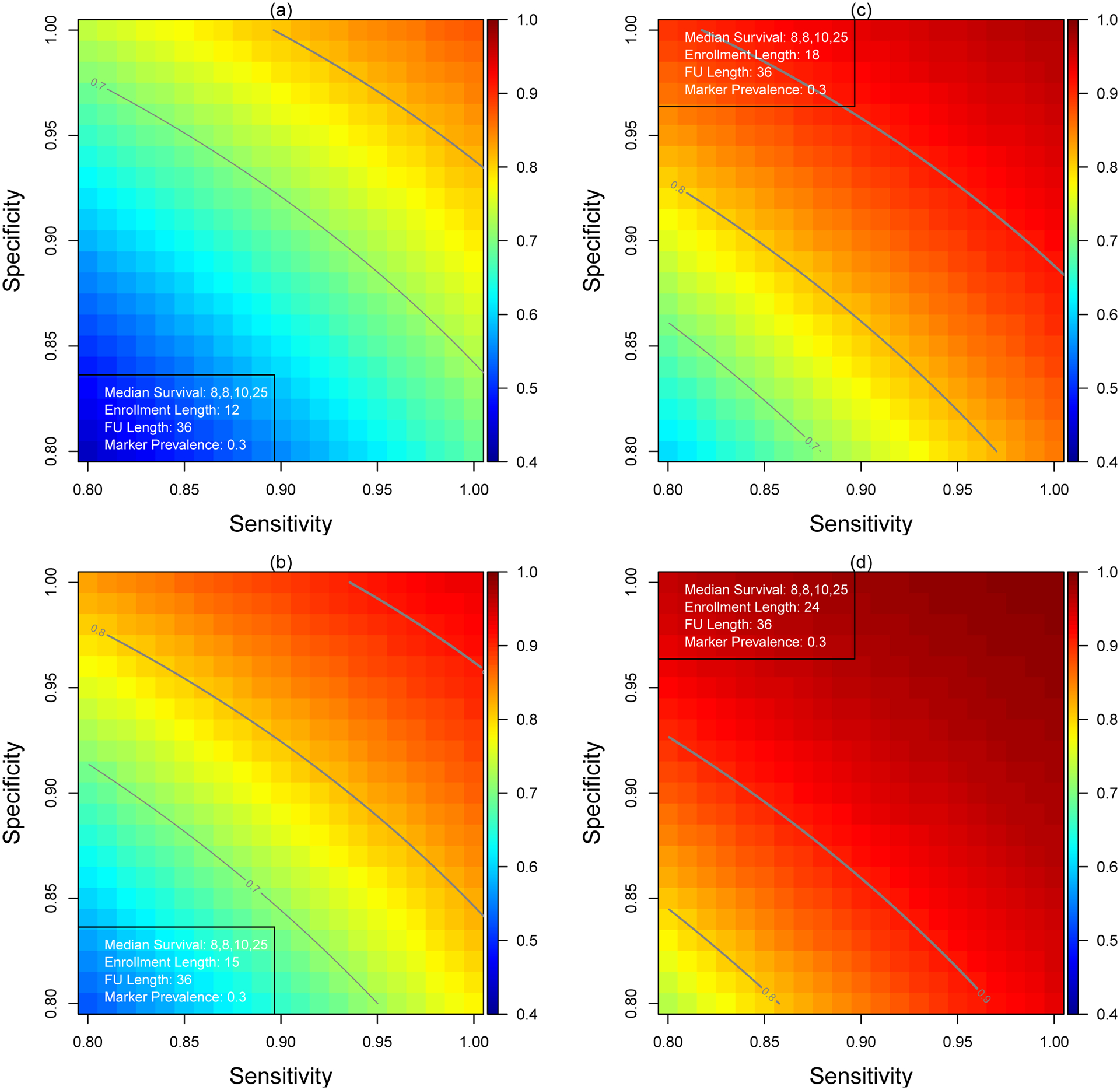
Statistical Power for Various Combinations of Sensitivity and Specificity

When the length of the enrollment period and follow-up period are 12 and 36 months (panel(a)), respectively, the study is adequately powered at 0.872 to test the interaction (log(2) = 0.693) if the biomarker is not subjected to measurement error (π_sens = π_spec = 1). The power decreases rapidly to 0.789 and 0.684 even with adequate sensitivity and specificity, π_sens = π_spec = 0.95 and π_sens = π_spec = 0.90, respectively.

In the second illustration, we fix the power at 0.75, 0.80, 0.85 and 0.90 and solve backward the minimal length of enrollment period to achieve the required power across a range of sensitivity and specificity. The results are presented in Figure 3. Without measurement error, it takes 13.1 months to enroll sufficient patients to test the interaction at 90% power (panel (d)). The trial length increases from 16.4 months to 20.8 months when π_sens = π_spec = 0.95 and π_sens = π_spec = 0.90, respectively.

FIGURE 3.

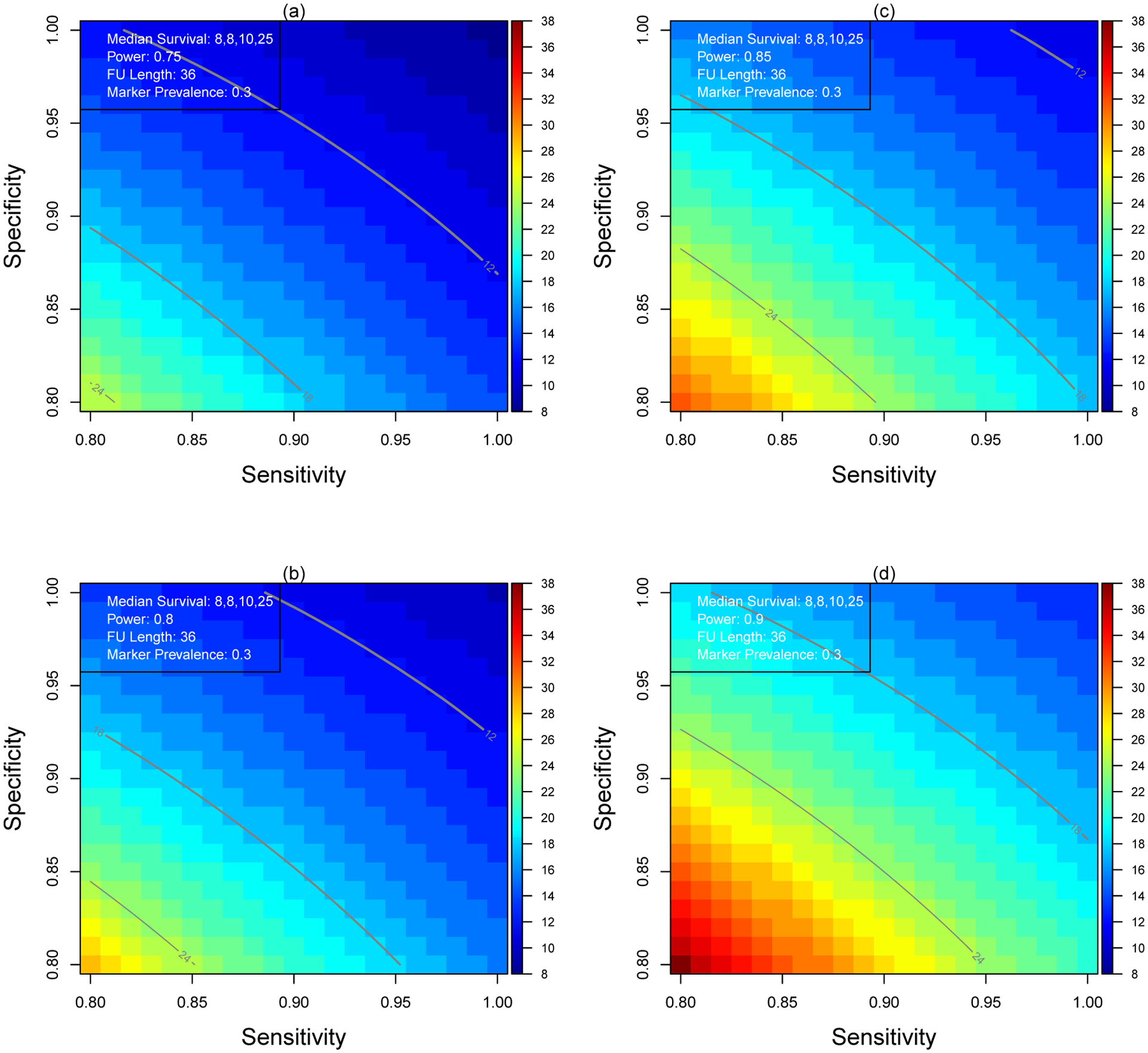
Minimum Enrollment Length for Various Combinations of Sensitivity and Specificity

3 |. ANALYSIS PHASE

In the previous sections, we demonstrated how the measurement error in the biomarker could negatively impact the estimation procedure and subsequently undermine the power of the study. Additionally, a bias-corrected estimation procedure was proposed and a sufficiently-powered sample size calculation is recommended. In this section, we focus on the analysis phase once a trial reaches a key milestone (number of events) and the data are mature for the final analysis.

3.1 |. SIMulation-EXtrapolation Approach

A well-powered clinical trial with a sample size can be calculated by leveraging the theoretical property of the BC estimator. However, the BC estimator does not guarantee positivity of the estimate and thus would limit its application. In the measurement error literature, a generic bias correction procedure has been proposed via a computational method. In particular, we propose to leverage the SIMulation-EXtrapolation (SIMEX) approach to correct for the measurement error and derive an unbiased estimate. The SIMEX approach has been extensively studied in various linear regression context. The reader is referred to the monograph by Carroll²⁶ for a comprehensive review. More recently, Küchenhoff²⁷ expanded the application to a case where a binary response or predictor is observed with error. Building on the MC-SIMEX method²⁷, we outline a novel extension to resolve the challenges in analyzing a stratified biomarker study in the presence of measurement error.

Following the notations used in the previous section, we characterize relationship between the observed and the true biomarker through the transition matrix

$$\Pi =\left[\begin{array}{cc}{\pi }_{\text{spec }}& 1-{\pi }_{\text{sens }}\\ 1-{\pi }_{\text{spec }}& {\pi }_{\text{sens }}\end{array}\right],$$ (12)

and define a power transformation of the transition matrix

$${\Pi }^v=E{\Lambda }^v{E}^{-1},$$

where Λ is a diagonal matrix of the eigenvalues of Π, and E is the corresponding matrix of eigenvectors. The transition matrix Π defines the misclassification process from the true biomarker G to the observed biomarker M. Similarly, we can use the power-transformed transition matrix Π^υ to define another misclassified version of M, say M*. If the two misclassification processes are independent, then M* is related to the true biomarker G by the transition matrix Π^1+υ. We later use the notation M_i* = MC[Π^υ](M_i) to describe the relationship between M_i and $M_i^{*}$.

We follow the traditional MC-SIMEX procedures outlined in^27,28 and propose a two-step procedure to estimate the parameter of interest, treatment-biomarker interaction.

Simulation Step:

Using a fixed grid points of 0 < υ₁ < … < υ_K, simulate B pseudo biomarker status for each patient

$$m_{b,i}^{*}=\mathit{M}\mathit{C}\left[{\Pi }^{v_k}\right]\left(m_i\right),i=1,\dots ,\sum _{g,z}\left|{\tilde{\Gamma }}_{gz}\right|;k=1,\dots ,\mathit{K};b=1,\dots ,\mathit{B}.$$ (13)

For each simulated data, we estimate the interaction using the naïve approach as if there is no misclassification, and then take the average as the final estimate at the grid point υ_k

$$\check{\gamma }\left(v_k\right)={\mathit{B}}^{-1}\sum _{b=1}^{\mathit{B}}{\tilde{\gamma }}^N\left(t_i,{\delta }_i,m_{b,i}^{*},z_i\right),k=1,\dots ,\mathit{K}.$$ (14)

Extrapolation Step:

We model the relationship between (1+υ) and $\check{\gamma }$ using a linear regression model, say $\check{\gamma }=g(1+v)$, where g(·) is a polynomial function with certain unknown parameters that can be estimated by the least squares approach using the data pair ${\left[1+v_k,\check{\gamma }\left(v_k\right)\right]}_{k=1}^K$. The final MC-SIMEX estimator is then given by extrapolating the function at 0, that is ${\check{\gamma }}^{\mathit{\text{SIMEX}}}=\check{g}(0)$, which corresponds to υ = −1.

The success of the MC-SIMEX estimator depends on the correct specification of (·), which is unknown in practice. Polynomial function is a popular alternative and provides a good approximation^27,29,30. We implement a cubic function for g in this article.

In addition to a point estimate, the MC-SIMEX algorithm also provides a variance estimate without the computational burden. At a given grid point υ_k, we calculate two sources of variability, V_sim and V_naive, defined respectively as

$$V_{sim}\left(v_k\right)={\mathit{B}}^{-1}\sum _{b=1}^{\mathit{B}}{\left[{\tilde{\gamma }}^N\left(t_i,{\delta }_i,m_{b,i}^{*},z_i\right)-\check{\gamma }\left(v_k\right)\right]}^2,k=1,\dots ,\mathit{K},$$

$$V_{\mathit{\text{naive }}}\left(v_k\right)={\mathit{B}}^{-1}\sum _{b=1}^{\mathit{B}}\text{var}\left({\tilde{\gamma }}^N\left(t_i,{\delta }_i,m_{b,i}^{*},z_i\right)\right),k=1,\dots ,\mathit{K}.$$

Stefanski³⁰ showed that the variance estimate for the SIMEX estimator is given by extrapolating the difference V_naive(υ) – V_sim(υ) at υ = −1. For this purpose, another cubic regression model is built to characterize the relationship between (1 + υ_k) and V_naive(υ_k) – V_sim(υ_k).

4 |. SIMULATIONS STUDY

We demonstrate the efficiency of the proposed BC and the SIMEX estimators in the analysis phase using simulations in this section. The simulation settings are similar to those described and utilized in Sections 2.4 and 2.5. We assume a total of 500 and 1000 patients will be enrolled and their true biomarker status and treatment group are random samples from Bernoulli distributions with prevalence rate π_G = 0.3 and patients are randomized to the standard of care and the experimental arms in a 1:1 allocation ratio. The biomarker sensitivity and specificity are set at two levels: 0.90 and 0.85. Conditional on the biomarker status and treatment assignment, the survival times are generated from two scenarios. In the first setting, the survival times are generated from exponential distributions with means θ^T = (θ₀₀,15,16,30) (or this corresponds to medians survival times (months): M₀₀, 10.4, 11.9, 20.8) and the censoring time follows an independent exponential distribution with mean 20. The mean survival time θ₀₀ is chosen such that the interaction ranges from 1 to 2. By setting the θ_gz’s at this level, the censoring rate in group G = 0, Z = 1 ranges from 17% (θ₀₀ = 8) to 29%(θ₀₀ = 4), and the censoring rates in the remainder three groups are 43%, 44%, and 60%, respectively. In the second scenario, we generate the survival times from the Weibull distribution with shape parameters 1,1.5,1.75 and 2. The scale parameters are chosen such that the mean survival time from the Weibull distribution equals the mean exponential survival time used in the first scenario. Note that in the first scenario we used the MLE to estimate the unknown parameter θ; whereas in the second scenario the mean survival time is estimated non-parametrically by utilizing the area under the Kaplan-Meier curve. In the SIMEX estimation, we generated B = 400 pseudo biomarkers. The simulation is repeated 1,000 times and we present the average interaction estimate, the mean squared error (MSE), the empirical coverage of the 95% confidence intervals and the empirical power. We also include an Oracle estimator that serves as a benchmark for the performance of the metrics when there is no measurement error.

4.1 |. Simulation Results

The performance of the various methods under the first simulation scenario is summarized in Table 1. As expected, when the interaction γ = 1, the naïve estimator is unbiased irrespective of the sensitivity and specificity and it is equally efficient as the Oracle estimator. However, as the interaction increases above one, the limitation of the naïve estimator is evidenced by the average estimate and empirical coverage. In our simulation settings, the naïve estimator underestimates the true value, and the degree of the under-estimation becomes worse with decreased sensitivity and specificity. Such an attenuated estimate is commonly reported in the measurement error literature²⁶.

TABLE 1.

Performance of Treatment-Biomarker Interaction Estimators under Scenario 1.

Size	Estimator	Average	Std Err	MSE	Coverage	Power	Average	Std Err	MSE	Coverage	Power	Average	Std Err	MSE	Coverage	Power
		log(γ) = log(1)					log(γ) = log(1.5)					log(γ) = log(2)
							(πsens, πspec) = (0.9, 0.9)
500	Oracle	−0.015	0.300	0.090	0.954	0.046	0.390	0.298	0.089	0.951	0.279	0.679	0.297	0.088	0.952	0.634
	Naïve	−0.007	0.284	0.081	0.955	0.045	0.306	0.285	0.091	0.924	0.221	0.530	0.289	0.110	0.893	0.510
	BC	−0.010	0.359	0.129	0.954	0.046	0.385	0.360	0.130	0.946	0.218	0.671	0.370	0.137	0.934	0.504
	Adaptive BC	−0.010	0.360	0.129	0.955	0.045	0.386	0.361	0.130	0.946	0.218	0.672	0.370	0.137	0.935	0.503
	SIMEX	−0.017	0.381	0.145	0.950	0.050	0.390	0.382	0.146	0.943	0.208	0.673	0.386	0.150	0.943	0.454
							(πsens, πspec) = (0.9, 0.85)
500	Oracle	−0.015	0.300	0.090	0.954	0.046	0.390	0.298	0.089	0.951	0.279	0.679	0.297	0.088	0.952	0.634
	Naïve	−0.007	0.274	0.075	0.946	0.054	0.281	0.276	0.091	0.917	0.210	0.489	0.282	0.121	0.859	0.475
	BC	−0.011	0.373	0.139	0.948	0.052	0.376	0.371	0.138	0.942	0.208	0.655	0.381	0.146	0.927	0.472
	Adaptive BC	−0.011	0.374	0.140	0.949	0.051	0.377	0.371	0.138	0.939	0.207	0.657	0.381	0.147	0.928	0.471
	SIMEX	−0.018	0.400	0.161	0.936	0.064	0.379	0.399	0.160	0.939	0.182	0.664	0.403	0.163	0.934	0.426
							(πsens, πspec) = (0.85, 0.9)
500	Oracle	−0.015	0.300	0.090	0.954	0.046	0.390	0.298	0.089	0.951	0.279	0.679	0.297	0.088	0.952	0.634
	Naïve	−0.008	0.287	0.083	0.950	0.050	0.290	0.289	0.097	0.921	0.198	0.501	0.295	0.124	0.880	0.456
	BC	−0.011	0.385	0.148	0.954	0.046	0.391	0.391	0.153	0.948	0.195	0.685	0.410	0.168	0.945	0.436
	Adaptive BC	−0.011	0.385	0.149	0.955	0.045	0.392	0.392	0.154	0.948	0.194	0.687	0.411	0.169	0.944	0.437
	SIMEX	−0.015	0.403	0.163	0.941	0.059	0.389	0.404	0.164	0.944	0.185	0.672	0.415	0.173	0.943	0.408
							(πsens, πspec) = (0.85, 0.85)
500	Oracle	−0.015	0.300	0.090	0.954	0.046	0.390	0.298	0.089	0.951	0.279	0.679	0.297	0.088	0.952	0.634
	Naïve	−0.008	0.276	0.076	0.951	0.049	0.263	0.279	0.098	0.900	0.187	0.458	0.287	0.137	0.831	0.434
	BC	−0.012	0.401	0.161	0.955	0.045	0.381	0.405	0.164	0.943	0.178	0.668	0.424	0.180	0.927	0.418
	Adaptive BC	−0.013	0.403	0.162	0.955	0.045	0.382	0.406	0.165	0.944	0.176	0.670	0.425	0.181	0.928	0.418
	SIMEX	−0.019	0.420	0.177	0.945	0.055	0.384	0.425	0.181 0.943		0.174	0.663	0.437	0.192	0.929	0.392
							(πsens, πspec) = (0.9, 0.9)
1000	Oracle	0.000	0.204	0.042	0.957	0.043	0.405	0.203	0.041	0.959	0.515	0.694	0.202	0.041	0.957	0.920
	Naïve	0.013	0.192	0.037	0.954	0.046	0.329	0.194	0.043	0.928	0.411	0.553	0.197	0.058	0.874	0.816
	BC	0.016	0.241	0.058	0.956	0.044	0.413	0.244	0.060	0.949	0.407	0.698	0.251	0.063	0.950	0.812
	Adaptive BC	0.016	0.241	0.058	0.956	0.044	0.413	0.244	0.060	0.950	0.408	0.699	0.251	0.063	0.951	0.811
	SIMEX	0.010	0.256	0.066	0.948	0.052	0.414	0.259	0.067	0.947	0.376	0.702	0.261	0.068	0.948	0.767
							(πsens, πspec) = (0.9, 0.85)
1000	Oracle	0.000	0.204	0.042	0.957	0.043	0.405	0.203	0.041	0.959	0.515	0.694	0.202	0.041	0.957	0.920
	Naïve	0.013	0.190	0.036	0.954	0.046	0.302	0.192	0.047	0.902	0.388	0.511	0.195	0.071	0.803	0.779
	BC	0.016	0.256	0.066	0.955	0.045	0.403	0.257	0.066	0.945	0.387	0.683	0.262	0.069	0.933	0.778
	Adaptive BC	0.016	0.257	0.066	0.955	0.045	0.404	0.257	0.066	0.943	0.387	0.683	0.262	0.069	0.934	0.779
	SIMEX	0.007	0.273	0.075	0.944	0.056	0.406	0.275	0.075	0.941	0.341	0.690	0.280	0.079	0.935	0.733
							(πsens, πspec) = (0.85, 0.9)
1000	Oracle	0.000	0.204	0.042	0.957	0.043	0.405	0.203	0.041	0.959	0.515	0.694	0.202	0.041	0.957	0.920
	Naïve	0.016	0.195	0.038	0.952	0.048	0.316	0.198	0.047	0.923	0.362	0.528	0.202	0.068	0.852	0.780
	BC	0.021	0.260	0.068	0.952	0.048	0.424	0.267	0.071	0.943	0.356	0.718	0.280	0.079	0.936	0.773
	Adaptive BC	0.021	0.260	0.068	0.952	0.048	0.424	0.267	0.072	0.944	0.356	0.718	0.280	0.079	0.937	0.772
	SIMEX	0.013	0.272	0.074	0.953	0.047	0.421	0.279	0.078	0.942	0.340	0.708	0.282	0.080	0.943	0.714
							(πsens, πspec) = (0.85, 0.85)
1000	Oracle	0.000	0.204	0.042	0.957	0.043	0.405	0.203	0.041	0.959	0.515	0.694	0.202	0.041	0.957	0.920
	Naïve	0.015	0.192	0.037	0.943	0.057	0.288	0.195	0.052	0.895	0.339	0.483	0.199	0.083	0.778	0.737
	BC	0.021	0.277	0.077	0.943	0.057	0.415	0.282	0.079	0.939	0.334	0.701	0.293	0.086	0.927	0.733
	Adaptive BC	0.021	0.278	0.078	0.943	0.057	0.415	0.282	0.079	0.939	0.335	0.702	0.293	0.086	0.929	0.732
	SIMEX	0.013	0.295	0.087	0.937	0.063	0.414	0.300	0.090	0.927	0.315	0.698	0.301	0.091	0.934	0.684

log(1) = 0, log(1.5) = 0.405, log(2) = 0.693

It is noteworthy that both the BC and the adaptive BC estimators perform well across varying degrees of measurement error. The average estimates are all close to the true value, indicating that the procedures successfully correct for the measurement error in the biomarker. Moreover, the empirical coverage are also close to the nominal rate of 95%, confirming all the previously presented theoretical derivations. In terms of efficiency, the results from the MSE suggest there are no discernible differences between these two estimators. This provides additional confirmation that even though the adaptive BC estimator has to estimate additional parameters, it does not suffer from loss of efficiency.

In addition to confirming the theoretical properties of the proposed BC estimator, the simulation study also validates the application of the SIMEX estimator in the analysis phase. As evidenced in the simulation results, the SIMEX approach also corrects the measurement error and estimates the true interaction accurately. The larger MSE associated with the SIMEX estimator is mainly driven by the variance, which results likely from the variation within the simulation step. When the sample size was increased to 1000, the efficiency loss becomes less apparent as a result of the numerical optimization nature of the SIMEX estimator, which inherently make it more sensitive to sample size. The built-in variance estimation from the SIMEX procedure also provides a good estimate as supported by the empirical coverage.

In the second scenario where the survival time is generated from the Weibull distribution, we aim to demonstrate the flexibility of the proposed biomarker-treatment interaction estimator that accommodates different underlying survival functions by switching the naïve estimator from a parametric to a non-parametric one. While the results display in Table 2 shared some commonalities with those observed in the first scenario (such as the naïve estimator still produced an attenuated estimate and no meaningful difference between the BC and adaptive BC estimators are observed), there are two new findings which stand out in this scenario. First, the (adaptive) BC estimator suffers from over-estimating the interaction when γ > 1. Unlike the variability that increases as the measurement error gets larger, there is no indication that the over-estimating issue will be exacerbated. Overall, the SIMEX estimator outperforms the (adaptive) BC in terms of both the point estimate and the variability. However, as indicated in the under coverage and over power scenario, the built-in variance estimator clearly underestimates the variance. Having said that, it is pre-mature to conclude this is a limitation since there are numerous customizable options in utilizing the SIMEX estimator. The variance estimate could improve after fine tuning those customizable options.

TABLE 2.

Performance of Treatment-Biomarker Interaction Estimators under Scenario 2.

Size	Estimator	Average	Std Err	MSE	Coverage	Power	Average	Std Err	MSE	Coverage	Power	Average	Std Err	MSE	Coverage	Power
		log(γ) = log(1)					log(γ) = log(1.5)					log(γ) = log(2)
							(πsens, πspec) = (0.9, 0.9)
500	Oracle	0.009	0.221	0.049	0.919	0.081	0.413	0.217	0.047	0.936	0.587	0.699	0.213	0.045	0.931	0.930
	Naïve	0.014	0.228	0.052	0.931	0.069	0.343	0.233	0.058	0.924	0.381	0.578	0.240	0.071	0.889	0.763
	BC	0.017	0.286	0.082	0.932	0.068	0.432	0.296	0.088	0.921	0.375	0.734	0.312	0.099	0.921	0.761
	Adaptive BC	0.017	0.287	0.082	0.932	0.068	0.433	0.296	0.088	0.921	0.377	0.735	0.312	0.099	0.923	0.760
	SIMEX	0.017	0.287	0.082	0.912	0.088	0.413	0.288	0.083	0.908	0.386	0.696	0.291	0.085	0.920	0.749
							(πsens, πspec) = (0.9, 0.85)
500	Oracle	0.010	0.211	0.045	0.935	0.065	0.411	0.206	0.042	0.939	0.577	0.699	0.204	0.042	0.939	0.936
	Naïve	0.010	0.224	0.050	0.937	0.063	0.323	0.229	0.059	0.912	0.359	0.554	0.240	0.077	0.872	0.715
	BC	0.012	0.301	0.091	0.940	0.060	0.431	0.307	0.095	0.943	0.352	0.743	0.327	0.109	0.945	0.711
	Adaptive BC	0.012	0.302	0.091	0.938	0.062	0.432	0.307	0.095	0.943	0.352	0.744	0.327	0.109	0.945	0.712
	SIMEX	0.010	0.306	0.094	0.917	0.083	0.412	0.309	0.095	0.932	0.351	0.705	0.323	0.104	0.926	0.698
							(πsens, πspec) = (0.85, 0.9)
500	Oracle	0.002	0.215	0.046	0.928	0.072	0.406	0.209	0.044	0.922	0.588	0.692	0.207	0.043	0.923	0.919
	Naïve	−0.002	0.232	0.054	0.932	0.068	0.311	0.237	0.065	0.897	0.339	0.531	0.251	0.089	0.848	0.665
	BC	−0.003	0.310	0.096	0.933	0.067	0.420	0.324	0.105	0.934	0.328	0.729	0.358	0.129	0.934	0.652
	Adaptive BC	−0.003	0.311	0.096	0.934	0.066	0.420	0.324	0.105	0.933	0.328	0.730	0.358	0.129	0.932	0.650
	SIMEX	−0.003	0.311	0.097	0.923	0.077	0.398	0.315	0.099	0.917	0.310	0.680	0.332	0.110	0.916	0.643
							(πsens, πspec) = (0.85, 0.85)
500	Oracle	0.011	0.212	0.045	0.933	0.067	0.413	0.208	0.043	0.942	0.568	0.700	0.206	0.043	0.941	0.936
	Naïve	0.003	0.235	0.055	0.932	0.068	0.296	0.244	0.071	0.886	0.292	0.507	0.255	0.099	0.831	0.616
	BC	0.004	0.339	0.115	0.935	0.065	0.429	0.358	0.129	0.932	0.284	0.744	0.387	0.152	0.934	0.601
	Adaptive BC	0.004	0.340	0.116	0.935	0.065	0.430	0.358	0.129	0.934	0.283	0.745	0.387	0.152	0.934	0.599
	SIMEX	0.005	0.345	0.119	0.916	0.084	0.411	0.354	0.126	0.914	0.287	0.700	0.368	0.135	0.908	0.607
							(πsens, πspec) = (0.9, 0.9)
1000	Oracle	−0.002	0.150	0.022	0.930	0.070	0.400	0.147	0.022	0.924	0.806	0.687	0.145	0.021	0.926	0.998
	Naïve	−0.006	0.156	0.024	0.934	0.066	0.319	0.159	0.033	0.885	0.606	0.554	0.161	0.045	0.824	0.937
	BC	−0.008	0.195	0.038	0.934	0.066	0.401	0.200	0.040	0.924	0.604	0.699	0.206	0.043	0.939	0.937
	Adaptive BC	−0.008	0.196	0.038	0.935	0.065	0.401	0.200	0.040	0.924	0.605	0.700	0.206	0.043	0.938	0.936
	SIMEX	−0.008	0.195	0.038	0.921	0.079	0.391	0.197	0.039	0.930	0.601	0.676	0.199	0.040	0.935	0.920
							(πsens, πspec) = (0.9, 0.85)
1000	Oracle	0.008	0.150	0.023	0.924	0.076	0.411	0.146	0.021	0.934	0.836	0.697	0.145	0.021	0.932	0.996
	Naïve	0.008	0.157	0.025	0.929	0.071	0.316	0.158	0.033	0.888	0.559	0.538	0.164	0.051	0.806	0.929
	BC	0.011	0.210	0.044	0.929	0.071	0.420	0.211	0.045	0.936	0.560	0.718	0.222	0.050	0.933	0.928
	Adaptive BC	0.011	0.210	0.044	0.929	0.071	0.421	0.211	0.045	0.937	0.560	0.719	0.222	0.050	0.933	0.928
	SIMEX	0.014	0.212	0.045	0.914	0.086	0.412	0.210	0.044	0.927	0.572	0.699	0.217	0.047	0.929	0.905
							(πsens, πspec) = (0.85, 0.9)
1000	Oracle	0.001	0.147	0.021	0.933	0.067	0.405	0.144	0.021	0.940	0.829	0.691	0.141	0.020	0.943	0.998
	Naïve	0.002	0.160	0.026	0.933	0.067	0.311	0.165	0.036	0.880	0.528	0.529	0.171	0.056	0.791	0.906
	BC	0.002	0.213	0.045	0.934	0.066	0.418	0.223	0.050	0.937	0.522	0.720	0.240	0.058	0.929	0.903
	Adaptive BC	0.002	0.213	0.045	0.934	0.066	0.418	0.224	0.050	0.937	0.520	0.721	0.241	0.059	0.928	0.903
	SIMEX	0.003	0.214	0.046	0.925	0.075	0.406	0.217	0.047	0.918	0.534	0.692	0.225	0.051	0.921	0.894
							(πsens, πspec) = (0.85, 0.85)
1000	Oracle	0.010	0.152	0.023	0.934	0.066	0.412	0.150	0.023	0.933	0.817	0.699	0.149	0.022	0.934	1.000
	Naïve	0.016	0.160	0.026	0.927	0.073	0.302	0.167	0.039	0.865	0.504	0.507	0.174	0.065	0.762	0.881
	BC	0.022	0.231	0.054	0.928	0.072	0.434	0.242	0.059	0.926	0.503	0.737	0.259	0.069	0.927	0.877
	Adaptive BC	0.022	0.231	0.054	0.929	0.071	0.434	0.242	0.059	0.926	0.502	0.738	0.259	0.069	0.928	0.877
	SIMEX	0.021	0.233	0.055	0.914	0.086	0.420	0.239	0.057	0.908	0.506	0.709	0.249	0.062	0.909	0.876

log(1) = 0, log(1.5) = 0.405, log(2) = 0.693

4.2 |. Example

We are interested in designing a phase III trial where metastatic renal cancer will be randomized to sunitinib(standard of care) or sunitinib plus an experimental therapy using a stratified biomaker design. The biomraker of interest is KI-67 status, which is a biomarker of proliferation. It is assumed that the assay for the biomarker has 0.95 sensitivity and 0.95 specificity. The primary endpoint is progression-free survival (PFS) which is defined as the interval from the date of random assignment to date of progression or death, whichever occurs first. Based on observed data, the median PFS in the sunitinib arm is 6 months for both negative and positive KI-67 patients. The hypothesized median PFS times in patients with negative and positive KI-67 treated with the experimental drug are 6 and 12 months, respectively. We assume a 1 1 allocation ratio in sunitinib:sunitinib +experimental arm, a two-sided type I error rate of 0.05, 0.30 prevalence of positive KI-67, accrual rate of 20 patients/month, and the follow-up period of 36 months. A power of 0.85 is desired to detect a biomarker-treatment interaction effect of γ = 0.5 in PFS.

Using our shiny app program, we enter the prevalence of the biomarker of 0.30 and 0.5 for equal allocation between the two arms, then values of 0.35 and 0.15 are returned for the frequency distribution for negative and positive patients in the sunitinib and the experimental arms. Note that the total frequency in these four cells should add to 1. We next enter the hazard rates of 0.1155245 (log(2)/6) for both KI-67 negative and KI-67 positive patients in the sunitinib arm. Furthermore, the hazard ratio for PFS for negative KI-67 patients by the two treatment arms (λ₀₀)/(λ₀₁) = 0.1155245∕0.1155245 of 1 is entered, as it was assumed that the median PFS is the same 6 months in negative patients who are treated with sunitinib or sunitinib+experimental therapy. Moreover, the hazard ratio for positive KI-67 patients for the two arms is 2 (λ₁₀)/(λ₁₁) = 0.1155245/0.05776227. After entering the above values, the program yields a total sample size of 478 patients. Moreover, the enrollment period and trial duration are 23.9 months (478 patients/accrual rate of 20 patients/month) and 59.9 months, respectively.

Keeping the same assumptions as above, but changing the sensitivity and the specificity of 1 (that is assuming no measurement error), the total sample size, the accrual period and the trial duration are 368 patients, 18.4 months (368∕20)and 54.4 months, respectively. Thus, the measurement error in the assay of the biomarker leads to about 30% increase, 30% increase and 10% increase in total sample size, enrollment length and trial duration, respectively.

5 |. DISCUSSION

We have previously developed a sample size formula for a stratified biomarker design for a continuous endpoint¹⁰. In this article, we introduce and address the challenges of a stratified biomarker study design when the primary endpoint is time-to-event, which is a common outcome in phase III trials. We present a design and an analysis framework for the stratified biomarker design when the biomarker is subject to measurement error. We observe that the misclassification compromises the inference drawn from the naïve estimator and subsequently undermines the power of the stratified biomarker trial. We propose a bias-corrected estimation procedure that overcomes the limitation of the naïve estimator and derive an adequate sample size to test for a biomarker-treatment interaction term. Although the BC estimator helps to alleviate the loss of power in the study design, it does not guarantee a positive estimate and therefore has limited applications.

For the analysis phase, we recommend a SIMEX computational method which is a popular approach in the measurement error literature as an alternative. In our simulation studies, both the BC and the SIMEX estimators perform well in correcting the bias across a range of prevalence, sensitivity and specificity values. The MSE was slightly lower for the BC estimator than the SIMEX, demonstrating the superiority of the BC estimator. Moreover, even if the true marker prevalence is unknown, it can still be estimated using the observed marker prevalence without losing efficiency.

It is evident that the sample size will be large for a stratified biomarker trial, especially if the assay of the biomarker is measured with error. While this design may deter sponsors for its utilization due to large sample size, this design is among the few that will prospectively test whether the biomarker-treatment interaction is statistically significant. If at the design stage, data on the assay of the bomarker are not reliable, statisticians are encouraged to adjust the sample size in order for the primary hypothesis of a biomarker-treatment interaction can be tested with sufficient power. Another point to consider is the risk:benefit ratio for patients that will be treated with the experimental therapy. One may question the use of the stratified biomarker design in a clinical trial if there are other available (and better) therapies for biomarker negative patients and/or if they are not expected to derive any benefit (that is, they might be over treated). It is critical therefore critical that the primary scientific question and the rationale of the study dictate the trial design. Thus, one needs to carefully assess the different assumptions needed for a trial design and to decide if it the stratified biomarker design is the optimal design to answer the primary question.

One needs to evaluate other assumptions for the stratified biomarker design. We have assumed that the prevalence, sensitivity and specificity are known. These are important assumptions, and if these are unknown these parameters could be estimated using a pilot data or empirically from the data. Another point to consider is the reliability of the prevalence of the biomarker. In general when designing trials, the prevalence of the biomarker (or genetic mutation) are based on what is reported in large datasets, such as the Cancer Genome Atlas³¹. In our simulations, we have considered the prevalence of the biomarker to be between 20%–40%. The stratified biomarker design may not be inefficient if the prevalence of the biomarker is low as the adjusted sample size will tend to be very large. Another important assumption that we have considered is that the biomarker is binary and that the cut-off point is well validated. In practice several biomarkers are measured on a continuous scale, thus the cut-off point for the biomarker needs to be extensively validated prior to its utilization in the stratified biomarker design. Lastly, we have focused on a single biomarker. If a panel of biomarkers are of interest (that is, a molecular classifier), the stratified biomarker design may be also utilized as long as the cut-off point for the classifier has been validated. An excellent example is the utilization of the OncotypeDX classifier where it has been applied to the screening of breast cancer patients in the TAILORx trial^32,33.

In summary, we have discussed the adverse effect of measurement error of a biomarker on the power of the stratified biomarker design for a time-to-event outcome. We provide comprehensive solutions to measurement errors for the biomarker stratified design from the trial phase to the data analysis stage. Moreover, we have shown that the naïve test is biased and have provided bias-corrected estimators for computing the sample size and the 95% confidence interval when testing for a treatment-biomarker interaction. It is our opinion that the identification of new, clinically relevant therapeutic targets and predictive biomarkers will will continue to be a topic of increasing interest and application in clinical trials in the era of precision medicine.

References

- 1.Moscow JA, Fojo T, Schilsky RL. The evidence framework for precision cancer medicine. Nat Rev Clin Oncol. 2018; 15(3): 183–192. doi: 10.1038/nrclinonc.2017 [DOI] [PubMed] [Google Scholar]
- 2.Hunter D, Longo D. The precision of evidence needed to practice “precision medicine”. N Eng J Med. 2019; 380(25): 2472–2474. doi: 10.1056/NEJMe1906088 [DOI] [PubMed] [Google Scholar]
- 3.Halabi S, Niedzwiecki D. Advancing precision oncology through biomarker-driven trials: Theory vs. practice. Chance. 2019; 32: 23–31. doi: 10.1080/09332480.2019.1695438 [DOI] [Google Scholar]
- 4.Herbst RS, Gandara DR, Hirsch FR, Redman MW, LeBlanc M, Mack PC. Lung master protocol LungMAP: A biomarker-driven protocol for accelerating development of therapies for squamous cell lung cancer: SWOG S1400. Clin Cancer Res. 2015; 21(7): 1514–1524. doi: 10.1158/1078-0432.CCR-13-3473 [DOI] [PMC free article] [PubMed] [Google Scholar]
- 5.http://www.cancer.gov/about-cancer/treatment/clinical-trials/nci-supported/nci-match..
- 6.Renfro LA, Sargent DJ. Statistical controversies in clinical research: basket trials, umbrella trials, and other master protocols: A review and examples. Ann Oncol. 2017; 28(1): 34–43. doi: 10.1093/annonc/mdw413 [DOI] [PMC free article] [PubMed] [Google Scholar]
- 7.Mangat PK, Halabi S, Bruinooge SS, et al. Rationale and design of the Targeted Agent and Profiling Utilization Registry Study. JCO Precis Oncol. 2018; 2: 1–14. doi: 10.1200/PO.18.00122. [DOI] [PMC free article] [PubMed] [Google Scholar]
- 8.Polley MY, Freidlin B, Korn EL, Conley BA, Abrams JS, McShane LM. Statistical and practical considerations for clinical evaluation of predictive biomarkers. J Natl Cancer Inst. 2013; 105(22): 1677–1683. doi: 10.1093/jnci/djt282 [DOI] [PMC free article] [PubMed] [Google Scholar]
- 9.Freidlin B, McShane LM, Korn EL, Rubinstein L. Randomized clinical trials with biomarkers: Design issues. J Natl Cancer Inst. 2010; 102(3): 152–160. doi: 10.1093/jnci/djp477 [DOI] [PMC free article] [PubMed] [Google Scholar]
- 10.Liu C, Liu A, Hu J, Yuan V, Halabi S. Adjusting for misclassification in a stratified biomarker clinical trial. Stat Med. 2014; 33(18): 3100–13. doi: 10.1002/sim.6164 [DOI] [PMC free article] [PubMed] [Google Scholar]
- 11.Wakelee H, Kernstine K, Vokes E, et al. Cooperative group research efforts in lung cancer 2008:focus on advanced-stage non-small-cell lung cancer. Clin Lung Cancer. 2008; 9(6): 346–351. doi: 10.1177/1740774510381285 [DOI] [PubMed] [Google Scholar]
- 12.Farina G, Longo F, Martelli O, et al. Rationale for treatment and study design of tailor: A randomized phase III trial of second-line erlotinib versus docetaxel in the treatment of patients affected by advanced non-small-cell lung cancer with the absence of epidermal growth factor receptor mutations. Clin Lung Cancer. 2011; 12(2): 138–141. doi: 10.1016/S1470-2045(13)70310-3 [DOI] [PubMed] [Google Scholar]
- 13.Garassino MC, Martelli O, Broggini M, Farina G, Veronese S, Rulli. Erlotinib versus docetaxel as second-line treatment of patients with advanced non-small-cell lung cancer and wild-type EGFR tumours (TAILOR): A randomised controlled trial. Lancet Oncol. 2013; 14(10): 981–988. doi: 10.1016/S1470-2045(13)70310-3 [DOI] [PubMed] [Google Scholar]
- 14.Dogan S, Shen R, Ang DC, et al. Molecular epidemiology of EGFR and KRAS mutations in 3,026 lung adeno-carcinomas: higher susceptibility of women to smoking-related KRAS-mutant cancers. Clin Cancer Res. 2012; 18(22): 6169–77. doi: 10.1158/1078-0432.CCR-11-3265 [DOI] [PMC free article] [PubMed] [Google Scholar]
- 15.Llombart-Cussac A, Cortés J, Paré L, et al. HER2-enriched subtype as a predictor of pathological complete response following trastuzumab and lapatinib without chemotherapy in early-stage HER2-positive breast cancer (PAMELA): An open-label, single-group, multicentre, phase 2 trial. Lancet Oncol. 2017; 18(4): 545–554. doi: [DOI] [PubMed] [Google Scholar]
- 16.Beltran H, Wyatt AW, Chedgy EC, et al. Impact of therapy on genomics and transcriptomics in high-risk prostate cancer treated with neoadjuvant docetaxel and androgen deprivation therapy. Clin Cancer Res. 2017; 23(22): 6802–11. doi: 10.1158/1078-0432.CCR-17-1034 [DOI] [PMC free article] [PubMed] [Google Scholar]
- 17.Kim H, Halabi S, Li P, et al. A molecular model for predicting overall survival in patients with metastatic clear cell renal carcinoma: Results from CALGB 90206 (Alliance). EBioMedicine. 2015; 2(11): 1814–20. doi: 10.1016/j.ebiom.2015.09.012 [DOI] [PMC free article] [PubMed] [Google Scholar]
- 18.Koudelakova V, Berkovcova J, Trojanec R, et al. Evaluation of HER2 gene status in breast cancer samples with indeterminate fluorescence in situ hybridization by quantitative real-time PCR. J Mol Diagn. 2015; 17(4): 446–455. doi: 10.1016/j.jmoldx.2015.03.007 [DOI] [PubMed] [Google Scholar]
- 19.Wolff AC, Hammond ME, Schwartz JN, et al. American Society of Clinical Oncology/College of American Pathologists guideline recommendations for human epidermal growth factor receptor 2 testing in breast cancer. J Clin Oncol. 2007; 25(1): 118–145. doi: 10.1043/1543-2165(2007)131[18:ASOCCO]2.0.CO [DOI] [PubMed] [Google Scholar]
- 20.Peterson B, George S. Sample size requirement and length of study for testing interaction in a 1xk factorial design when time-to-failure is the outcome. Control Clin Trials. 1993; 14(6): 511–522. doi: 10.1016/0197-2456(93)90031-8 [DOI] [PubMed] [Google Scholar]
- 21.Abecasis GR, Cherny SS, Cardon LR. The impact of genotyping error on family-based analysis of quantitative traits. Eur J Hum Genet. 2001; 9: 130–134. doi: 10.1038/sj.ejhg.5200594 [DOI] [PubMed] [Google Scholar]
- 22.Hao K, Li C, Rosenow C, Wong WH. Estimation of genotype error rate using samples with pedigree informationan application on the GeneChip Mapping 10K array. Genomics. 1992; 84(4): 623–630. doi: 10.1016/j.ygeno.2004.05.003 [DOI] [PubMed] [Google Scholar]
- 23.Wang SJ, Hung HM, O’Neill RT. Genomic classifier for patient enrichment: Misclassification and type I error issues in pharmacogenomics noninferiority trial. Stat Biopharm Res. 2011; 3(2): 310–319. doi: 10.1198/sbr.2010.10012 [DOI] [Google Scholar]
- 24.George SL, Desu MM. Planning the size and duration of a clinical trial studying the time to some critical event. J Chronic Dis. 1974; 27(1): 15–24. doi: 10.1016/0021-9681(74)90004-6 [DOI] [PubMed] [Google Scholar]
- 25.Rubinstein L, Gail M, Santner T. Planning the duration of a comparative clinical trial with lost to follow-up and a period of continued observation. J Chronic Dis. 1981; 34(9–10): 469–479. doi: 10.1016/0021-9681(81)90007-2 [DOI] [PubMed] [Google Scholar]
- 26.Carroll R, Ruppert D, Stefanski L. Nonlinear Measurement Error Models. Chapman and Hall: New York. 1995. [Google Scholar]
- 27.Küchenhoff H, Mwalili SM, Lesaffre E. A general method for dealing with misclassification in regression: The misclassification SIMEX. Biometrics. 2006; 62(1): 85–96. doi: 10.1111/j.1541-0420.2005.00396.x [DOI] [PubMed] [Google Scholar]
- 28.Lederer W, Küchenhoff H. A short introduction to the SIMEX and MCSIMEX. R News. 2006; 6: 26–31. [Google Scholar]
- 29.Cook J, Stefanski L. Simulation-extrapolation estimation in parametric measurement error models. J Am Stat Assoc. 1994; 89(2): 1314–1328. doi: 10.2307/2290994 [DOI] [Google Scholar]
- 30.Stefanski L, Cook J. Simulation-extrapolation: The measurement error jackknife. J Am Stat Assoc. 1995; 90(432): 1247–1256. doi: 10.2307/2291515 [DOI] [Google Scholar]
- 31.The Cancer Genome Atltas Program. https://www.cancer.gov/about-nci/organization/ccg/research/structural-genomics/tcga..
- 32.Sparano JA, Gray RJ, Makower DF, et al. Adjuvant chemotherapy guided by a 21-gene expression assay in breast cancer. N Eng J Med. 2018; 379(2): 111–121. doi: 10.1056/NEJMoa1804710 [DOI] [PMC free article] [PubMed] [Google Scholar]
- 33.Sparano JA, Gray RJ, Ravdin PM, et al. Clinical and genomic risk to guide the use of adjuvant therapy for breast cancer. N Eng J Med. 2019; 380(25): 2395–2405. doi: 10.1056/NEJMoa1904819 [DOI] [PMC free article] [PubMed] [Google Scholar]