A fractional order Covid-19 epidemic model with Mittag-Leffler kernel

Abstract

In this article, we are studying fractional-order COVID-19 model for the analytical and computational aspects. The model consists of five compartments including; $``S_c^{″}$ which denotes susceptible class, $``E_c^{″}$ represents exposed population, $``I_c^{″}$ is the class for infected people who have been developed with COVID-19 and can cause spread in the population. The recovered class is denoted by $``R_c^{″}$ and $``V_c^{″}$ is the concentration of COVID-19 virus in the area. The computational study shows us that the spread will be continued for long time and the recovery reduces the infection rate. The numerical scheme is based on the Lagrange’s interpolation polynomial and the numerical results for the suggested model are similar to the integer order which gives us the applicability of the numerical scheme and effectiveness of the fractional order derivative.

1. Introduction

In December 2019, Chinese wellbeing specialists have reported a group of pneumonia case in Wuhan city in Hubei area, China. The microbe that is liable for the viral pneumonia in influenced patients is the recently recognized Covid (SARS-Cov-2) [1]. On the 3rd March 2020, 80151 cases have been identified and affirmed in China. Kong et al. [2] All around the world, above 10,566 further cases were identified in 72 nations. Organization [3] Among the patients, the symptoms of the Covid infection include as fever, hack, breathing challenges. To reduce the risk of spread of the Covid among a population, several control arrangements and vital activities are being done at various stages. On January 23, Wuhan city was closed for transportation and other gatherings, celebrations [4]. Individuals were to wear masks in open regions. Schools, colleges, universities were also closed and most of the educational systems were transferred on the online systems to reduce the risk of infection [5], [6], [7]. Thousands of people have lost their lives and more than 81600 new cases were reported in the different areas of the China10. This has now caused a pandemic situation round the world and researchers are working on the reduction of the spread of the infection.

Mathematical modeling is the most influential instrument for its analyzing, guessing the spreading forces and formulation of control strategies for Covid-19. In order to recognize the means to control infections in the people have been studied in various articles [8], [9], [10], [11], [12], [13], [14], [15], [16], [17], [18], [19], [20], [21], [22], [23], [24]. Recently, Ullah et al. [10] examined a tuberculosis model for the existence and stability as the numerical results were also formulated. Okuonghae [11] studied a Covid-19 model. Based on these results, we study a fractional order Covid-19 model in ABC-sense. For the detail, the readers can get benefit from Khan et al. [12], Owolabi and Atangana [13].

$$\begin{array}{ccc}\hfill {}_0^{ABR}{D}_t^{{\kappa }_1^{*}}{S}_c\left(t\right)& =& \prod _c-{\beta }_{E_c}{S}_c{E}_c-{\beta }_{I_c}{S}_c{I}_c-{\beta }_{V_c}{S}_c{V}_c-{\mu }_c{S}_c\hfill \\ \hfill {}_0^{ABR}{D}_t^{{\kappa }_2^{*}}{E}_c\left(t\right)& =& {\beta }_{E_c}{S}_c{E}_c+{\beta }_{I_c}{S}_c{I}_c-{\beta }_{V_c}{S}_c{V}_c-({\zeta }_c^{*}+{\mu }_c)E_c\hfill \\ \hfill {}_0^{ABR}{D}_t^{{\kappa }_3^{*}}{I}_c\left(t\right)& =& {\zeta }_c^{*}{E}_c-({\omega }_c+{\gamma }_c+{\mu }_c)I_c\hfill \\ \hfill {}_0^{ABR}{D}_t^{{\kappa }_4^{*}}{R}_c\left(t\right)& =& {\gamma }_c{I}_c-{\mu }_c{R}_c\hfill \\ \hfill {}_0^{ABR}{D}_t^{{\kappa }_5^{*}}{V}_c\left(t\right)& =& {\psi }_{1_c}{E}_c+{\psi }_{2_c}{I}_c-{\tau }_c{V}_c.\hfill \end{array}$$ (1)

The total population is divided in five classes including; the susceptible class denoted with “$S_c$”, “$E_c$” is the exposed portion of the population, the infected individuals are given in “$I_c$”, The recovered people are “$R_c$”. “$V_c$” is the concentration of the COVID-19 virus in the area. In the parameters “${\prod }_c$” recruitment rate, “${\mu }_c$” is the rate of natural death. The quarantine period of the patients is $``\left({\zeta }_c\right){}^{-1}$”, “${\gamma }_c^{″}$ is the recovery rate and “${\psi }_{1}c$”, “${\psi }_{2}c$” are rates of the spread of the corona virus, “${\omega }_c$” is the death rate due to Covid-19 and “${\tau }_c$” removal of the COVID-19 virus from the area, the human to human transmission of exposed into susceptible is given by “${\beta }_{E}c$”. The rate of transmission from infected into susceptible is “${\beta }_{I}c$”. The transmission of the disease due to the environmental contact of humanis “${\beta }_{V}c$”. All the “${\beta }_{E}c$”, “${\beta }_{I}c$” and “${\beta }_{V}c$” are non-negative and non-increasing. Our aims include the analytical and computational study of the COVID-19 model fractional order (1) for the existence results and numerical simulations. The model is analyzed for the fractional orders ${\kappa }_i^{*}=\kappa =1.0,0.99,0.98,0.97,0.96$, for $i=1,2,\cdots ,6$. A computational scheme is derived for the numerical simulation based on the Lagrange’s interpolation polynomial and is tested for the available data given in [14].

Definition 1.1

For ${\psi }_0\in {\mathcal{H}}^{*}(a,b),b>a,$ for ${\kappa }_1^{*}\in [0,1]$, the ABC-fractional derivative is

$${}^{ABC}{}_a{\mathcal{D}}_{\tau }^{{{\kappa }^{*}}_1}{\psi }_0\left(\tau \right)=\frac{\mathbb{B}\left({{\kappa }^{*}}_1\right)}{1-{{\kappa }^{*}}_1}{\int }_a^{\tau }{\psi }_0^{{}^{\prime }}\left(s\right)E_{{{\kappa }^{*}}_1}\left[\frac{-{{\kappa }^{*}}_1(\tau -s){}^{{\kappa }_1^{*}}}{1-{{\kappa }^{*}}_1}\right]ds,$$ (2)

where $\mathbb{B}\left({{\kappa }^{*}}_1\right)$ is satisfying $\mathbb{B}\left(0\right)=\mathbb{B}\left(1\right)=1$.

Definition 1.2

Let ${\psi }_0\in {\mathcal{H}}^{*}(a,b),b>a,{{\kappa }^{*}}_1\in [0,1]$, the ABR-fractional derivative is:

$${}^{ABR}{}_a{\mathcal{D}}_{\tau }^{{{\kappa }^{*}}_1}{\psi }_0\left(\tau \right)=\frac{\mathbb{B}\left({{\kappa }^{*}}_1\right)}{1-{{\kappa }^{*}}_1}\frac{d}{d\tau }{\int }_a^{\tau }{\psi }_0\left(s\right)E_{{{\kappa }^{*}}_1}\left[\frac{-{{\kappa }^{*}}_1(\tau -s){}_1^{{\kappa }^{*}}}{1-{{\kappa }^{*}}_1}\right]ds.$$ (3)

Definition 1.3

The AB-integral of $\psi \in H^{*}(a,b),b>a,0<{{\kappa }^{*}}_1<1$ is given by

$${}^{AB}{}_a{\mathcal{I}}_{\tau }^{{{\kappa }^{*}}_1}\psi \left(\tau \right)=\frac{1-{{\kappa }^{*}}_1}{\mathbb{B}\left({{\kappa }^{*}}_1\right)}\psi \left(\tau \right)+\frac{{{\kappa }^{*}}_1}{\mathbb{B}\left({{\kappa }^{*}}_1\right)\Gamma \left({{\kappa }^{*}}_1\right)}{\int }_a^{\tau }\psi \left(s\right)(\tau -s){}^{{{\kappa }^{*}}_1-1}ds.$$ (4)

Lemma 1.4

For${\psi }_0\in \mathcal{H}(a,b)$, the following Newton-Leibniz formula is satisfied:

$${}^{AB}{}_a{\mathcal{I}}_{\tau }^{{{\kappa }^{*}}_1}\left({}^{ABC}{}_a{\mathcal{D}}_{\tau }^{{{\kappa }^{*}}_1}{\psi }_0\left(\tau \right)\right)={\psi }_0\left(\tau \right)-{\psi }_0\left(a\right).$$ (5)

2. Existence criteria

By the help of Lemma 1.4 and (1), we have

$$\begin{array}{ccc}\hfill S_c\left(t\right)-S_c\left(0\right)& =& \frac{1-{{\kappa }^{*}}_1}{\mathbb{B}\left({{\kappa }^{*}}_1\right)}[\prod _c-{\beta }_{E_c}{S}_c{E}_c-{\beta }_{I_c}{S}_c{I}_c-{\beta }_{V_c}{S}_c{V}_c-{\mu }_c{S}_c,]\hfill \\ & & +\frac{{{\kappa }^{*}}_1}{\mathbb{B}\left({{\kappa }^{*}}_1\right)\Gamma {{\kappa }^{*}}_1}{\int }_0^t(t-s){}^{{{\kappa }^{*}}_1-1}[\prod _c-{\beta }_{E_c}{S}_c{E}_c-{\beta }_{I_c}{S}_c{I}_c-{\beta }_{V_c}{S}_c{V}_c-{\mu }_c{S}_c,]ds\hfill \\ \hfill E_c\left(t\right)-E_c\left(0\right)& =& \frac{1-{{\kappa }^{*}}_2}{\mathbb{B}\left({{\kappa }^{*}}_2\right)}[{\beta }_{E_c}{S}_c{E}_c+{\beta }_{I_c}{S}_c{I}_c-{\beta }_{V_c}{S}_c{V}_c-({\zeta }_c^{*}+{\mu }_c)E_c]\hfill \\ & & +\frac{{{\kappa }^{*}}_1}{\mathbb{B}\left({{\kappa }^{*}}_2\right)\Gamma {{\kappa }^{*}}_2}{\int }_0^t(t-s){}^{{{\kappa }^{*}}_2-1}[{\beta }_{E_c}{S}_c{E}_c+{\beta }_{I_c}{S}_c{I}_c-{\beta }_{V_c}{S}_c{V}_c-({\zeta }_c^{*}+{\mu }_c)E_c]ds\hfill \\ \hfill I_c\left(t\right)-I_c\left(0\right)& =& \frac{1-{{\kappa }^{*}}_3}{\mathbb{B}\left({{\kappa }^{*}}_3\right)}[{\zeta }_c^{*}{E}_c-({\omega }_c+{\zeta }_c+{\mu }_c)I_c]\hfill \\ & & +\frac{{{\kappa }^{*}}_1}{\mathbb{B}\left({{\kappa }^{*}}_3\right)\Gamma {{\kappa }^{*}}_3}{\int }_0^t(t-s){}^{{{\kappa }^{*}}_3-1}[{\zeta }_c^{*}{E}_c-({\omega }_c+{\zeta }_c+{\mu }_c)I_c]ds\hfill \\ \hfill R_c\left(t\right)-R_c\left(0\right)& =& \frac{1-{{\kappa }^{*}}_4}{\mathbb{B}\left({{\kappa }^{*}}_4\right)}[{\zeta }_c{I}_c-{\mu }_c{R}_c]\hfill \\ & & +\frac{{{\kappa }^{*}}_4}{\mathbb{B}\left({{\kappa }^{*}}_4\right)\left(\Gamma {{\kappa }^{*}}_4\right)}{\int }_0^t(t-s){}^{{{\kappa }^{*}}_4-1}[{\zeta }_c{I}_c-{\mu }_c{R}_c]ds\hfill \\ \hfill V_c\left(t\right)-V_c\left(0\right)& =& \frac{1-{{\kappa }^{*}}_5}{\mathbb{B}\left({{\kappa }^{*}}_5\right)}[{\psi }_{1c}{E}_c+{\psi }_{2c}{I}_c-{\tau }_{c}Vc]\hfill \\ & & +\frac{{{\kappa }^{*}}_5}{\mathbb{B}\left({{\kappa }^{*}}_5\right)\left(\Gamma {{\kappa }^{*}}_5\right)}{\int }_0^t(t-s){}^{{{\kappa }^{*}}_5-1}[{\psi }_{1c}{E}_c+{\psi }_{2c}{I}_c-{\tau }_{c}Vc]ds\hfill \end{array}$$ (6)

Assume the functions ${\mathcal{Y}}_i$ for $i=1,2,3,4,5$ given below:

$${\mathcal{Y}}_1(t,S_c)=\prod _c-{\beta }_{E_c}{S}_c{E}_c-{\beta }_{I_c}{S}_c{I}_c-{\beta }_{V_c}{S}_c{V}_c-{\mu }_c{S}_c,$$ (7)

$${\mathcal{Y}}_2(t,E_c)={\beta }_{E_c}{S}_c{E}_c+{\beta }_{I_c}{S}_c{I}_c-{\beta }_{V_c}{S}_c{V}_c-({\zeta }_c^{*}+{\mu }_c)E_c,$$ (8)

$${\mathcal{Y}}_3(t,I_c)={\zeta }_c^{*}{E}_c-({\omega }_c+{\zeta }_c+{\mu }_c)I_c,$$ (9)

$${\mathcal{Y}}_4(t,R_c)={\zeta }_c{I}_c-{\mu }_c{R}_c,$$ (10)

$${\mathcal{Y}}_5(t,V_c)={\psi }_{1c}{E}_c+{\psi }_{2c}{I}_c-{\tau }_{c}Vc.$$ (11)

$$\{\begin{array}{c}{\psi }_1={\beta }_{E_c}{c}_1+{\beta }_{I_c}{c}_2+{\beta }_{V_c}{c}_3+{\mu }_c\hfill \\ {\psi }_2={\beta }_{E_c}{b}_1+({\zeta }_c+{\mu }_c),\hfill \\ {\psi }_3={\omega }_c+{\zeta }_c+{\mu }_c,\hfill \\ {\psi }_4={\mu }_c\hfill \\ {\psi }_5={\tau }_c.\hfill \end{array}$$ (12)

• •
  $\left(\mathcal{B}\right)$ Let, for $S_c\left(t\right),{S_c}^{*}\left(t\right),E_c\left(t\right),E_c^{*}\left(t\right),I_c\left(t\right),I_c^{*}\left(t\right),R_c\left(t\right),R_c^{*}\left(t\right),V_c\left(t\right),V_c^{*}\left(t\right).\in L[0,1]$ there exists constants ${\kappa }_i>0$, for $i=1,2,3,4$, such that $\parallel S_c\parallel \le {\kappa }_1,\parallel E_c\parallel \le {\kappa }_2,\parallel I_c\parallel \le {\kappa }_3,\parallel R_c\parallel \le {\kappa }_4,\parallel V_c\parallel \le {\kappa }_5,$ and ${\xi }_1,{\xi }_2>0$, and

  $$\parallel S_c+I_c+V_c\parallel \le {\xi }_1,$$ (13)

  $$\parallel V_c+E_c\left(t\right)\parallel \le {\xi }_2.$$ (14)

Theorem 2.1

The${\mathcal{Y}}_i$, for$i\in N_1^5$satisfy Lipschitz condition provided that$B)$is obeyed.

Consider for ${\mathcal{Y}}_1$, below

$$\begin{array}{ccc}\hfill \parallel {\mathcal{Y}}_1\left(S_c\right)-{\mathcal{Y}}_1\left(S_c^{*}\right)\parallel & =& \parallel \prod _c-{\beta }_{E_c}{S}_c{E}_c-{\beta }_{I_c}{S}_c{I}_c-{\beta }_{V_c}{S}_c{V}_c-{\mu }_c{S}_c,\hfill \\ & & -(\prod _c-{\beta }_{E_c}{S}_c{E}_c-{\beta }_{I_c}{S}_c{I}_c-{\beta }_{V_c}{S}_c^{*}{V}_c-{\mu }_c{S}_c^{*}),\parallel \hfill \\ & \le & \parallel {\beta }_{E_c}{c}_1+{\beta }_{I_c}{c}_2+{\beta }_{V_c}{c}_3+{\mu }_c\parallel \parallel S_c-S_c^{*}\parallel \hfill \\ & \le & [{\beta }_{E_c}{c}_1+{\beta }_{I_c}{c}_2+{\beta }_{V_c}{c}_3+{\mu }_c]\parallel S_c-S_c^{*}\parallel \hfill \\ & =& {\psi }_1\parallel S_c-S_c^{*}\parallel .\hfill \end{array}$$ (15)

For the ${\mathcal{Y}}_2(t,E_c)$, we have

$$\begin{array}{ccc}\hfill \parallel {\mathcal{Y}}_2\left(E_c\right)-{\mathcal{Y}}_2\left(E_c^{*}\right)\parallel & =& \parallel ({\beta }_{E_c}{S}_c{E}_c+{\beta }_{I_c}{S}_c{I}_c-{\beta }_{V_c}{S}_c{V}_c-({\zeta }_c^{*}+{\mu }_c)E_c)\hfill \\ & & -({\beta }_{E_c^{*}}{S}_c{E}_c^{*}+{\beta }_{I_c}{S}_c{I}_c-{\beta }_{V_c}{S}_c{V}_c-({\zeta }_c^{*}+{\mu }_c)E_c^{*})\parallel \hfill \\ & \le & [{\beta }_{E_c}{b}_1+({\zeta }_c+{\mu }_c)]\parallel E_c-E_c^{*}\parallel \hfill \\ & =& {\psi }_2\parallel E_c-E_c^{*}\parallel .\hfill \end{array}$$ (16)

The ${\mathcal{Y}}_3(t,I_c^{*})$ implies

$$\begin{array}{ccc}\hfill \parallel {\mathcal{Y}}_3\left(I_c\right)-{\mathcal{Y}}_3\left(I_c^{*}\right)\parallel & =& \parallel ({\zeta }_c^{*}{E}_c-({\omega }_c+{\zeta }_c+{\mu }_c)I_c)-({\zeta }_c^{*}{E}_c-({\omega }_c+{\zeta }_c+{\mu }_c)I_c^{*})\parallel \hfill \\ & \le & \left[({\omega }_c+{\zeta }_c+{\mu }_c)\right]\parallel I_c-I_c^{*}\parallel \hfill \\ & =& {\psi }_3\parallel I_c-I_c^{*}\parallel .\hfill \end{array}$$ (17)

for ${\mathcal{Y}}_4(t,I)$, we have

$$\begin{array}{ccc}\hfill \parallel {\mathcal{Y}}_4\left(R_c\right)-{\mathcal{Y}}_4\left(R_c^{*}\right)\parallel & =& \parallel ({\zeta }_c{I}_c-{\mu }_c{R}_c)-({\zeta }_c{I}_c-{\mu }_c{R}_c^{*})\parallel \hfill \\ & \le & \parallel {\mu }_c\parallel \parallel R_c-R_c^{*}\parallel \hfill \\ & \le & \left[{\mu }_c\right]\parallel R_c-R_c^{*}\parallel \hfill \\ & =& {\psi }_4\parallel R_c-R_c^{*}\parallel .\hfill \end{array}$$ (18)

for ${\mathcal{Y}}_5(t,R_1)$, we have

$$\begin{array}{ccc}\hfill \parallel {\mathcal{Y}}_5\left(V_c\right)-{\mathcal{Y}}_5\left(V_c^{*}\right)\parallel & =& \parallel ({\psi }_{1c}{E}_c+{\psi }_{2c}{I}_c-{\tau }_{c}Vc)-({\psi }_{1_c}{E}_c+{\psi }_{2_c}{I}_c-{\tau }_{c}Vc)\parallel \hfill \\ & \le & \parallel {\tau }_c\parallel \parallel V_c-V_c^{*}\parallel \hfill \\ & =& {\psi }_5\parallel V_c-V_c^{*}\parallel .\hfill \end{array}$$ (19)

With the help of (15) to (19), the ${\mathcal{Y}}_i$ satisfy Lipschitz condition for $i=1,2,3,4,5$.

Let $S_c\left(0\right)=E_c\left(0\right)=I_c\left(0\right)=R_c\left(0\right)=0=V_c\left(0\right)=0$, then we have

$$S_c\left(t\right)=\frac{1-{{\kappa }^{*}}_1}{\mathbb{B}\left({{\kappa }^{*}}_1\right)}{\mathcal{Y}}_1(t,S_c\left(t\right))+\frac{{{\kappa }^{*}}_1}{\mathbb{B}\left({{\kappa }^{*}}_1\right)\Gamma \left({{\kappa }^{*}}_1\right)}{\int }_0^t(t-s){}^{{{\kappa }^{*}}_1-1}{\mathcal{Y}}_1(s,S_c\left(s\right))ds.$$ (20)

$$E_c\left(t\right)=\frac{1-{{\kappa }^{*}}_2}{\mathbb{B}\left({{\kappa }^{*}}_2\right)}{\mathcal{Y}}_2(t,E_c\left(t\right))+\frac{{{\kappa }^{*}}_2}{\mathbb{B}\left({{\kappa }^{*}}_2\right)\Gamma \left({{\kappa }^{*}}_2\right)}{\int }_0^t(t-s){}^{{{\kappa }^{*}}_2-1}{\mathcal{Y}}_2(s,E_c\left(s\right))ds,$$ (21)

$$I_c\left(t\right)=\frac{1-{{\kappa }^{*}}_3}{\mathbb{B}\left({{\kappa }^{*}}_3\right)}{\mathcal{Y}}_3(t,I_c\left(t\right))+\frac{{{\kappa }^{*}}_3}{\mathbb{B}\left({{\kappa }^{*}}_3\right)\Gamma \left({{\kappa }^{*}}_3\right)}{\int }_0^t(t-s){}^{{{\kappa }^{*}}_3-1}{\mathcal{Y}}_3(s,I_c\left(s\right))ds,$$ (22)

$$R_c\left(t\right)=\frac{1-{{\kappa }^{*}}_4}{\mathbb{B}\left({{\kappa }^{*}}_4\right)}{\mathcal{Y}}_4(t,R_c\left(t\right))+\frac{{{\kappa }^{*}}_4}{\mathbb{B}\left({{\kappa }^{*}}_4\right)\Gamma \left({{\kappa }^{*}}_4\right)}{\int }_0^t(t-s){}^{{{\kappa }^{*}}_4-1}{\mathcal{Y}}_4(s,R_c\left(s\right))ds.$$ (23)

$$V_c\left(t\right)=\frac{1-{{\kappa }^{*}}_5}{\mathbb{B}\left({{\kappa }^{*}}_5\right)}{\mathcal{Y}}_5(t,V_c\left(t\right))+\frac{{{\kappa }^{*}}_5}{\mathbb{B}\left({{\kappa }^{*}}_5\right)\Gamma \left({{\kappa }^{*}}_5\right)}{\int }_0^t(t-s){}^{{{\kappa }^{*}}_5-1}{\mathcal{Y}}_5(s,V_c\left(s\right))ds.$$ (24)

We define the following iterative relations for (1):

$${S_c}_n\left(t\right)=\frac{1-{{\kappa }^{*}}_1}{\mathbb{B}\left({{\kappa }^{*}}_1\right)}{\mathcal{Y}}_1(t,{S_c}_{n-1}\left(t\right))+\frac{{{\kappa }^{*}}_1}{\mathbb{B}\left({{\kappa }^{*}}_1\right)\Gamma \left({{\kappa }^{*}}_1\right)}{\int }_0^t(t-s){}^{{{\kappa }^{*}}_1-1}{\mathcal{Y}}_1(s,{S_c}_{n-1}\left(s\right))ds,$$

$${E_c}_n\left(t\right)=\frac{1-{{\kappa }^{*}}_2}{\mathbb{B}\left({{\kappa }^{*}}_2\right)}{\mathcal{Y}}_2(t,{E_c}_{n-1}\left(t\right))+\frac{{{\kappa }^{*}}_2}{\mathbb{B}\left({{\kappa }^{*}}_2\right)\Gamma \left({{\kappa }^{*}}_2\right)}{\int }_0^t(t-s){}^{{{\kappa }^{*}}_2-1}{\mathcal{Y}}_2(s,{E_c}_{n-1}\left(s\right))ds,$$

$${I_c}_n\left(t\right)=\frac{1-{{\kappa }^{*}}_3}{\mathbb{B}\left({{\kappa }^{*}}_3\right)}{\mathcal{Y}}_3(t,{I_c}_{n-1}\left(t\right))+\frac{{{\kappa }^{*}}_3}{\mathbb{B}\left({{\kappa }^{*}}_3\right)\Gamma \left({{\kappa }^{*}}_3\right)}{\int }_0^t(t-s){}^{{{\kappa }^{*}}_3-1}{\mathcal{Y}}_3(s,{I_c}_{n-1}\left(s\right))ds.$$

$${R_c}_n\left(t\right)=\frac{1-{{\kappa }^{*}}_4}{\mathbb{B}\left({{\kappa }^{*}}_4\right)}{\mathcal{Y}}_4(t,{R_c}_{n-1}\left(t\right))+\frac{{{\kappa }^{*}}_4}{\mathbb{B}\left({{\kappa }^{*}}_4\right)\Gamma \left({{\kappa }^{*}}_4\right)}{\int }_0^t(t-s){}^{{{\kappa }^{*}}_4-1}{\mathcal{Y}}_4(s,{R_c}_{n-1}\left(s\right))ds,$$

$${V_c}_n\left(t\right)=\frac{1-{{\kappa }^{*}}_5}{\mathbb{B}\left({{\kappa }^{*}}_5\right)}{\mathcal{Y}}_5(t,{V_c}_{n-1}\left(t\right))+\frac{{{\kappa }^{*}}_5}{\mathbb{B}\left({{\kappa }^{*}}_5\right)\Gamma \left({{\kappa }^{*}}_5\right)}{\int }_0^t(t-s){}^{{{\kappa }^{*}}_5-1}{\mathcal{Y}}_5(s,{V_c}_{n-1}\left(s\right))ds,$$

Theorem 2.2

With the assumption$\mathcal{B}$, the model(1)has a solution subjected to:

$$\Delta =\max \left\{{\Psi }_i\right\}<1,i\in \text{for}i\in N_1^5.$$ (25)

We define the function

$$\begin{array}{c}\hfill \mathcal{K}{1}_n\left(t\right)={S_c}_{n+1}\left(t\right)-S_c\left(t\right),\\ \hfill \mathcal{K}{2}_n\left(t\right)={E_c}_{n+1}\left(t\right)-E_c\left(t\right),\\ \hfill \mathcal{K}{3}_n\left(t\right)={I_c}_{n+1}\left(t\right)-I_c\left(t\right),\\ \hfill \mathcal{K}{4}_n\left(t\right)={R_c}_{n+1}\left(t\right)-R_c\left(t\right),\\ \hfill \mathcal{K}{5}_n\left(t\right)={V_c}_{n+1}\left(t\right)-V_c\left(t\right).\end{array}$$ (26)

Then using equations (3) to (26), we find that

$$\begin{array}{ccc}\hfill \parallel \mathcal{K}{1}_n\parallel & \le & \frac{1-{{\kappa }^{*}}_1}{\mathbb{B}\left({{\kappa }^{*}}_1\right)}\parallel {\mathcal{Y}}_1\left({\mathcal{S}}_{c_n}\right)-{\mathcal{Y}}_1\left({S_c}_{n-1}\right)\parallel \hfill \\ & & +\frac{{{\kappa }^{*}}_1}{\mathbb{B}\left({{\kappa }^{*}}_1\right)\Gamma \left({{\kappa }^{*}}_1\right)}{\int }_0^t(t-s){}^{{{\kappa }^{*}}_1-1}\parallel {\mathcal{Y}}_1(s,{S_c}_n\left(s\right))-{\mathcal{Y}}_1(s,{S_c}_{n-1}\left(t\right))\parallel ds\hfill \\ & \le & [\frac{1-{{\kappa }^{*}}_1}{\mathbb{B}\left({{\kappa }^{*}}_1\right)}+\frac{1}{\mathbb{B}\left({{\kappa }^{*}}_1\right)\Gamma \left({{\kappa }^{*}}_1\right)}]{\psi }_1\parallel {S_c}_n-S_c\parallel \hfill \\ & \le & [\frac{1-{{\kappa }^{*}}_1}{\mathbb{B}\left({{\kappa }^{*}}_1\right)}+\frac{1}{\mathbb{B}\left({{\kappa }^{*}}_1\right)\Gamma \left({{\kappa }^{*}}_1\right)}]{}^n{\Delta }^n\parallel {S_c}_1-S_c\parallel .\hfill \end{array}$$ (27)

And

$$\begin{array}{ccc}\hfill \parallel \mathcal{K}{2}_n\parallel & \le & \frac{1-{{\kappa }^{*}}_2}{\mathbb{B}\left({{\kappa }^{*}}_2\right)}\parallel {\mathcal{Y}}_2({E_c}_n-{\mathcal{Y}}_2\left({E_c}_{n-1}\right)\parallel \hfill \\ & & +\frac{{{\kappa }^{*}}_2}{\mathbb{B}\left({{\kappa }^{*}}_2\right)\Gamma \left({{\kappa }^{*}}_2\right)}{\int }_0^t(t-s){}^{{{\kappa }^{*}}_2-1}\parallel {\mathcal{Y}}_2(s,{E_c}_n\left(s\right))-{\mathcal{Y}}_2(s,{E_c}_{n-1}\left(t\right))\parallel ds\hfill \\ & \le & [\frac{1-{{\kappa }^{*}}_2}{\mathbb{B}\left({{\kappa }^{*}}_2\right)}+\frac{1}{\mathbb{B}\left({{\kappa }^{*}}_2\right)\Gamma \left({{\kappa }^{*}}_2\right)}]{\psi }_2\parallel {E_c}_n-E_c\parallel \hfill \\ & \le & [\frac{1-{{\kappa }^{*}}_2}{\mathbb{B}\left({{\kappa }^{*}}_2\right)}+\frac{1}{\mathbb{B}\left({{\kappa }^{*}}_2\right)\Gamma \left({{\kappa }^{*}}_2\right)}]{}^n{\Delta }^n\parallel {E_c}_1-E_c\parallel .\hfill \end{array}$$ (28)

Similarly,

$$\begin{array}{ccc}\hfill \parallel \mathcal{K}{3}_n\parallel & \le & \frac{1-{{\kappa }^{*}}_3}{\mathbb{B}\left({{\kappa }^{*}}_3\right)}\parallel {\mathcal{Y}}_3\left({I_c}_n\right)-{\mathcal{Y}}_3\left({I_c}_{n-1}\right)\parallel \hfill \\ & & +\frac{{{\kappa }^{*}}_3}{\mathbb{B}\left({{\kappa }^{*}}_3\right)\Gamma \left({{\kappa }^{*}}_3\right)}{\int }_0^t(t-s){}^{{{\kappa }^{*}}_3-1}\parallel {\mathcal{Y}}_3(s,{I_c}_n\left(s\right))-{\mathcal{Y}}_3(s,{I_c}_{n-1}\left(t\right))\parallel ds\hfill \\ & \le & [\frac{1-{{\kappa }^{*}}_3}{\mathbb{B}\left({{\kappa }^{*}}_3\right)}+\frac{1}{\mathbb{B}\left({{\kappa }^{*}}_1\right)\Gamma \left({{\kappa }^{*}}_3\right)}]{\psi }_3\parallel {I_c}_n-I_c\parallel \hfill \\ & \le & [\frac{1-{{\kappa }^{*}}_3}{\mathbb{B}\left({{\kappa }^{*}}_3\right)}+\frac{1}{\mathbb{B}\left({{\kappa }^{*}}_1\right)\Gamma \left({{\kappa }^{*}}_3\right)}]{}^n{\Delta }^n\parallel {I_c}_1-I_c\parallel ,\hfill \end{array}$$ (29)

$$\begin{array}{ccc}\hfill \parallel \mathcal{K}{4}_n\parallel & \le & \frac{1-{{\kappa }^{*}}_4}{\mathbb{B}\left({{\kappa }^{*}}_4\right)}\parallel {\mathcal{Y}}_4\left({R_c}_n\right)-{\mathcal{Y}}_4\left({R_c}_{n-1}\right)\parallel \hfill \\ & & +\frac{{{\kappa }^{*}}_4}{\mathbb{B}\left({{\kappa }^{*}}_4\right)\Gamma \left({{\kappa }^{*}}_4\right)}{\int }_0^t(t-s){}^{{{\kappa }^{*}}_4-1}\parallel {\mathcal{Y}}_4(s,{R_c}_n\left(s\right))-{\mathcal{Y}}_4(s,{R_c}_{n-1}\left(t\right))\parallel ds\hfill \\ & \le & [\frac{1-{{\kappa }^{*}}_4}{\mathbb{B}\left({{\kappa }^{*}}_4\right)}+\frac{1}{\mathbb{B}\left({{\kappa }^{*}}_4\right)\Gamma \left({{\kappa }^{*}}_4\right)}]{\psi }_4\parallel {R_c}_n-R_c\parallel \hfill \\ & \le & [\frac{1-{{\kappa }^{*}}_4}{\mathbb{B}\left({{\kappa }^{*}}_4\right)}+\frac{1}{\mathbb{B}\left({{\kappa }^{*}}_4\right)\Gamma \left({{\kappa }^{*}}_4\right)}]{}^n{\Delta }^n\parallel {R_c}_1-R_c\parallel ,\hfill \end{array}$$ (30)

$$\begin{array}{ccc}\hfill \parallel \mathcal{K}{5}_n\parallel & \le & \frac{1-{{\kappa }^{*}}_5}{\mathbb{B}\left({{\kappa }^{*}}_5\right)}\parallel {\mathcal{Y}}_5\left({V_c}_n\left(t\right)\right)-{\mathcal{Y}}_5\left({V_v}_{n-1}\left(t\right)\right)\parallel \hfill \\ & & +\frac{{{\kappa }^{*}}_5}{\mathbb{B}\left({{\kappa }^{*}}_1\right)\Gamma \left({{\kappa }^{*}}_5\right)}{\int }_0^t(t-s){}^{{{\kappa }^{*}}_5-1}\parallel {\mathcal{Y}}_5(s,{V_c}_n\left(s\right))-{\mathcal{Y}}_5(s,{V_c}_{n-1})\parallel ds\hfill \\ & \le & [\frac{1-{{\kappa }^{*}}_5}{\mathbb{B}\left({{\kappa }^{*}}_5\right)}+\frac{1}{\mathbb{B}\left({{\kappa }^{*}}_5\right)\Gamma \left({{\kappa }^{*}}_5\right)}]{\psi }_5\parallel {V_c}_n-V_c\parallel \hfill \\ & \le & [\frac{1-{{\kappa }^{*}}_5}{\mathbb{B}\left({{\kappa }^{*}}_5\right)}+\frac{1}{\mathbb{B}\left({{\kappa }^{*}}_5\right)\Gamma \left({{\kappa }^{*}}_5\right)}]{}^n{\Delta }^n\parallel {V_c}_1-V_c\parallel .\hfill \end{array}$$ (31)

Thus, we have $\mathcal{K}{\left(t\right)}_n\to 0,i\in {\mathcal{N}}_1^5$, as $n\to \infty$ for $\Delta <1,$ which is the required proof.

3. Uniqueness solution

Theorem 3.1

With the assumption $\mathcal{B},$ the fractional order model (1) has unique solution provided that

$$[\frac{1-{\phi }_i}{\mathbb{B}\left({\phi }_i\right)}+\frac{1}{\mathbb{B}\left({\phi }_i\right)\Gamma \left({\phi }_i\right)}]{\psi }_i\le 1,i\in {\mathcal{N}}_1^5.$$ (32)

Let us assume that $\{\overline{S_c}\left(t\right),\overline{E_c}\left(t\right),\overline{I_c}\left(t\right),\overline{R_c}\left(t\right),\overline{V_c}\left(t\right)\}$ another solution of (1), such that

$$\overline{S_c}\left(t\right)=\frac{1-{{\kappa }^{*}}_1}{\mathbb{B}\left({{\kappa }^{*}}_1\right)}{\mathcal{Y}}_1(t,\overline{S_c}\left(t\right))+\frac{{{\kappa }^{*}}_1}{\mathbb{B}\left({{\kappa }^{*}}_1\right)\Gamma \left({{\kappa }^{*}}_1\right)}{\int }_0^t(t-s){}^{{{\kappa }^{*}}_1-1}{\mathcal{Y}}_1(s,\overline{S_c}\left(s\right))ds,$$ (33)

$$\overline{E_c}\left(t\right)=\frac{1-{{\kappa }^{*}}_2}{\mathbb{B}\left({{\kappa }^{*}}_2\right)}{\mathcal{Y}}_2(t,\overline{E_c}\left(t\right))+\frac{{{\kappa }^{*}}_2}{\mathbb{B}\left({{\kappa }^{*}}_2\right)\Gamma \left({{\kappa }^{*}}_2\right)}{\int }_0^t(t-s){}^{{{\kappa }^{*}}_2-1}{\mathcal{Y}}_2(s,\overline{E_c}\left(s\right))ds,$$ (34)

$$\overline{I_c}\left(t\right)=\frac{1-{{\kappa }^{*}}_3}{\mathbb{B}\left({{\kappa }^{*}}_3\right)}{\mathcal{Y}}_3(t,\overline{I_c}\left(t\right))+\frac{{{\kappa }^{*}}_3}{\mathbb{B}\left({{\kappa }^{*}}_3\right)\Gamma \left({{\kappa }^{*}}_3\right)}{\int }_0^t(t-s){}^{{{\kappa }^{*}}_3-1}{\mathcal{Y}}_3(s,\overline{I_c}\left(s\right))ds,$$ (35)

$$\overline{R_c}\left(t\right)=\frac{1-{{\kappa }^{*}}_4}{\mathbb{B}\left({{\kappa }^{*}}_4\right)}{\mathcal{Y}}_4(t,\overline{R_c}\left(t\right))+\frac{{{\kappa }^{*}}_4}{\mathbb{B}\left({{\kappa }^{*}}_4\right)\Gamma \left({{\kappa }^{*}}_4\right)}{\int }_0^t(t-s){}^{{{\kappa }^{*}}_4-1}{\mathcal{Y}}_4(s,\overline{R_c}\left(s\right))ds,$$ (36)

$$\overline{V_c}\left(t\right)=\frac{1-{{\kappa }^{*}}_5}{\mathbb{B}\left({{\kappa }^{*}}_5\right)}{\mathcal{Y}}_5(t,\overline{V_c}\left(t\right))+\frac{{{\kappa }^{*}}_5}{\mathbb{B}\left({{\kappa }^{*}}_5\right)\Gamma \left({{\kappa }^{*}}_5\right)}{\int }_0^t(t-s){}^{{{\kappa }^{*}}_5-1}{\mathcal{Y}}_5(s,\overline{V_c}\left(s\right))ds,$$ (37)

Then,

$$\begin{array}{ccc}\hfill \parallel S_c-\overline{S_c}\parallel & \le & \frac{1-{{\kappa }^{*}}_1}{\mathbb{B}\left({{\kappa }^{*}}_1\right)}\parallel {\mathcal{Y}}_1(t,S_c\left(t\right))-{\mathcal{Y}}_1(t,\overline{S_c}\left(t\right))\parallel \hfill \\ & & +\frac{{{\kappa }^{*}}_1}{\mathbb{B}\left({{\kappa }^{*}}_1\right)\Gamma \left({{\kappa }^{*}}_1\right)}{\int }_0^t(t-s){}^{{{\kappa }^{*}}_1-1}\parallel {\mathcal{Y}}_1(s,S_c\left(s\right))-{\mathcal{Y}}_1(t,\overline{S_c}\left(t\right))\parallel ds\hfill \\ & \le & [\frac{1-{{\kappa }^{*}}_1}{\mathbb{B}\left({{\kappa }^{*}}_1\right)}+\frac{1}{\mathbb{B}\left({{\kappa }^{*}}_1\right)\Gamma \left({{\kappa }^{*}}_1\right)}]{\psi }_1\parallel S_c-\overline{S_c}\parallel ,\hfill \end{array}$$

which implies

$$[\frac{1-{{\kappa }^{*}}_1}{\mathbb{B}\left({{\kappa }^{*}}_1\right)}{\psi }_1+\frac{{\psi }_1}{\mathbb{B}\left({{\kappa }^{*}}_1\right)\Gamma \left({{\kappa }^{*}}_1\right)}-1]\parallel {S_c}_{-}\overline{S_c}\parallel \ge 0.$$ (38)

By (32), the (38) is valid for $\parallel S_c-\overline{S_c}\parallel =0$, which means $S_c\left(t\right)=\overline{S_c}\left(t\right).$ Similarly, we have

$$\begin{array}{ccc}\hfill \parallel E_c-\overline{E_c}\parallel & \le & \frac{1-{{\kappa }^{*}}_2}{\mathbb{B}\left({{\kappa }^{*}}_2\right)}\parallel {\mathcal{Y}}_2(t,E_c\left(t\right))-{\mathcal{Y}}_2(t,\overline{E_c}\left(t\right))\parallel \hfill \\ & & +\frac{{{\kappa }^{*}}_2}{\mathbb{B}\left({{\kappa }^{*}}_2\right)\Gamma \left({{\kappa }^{*}}_2\right)}{\int }_0^t(t-s){}^{{{\kappa }^{*}}_2-1}\parallel {\mathcal{Y}}_2(s,E_c\left(s\right))-{\mathcal{Y}}_2(t,\overline{E_c}\left(t\right))\parallel ds\hfill \\ & \le & [\frac{1-{{\kappa }^{*}}_2}{\mathbb{B}\left({{\kappa }^{*}}_2\right)}+\frac{1}{\mathbb{B}\left({{\kappa }^{*}}_2\right)\Gamma \left({{\kappa }^{*}}_2\right)}]{\psi }_2\parallel E_c-\overline{E_c}\parallel ,\hfill \end{array}$$

$$[\frac{1-{{\kappa }^{*}}_2}{\mathbb{B}\left({{\kappa }^{*}}_2\right)}{\psi }_2+\frac{{\psi }_2}{\mathbb{B}\left({{\kappa }^{*}}_2\right)\Gamma \left({{\kappa }^{*}}_2\right)}-1]\parallel E_c-\overline{E_c}\parallel \ge 0.$$ (39)

which implies By (32), the (39) is valid for $\parallel E_c-\overline{E_c}\parallel =0$, which means $E_c\left(t\right)=\overline{E_c}\left(t\right).$ Now, for $L_f$, we have

$$\begin{array}{ccc}\hfill \parallel I_c-\overline{I_c}\parallel & \le & \frac{1-{{\kappa }^{*}}_3}{\mathbb{B}\left({{\kappa }^{*}}_3\right)}\parallel {\mathcal{Y}}_3(t,I_c\left(t\right))-{\mathcal{Y}}_3(t,\overline{I_c}\left(t\right))\parallel \hfill \\ & & +\frac{{{\kappa }^{*}}_3}{\mathbb{B}\left({{\kappa }^{*}}_3\right)\Gamma \left({{\kappa }^{*}}_3\right)}{\int }_0^t(t-s){}^{{{\kappa }^{*}}_3-1}\parallel {\mathcal{Y}}_3(s,I_c\left(s\right))-{\mathcal{Y}}_3(t,\overline{I_c}\left(t\right))\parallel ds\hfill \\ & \le & [\frac{1-{{\kappa }^{*}}_3}{\mathbb{B}\left({{\kappa }^{*}}_3\right)}+\frac{1}{\mathbb{B}\left({{\kappa }^{*}}_3\right)\Gamma \left({{\kappa }^{*}}_3\right)}]{\psi }_3\parallel I_c-\overline{I_c}\parallel ,\hfill \end{array}$$

which implies

$$[\frac{1-{{\kappa }^{*}}_3}{\mathbb{B}\left({{\kappa }^{*}}_3\right)}{\psi }_3+\frac{{\psi }_3}{\mathbb{B}\left({{\kappa }^{*}}_3\right)\Gamma \left({{\kappa }^{*}}_3\right)}-1]\parallel I_c-\overline{I_c}\parallel \ge 0.$$ (40)

which implies By (32), the (40) is valid for $\parallel I_c-\overline{I_c}\parallel =0$, which means $I_c\left(t\right)=\overline{I_c}\left(t\right).$

$$\begin{array}{ccc}\hfill \parallel R_c-\overline{R_c}\parallel & \le & \frac{1-{{\kappa }^{*}}_4}{\mathbb{B}\left({{\kappa }^{*}}_4\right)}\parallel {\mathcal{Y}}_4(t,R_c\left(t\right))-{\mathcal{Y}}_4(t,\overline{R_c}\left(t\right))\parallel \hfill \\ & & +\frac{{{\kappa }^{*}}_4}{\mathbb{B}\left({{\kappa }^{*}}_4\right)\Gamma \left({{\kappa }^{*}}_4\right)}{\int }_0^t(t-s){}^{{{\kappa }^{*}}_4-1}\parallel {\mathcal{Y}}_4(s,R_c\left(s\right))-{\mathcal{Y}}_4(t,\overline{R_c}\left(t\right))\parallel ds\hfill \\ & \le & [\frac{1-{{\kappa }^{*}}_4}{\mathbb{B}\left({{\kappa }^{*}}_4\right)}+\frac{1}{\mathbb{B}\left({{\kappa }^{*}}_4\right)\Gamma \left({{\kappa }^{*}}_4\right)}]{\psi }_4\parallel R_c-\overline{R_c}\parallel ,\hfill \end{array}$$

this implies

$$[\frac{1-{{\kappa }^{*}}_4}{\mathbb{B}\left({{\kappa }^{*}}_4\right)}{\psi }_4+\frac{{\psi }_4}{\mathbb{B}\left({{\kappa }^{*}}_4\right)\Gamma \left({{\kappa }^{*}}_4\right)}-1]\parallel {R_c}_{-}\overline{R_c}\parallel \ge 0.$$ (41)

By (32), the (41) is valid for $\parallel R_c-\overline{R_c}\parallel =0$, which means $R_c\left(t\right)=\overline{R_c}\left(t\right).$ Now, for $R_1$, we have

$$\begin{array}{ccc}\hfill \parallel V_c-\overline{V_c}\parallel & \le & \frac{1-{{\kappa }^{*}}_5}{\mathbb{B}\left({{\kappa }^{*}}_5\right)}\parallel {\mathcal{Y}}_5(t,V_c\left(t\right))-{\mathcal{Y}}_5(t,\overline{V_c}\left(t\right))\parallel \hfill \\ & & +\frac{{{\kappa }^{*}}_5}{\mathbb{B}\left({{\kappa }^{*}}_5\right)\Gamma \left({{\kappa }^{*}}_5\right)}{\int }_0^t(t-s){}^{{{\kappa }^{*}}_5-1}\parallel {\mathcal{Y}}_5(s,V_c\left(s\right))-{\mathcal{Y}}_5(t,\overline{V_c}\left(t\right))\parallel ds\hfill \\ & \le & [\frac{1-{{\kappa }^{*}}_5}{\mathbb{B}\left({{\kappa }^{*}}_5\right)}+\frac{1}{\mathbb{B}\left({{\kappa }^{*}}_5\right)\Gamma \left({{\kappa }^{*}}_5\right)}]{\psi }_5\parallel V_c-\overline{V_c}\parallel ,\hfill \end{array}$$

which implies

$$[\frac{1-{{\kappa }^{*}}_5}{\mathbb{B}\left({{\kappa }^{*}}_5\right)}{\psi }_5+\frac{{\psi }_5}{\mathbb{B}\left({{\kappa }^{*}}_5\right)\Gamma \left({{\kappa }^{*}}_5\right)}-1]\parallel V_c-\overline{V_c}\parallel \ge 0.$$ (42)

which implies By (32), the (42) is true if$\parallel V_c-\overline{V_c}\parallel =0$, which implies $V_c\left(t\right)=\overline{V_c}\left(t\right).$ Thus the (1) has unique solution.

4. Hyers Ulams stability

Definition 4.1

The system of integral Eqs. (20)–(24) is Hyers-Ulam-stable if for ${\delta }_i>0,i\in {\mathcal{N}}_1^5$ and ${\zeta }_i>0,i\in {\mathcal{N}}_1^5$, with

$$|S_c\left(t\right)-\frac{1-{{\kappa }^{*}}_1}{\mathbb{B}\left({{\kappa }^{*}}_1\right)}{\mathcal{Y}}_1(t,S_c\left(t\right))-\frac{{{\kappa }^{*}}_1}{\mathbb{B}\left({{\kappa }^{*}}_1\right)\Gamma \left({{\kappa }^{*}}_1\right)}{\int }_0^t(t-s){}^{{{\kappa }^{*}}_1-1}{\mathcal{Y}}_1(s,S_c\left(s\right))ds|\le {\zeta }_1,$$ (43)

$$|E_c\left(t\right)-\frac{1-{{\kappa }^{*}}_2}{\mathbb{B}\left({{\kappa }^{*}}_2\right)}{\mathcal{Y}}_2(t,E_c\left(t\right))-\frac{{{\kappa }^{*}}_2}{\mathbb{B}\left({{\kappa }^{*}}_2\right)\Gamma \left({{\kappa }^{*}}_2\right)}{\int }_0^t(t-s){}^{{{\kappa }^{*}}_2-1}{\mathcal{Y}}_2(s,E_c\left(s\right))ds|\le {\zeta }_2,$$ (44)

$$|I_c\left(t\right)-\frac{1-{{\kappa }^{*}}_3}{\mathbb{B}\left({{\kappa }^{*}}_3\right)}{\mathcal{Y}}_3(t,I_c\left(t\right))-\frac{{{\kappa }^{*}}_3}{\mathbb{B}\left({{\kappa }^{*}}_3\right)\Gamma \left({{\kappa }^{*}}_3\right)}{\int }_0^t(t-s){}^{{{\kappa }^{*}}_3-1}{\mathcal{Y}}_3(s,I_c\left(s\right))ds|\le {\zeta }_3,$$ (45)

$$|R_c\left(t\right)-\frac{1-{{\kappa }^{*}}_4}{\mathbb{B}\left({{\kappa }^{*}}_4\right)}{\mathcal{Y}}_4(t,R_c\left(t\right))-\frac{{{\kappa }^{*}}_4}{\mathbb{B}\left({{\kappa }^{*}}_4\right)\Gamma \left({{\kappa }^{*}}_4\right)}{\int }_0^t(t-s){}^{{{\kappa }^{*}}_4-1}{\mathcal{Y}}_4(s,R_c\left(s\right))ds|\le {\zeta }_4,$$ (46)

$$|V_c\left(t\right)-\frac{1-{{\kappa }^{*}}_5}{\mathbb{B}\left({{\kappa }^{*}}_5\right)}{\mathcal{Y}}_5(t,V_c\left(t\right))-\frac{{{\kappa }^{*}}_5}{\mathbb{B}\left({{\kappa }^{*}}_5\right)\Gamma \left({{\kappa }^{*}}_5\right)}{\int }_0^t(t-s){}^{{{\kappa }^{*}}_5-1}{\mathcal{Y}}_5(s,V_c\left(s\right))ds|\le {\zeta }_5,$$ (47)

We have $\dot{S_c}\left(t\right),\dot{E_c}\left(t\right),\dot{I_c}\left(t\right),\dot{R_c}\left(t\right),\dot{V_c}\left(t\right)$ which implies

$$\dot{S_c}\left(t\right)=\frac{1-{{\kappa }^{*}}_1}{\mathbb{B}\left({{\kappa }^{*}}_1\right)}{\mathcal{Y}}_1(t,\dot{S_c}\left(t\right))+\frac{{{\kappa }^{*}}_1}{\mathbb{B}\left({{\kappa }^{*}}_1\right)\Gamma \left({{\kappa }^{*}}_1\right)}{\int }_0^t(t-s){}^{{{\kappa }^{*}}_1-1}{\mathcal{Y}}_1(s,\dot{S_c}\left(s\right))ds,$$ (48)

$$\dot{E_c}\left(t\right)=\frac{1-{{\kappa }^{*}}_2}{\mathbb{B}\left({{\kappa }^{*}}_2\right)}{\mathcal{Y}}_2(t,\dot{E_c}\left(t\right))+\frac{{{\kappa }^{*}}_2}{\mathbb{B}\left({{\kappa }^{*}}_2\right)\Gamma \left({{\kappa }^{*}}_2\right)}{\int }_0^t(t-s){}^{{{\kappa }^{*}}_2-1}{\mathcal{Y}}_2(s,\dot{E_c}\left(s\right))ds,$$ (49)

$$\dot{I_c}\left(t\right)=\frac{1-{{\kappa }^{*}}_3}{\mathbb{B}\left({{\kappa }^{*}}_3\right)}{\mathcal{Y}}_3(t,\dot{I_c}\left(t\right))+\frac{{{\kappa }^{*}}_3}{\mathbb{B}\left({{\kappa }^{*}}_3\right)\Gamma \left({{\kappa }^{*}}_3\right)}{\int }_0^t(t-s){}^{{{\kappa }^{*}}_3-1}{\mathcal{Y}}_3(s,\dot{I_c}\left(s\right))ds,$$ (50)

$$\dot{R_c}\left(t\right)=\frac{1-{{\kappa }^{*}}_4}{\mathbb{B}\left({{\kappa }^{*}}_4\right)}{\mathcal{Y}}_4(t,\dot{R_c}\left(t\right))+\frac{{{\kappa }^{*}}_4}{\mathbb{B}\left({{\kappa }^{*}}_4\right)\Gamma \left({{\kappa }^{*}}_4\right)}{\int }_0^t(t-s){}^{{{\kappa }^{*}}_4-1}{\mathcal{Y}}_4(s,\dot{R_c}\left(s\right))ds,$$ (51)

$$\dot{V_c}\left(t\right)=\frac{1-{{\kappa }^{*}}_5}{\mathbb{B}\left({{\kappa }^{*}}_5\right)}{\mathcal{Y}}_5(t,\dot{V_c}\left(t\right))+\frac{{{\kappa }^{*}}_5}{\mathbb{B}\left({{\kappa }^{*}}_5\right)\Gamma \left({{\kappa }^{*}}_5\right)}{\int }_0^t(t-s){}^{{{\kappa }^{*}}_5-1}{\mathcal{Y}}_5(s,\dot{V_c}\left(s\right))ds,$$ (52)

Such that

$$\begin{array}{c}\hfill |S_c\left(t\right)-\dot{S_c}\left(t\right)|\le {\delta }_1{\zeta }_1,|E_c\left(t\right)-\dot{E_c}\left(t\right)|\le {\delta }_2{\zeta }_2,|I_c\left(t\right)-\dot{I_c}\left(t\right)|\le {\delta }_3{\zeta }_3,\\ \hfill |R_c\left(t\right)-\dot{R_c}\left(t\right)|\le {\delta }_4{\zeta }_4,|V_c\left(t\right)-\dot{V_c}\left(t\right)|\le {\delta }_5{\zeta }_5.\end{array}$$

Theorem 4.2

Assume that $\left(\mathcal{B}\right)$ , is satisfied then the Covid-19 model of fractional order (1) is Hyers-Ulam-Stable.

Proof

With the help of Theorem 3.1, the Covid-19 model of fractional order (1) has a unique solution, say, $S_c\left(t\right),E_c\left(t\right),I_c\left(t\right),R_c\left(t\right),V_c\left(t\right)$ We assume $(\dot{S_c}\left(t\right),\dot{E_c}\left(t\right),\dot{I_c}\left(t\right),\dot{R_c}\left(t\right),\dot{V_c}\left(t\right)$ be an another solution for the model (1) satisfying (20)–(24). Then

$$\begin{array}{ccc}\hfill \parallel S_c\left(t\right)-\dot{S_c}\left(t\right)\parallel & \le & \frac{1-{{\kappa }^{*}}_1}{\mathbb{B}\left({{\kappa }^{*}}_1\right)}\parallel {\mathcal{Y}}_1(t,S_c\left(t\right))-{\mathcal{Y}}_1(t,\dot{S_c}\left(t\right))\parallel \hfill \\ & & +\frac{{{\kappa }^{*}}_1}{\mathbb{B}\left({{\kappa }^{*}}_1\right)\Gamma \left({{\kappa }^{*}}_1\right)}{\int }_0^t(t-s){}^{{{\kappa }^{*}}_1-1}\parallel {\mathcal{Y}}_1(s,S_c\left(s\right))-{\mathcal{Y}}_1(t,\dot{S_c}\left(t\right))\parallel ds\hfill \\ & \le & [\frac{1-{{\kappa }^{*}}_1}{\mathbb{B}\left({{\kappa }^{*}}_1\right)}+\frac{1}{\mathbb{B}\left({{\kappa }^{*}}_1\right)\Gamma \left({{\kappa }^{*}}_1\right)}]{\psi }_1\parallel S_c-\dot{S_c}\parallel .\hfill \end{array}$$ (53)

Taking ${\zeta }_1={\psi }_1$, $\Delta =\frac{1-{{\kappa }^{*}}_1}{\mathbb{B}\left({{\kappa }^{*}}_1\right)}+\frac{{{\kappa }^{*}}_1}{\mathbb{B}\left({{\kappa }^{*}}_1\right)\Gamma \left({{\kappa }^{*}}_1\right)}$ this implies

$$\parallel S_c\left(t\right)-\dot{S_c}\left(t\right)\parallel \le {\zeta }_1{\Delta }_1.$$ (54)

Similarly, for $E_c\left(t\right),\dot{E_c}\left(t\right),I_c\left(t\right),\dot{I_c}\left(t\right),R_c\left(t\right),\dot{R_c}\left(t\right),V_c\left(t\right),\dot{V_c}\left(t\right)$ we have

$$\{\begin{array}{c}\parallel E_c\left(t\right)-\dot{E_c}\left(t\right)\parallel \le {\zeta }_2{\Delta }_2,\\ \parallel I_c\left(t\right)-\dot{I_c}\left(t\right)\parallel \le {\zeta }_3{\Delta }_3,\\ \parallel R_c\left(t\right)-\dot{R_c}\left(t\right)\parallel \le {\zeta }_4{\Delta }_4,\\ \parallel V_c\left(t\right)-\dot{V_c}\left(t\right)\parallel \le {\zeta }_5{\Delta }_5.\end{array}$$ (55)

Thus, the solution of Covid-19 model of fractional order (1) is stable. □

5. Numerical scheme

For the numerical scheme of (15)-(19), consider:

$$\{\begin{array}{c}{}_0^{ABC}{\mathcal{D}}_t^{{{\kappa }^{*}}_1}{S}_c\left(t\right)={\mathcal{Y}}_1(t,S_c),\\ {}_0^{ABC}{\mathcal{D}}_t^{{{\kappa }^{*}}_2}{E}_c\left(t\right)={\mathcal{Y}}_2(t.E_c),\\ {}_0^{ABC}{\mathcal{D}}_t^{{{\kappa }^{*}}_3}{I}_c\left(t\right)={\mathcal{Y}}_3(t,I_c),\\ {}_0^{ABC}{\mathcal{D}}_t^{{{\kappa }^{*}}_4}{R}_c\left(t\right)={\mathcal{Y}}_4(t,R_c),\\ {}_0^{ABC}{\mathcal{D}}_t^{{{\kappa }^{*}}_5}{V}_c\left(t\right)={\mathcal{Y}}_5(t.V_c).\end{array}$$ (56)

By the Lemma 1.4, $\left(56\right)$ becomes

$$S_c\left(t\right)-S_c\left(0\right)=\frac{1-{{\kappa }^{*}}_1}{\mathbb{B}\left({{\kappa }^{*}}_1\right)}{\mathcal{Y}}_1(t,S_c)+\frac{{{\kappa }^{*}}_1}{\mathbb{B}\left({{\kappa }^{*}}_1\right)\Gamma \left({{\kappa }^{*}}_1\right)}{\int }_0^t(t-s){}^{{{\kappa }^{*}}_1-1}{\mathcal{Y}}_1(s,S_c)ds,$$ (57)

$$E_c\left(t\right)-E_c\left(0\right)=\frac{1-{{\kappa }^{*}}_2}{\mathbb{B}\left({{\kappa }^{*}}_2\right)}{\mathcal{Y}}_2(t,E_c)+\frac{{{\kappa }^{*}}_2}{\mathbb{B}\left({{\kappa }^{*}}_2\right)\Gamma \left({{\kappa }^{*}}_2\right)}{\int }_0^t(t-s){}^{{{\kappa }^{*}}_2-1}{\mathcal{Y}}_2(s,E_c)ds,$$ (58)

$$I_c\left(t\right)-I_c\left(0\right)=\frac{1-{{\kappa }^{*}}_3}{\mathbb{B}\left({{\kappa }^{*}}_3\right)}{\mathcal{Y}}_2(t,I_c)+\frac{{{\kappa }^{*}}_3}{\mathbb{B}\left({{\kappa }^{*}}_3\right)\Gamma \left({{\kappa }^{*}}_3\right)}{\int }_0^t(t-s){}^{{{\kappa }^{*}}_3-1}{\mathcal{Y}}_3(s,I_c)ds,$$ (59)

$$R_c\left(t\right)-R_c\left(0\right)=\frac{1-{{\kappa }^{*}}_4}{\mathbb{B}\left({{\kappa }^{*}}_4\right)}{\mathcal{Y}}_4(t,R_c)+\frac{{{\kappa }^{*}}_4}{\mathbb{B}\left({{\kappa }^{*}}_4\right)\Gamma \left({{\kappa }^{*}}_4\right)}{\int }_0^t(t-s){}^{{{\kappa }^{*}}_4-1}{\mathcal{Y}}_4(s,R_c)ds,$$ (60)

$$V_c\left(t\right)-V_c\left(0\right)=\frac{1-{{\kappa }^{*}}_5}{\mathbb{B}\left({{\kappa }^{*}}_5\right)}{\mathcal{Y}}_5(t,V_c)+\frac{{{\kappa }^{*}}_5}{\mathbb{B}\left({{\kappa }^{*}}_5\right)\Gamma \left({{\kappa }^{*}}_5\right)}{\int }_0^t(t-s){}^{{{\kappa }^{*}}_5-1}{\mathcal{Y}}_5(s,V_c)ds,$$ (61)

By splitting $[0,t]$ with the help of $t_{m+1}$, for $m=0,1,2\dots ,n$, we have

$$S_c\left(t_{m+1}\right)=\frac{1-{{\kappa }^{*}}_1}{\mathbb{B}\left({{\kappa }^{*}}_1\right)}{\mathcal{Y}}_1(t_m,S_c)+\frac{{{\kappa }^{*}}_1}{\mathbb{B}\left({{\kappa }^{*}}_1\right)\Gamma \left({{\kappa }^{*}}_1\right)}\sum _{k=0}^n{\int }_{t_k}^{t_{k+1}}(t_{m+1}-s){}^{{{\kappa }^{*}}_1-1}{\mathcal{Y}}_1(s,S_c)ds,$$ (62)

$$E_c\left(t_{m+1}\right)=\frac{1-{{\kappa }^{*}}_2}{\mathbb{B}\left({{\kappa }^{*}}_2\right)}{\mathcal{Y}}_2(t_m,E_c)+\frac{{{\kappa }^{*}}_2}{\mathbb{B}\left({{\kappa }^{*}}_2\right)\Gamma \left({{\kappa }^{*}}_2\right)}\sum _{k=0}^n{\int }_{t_k}^{t_{k+1}}(t_{m+1}-s){}^{{{\kappa }^{*}}_2-1}{\mathcal{Y}}_2(s,E_c)ds,$$ (63)

$$I_c\left(t_{m+1}\right)=\frac{1-{{\kappa }^{*}}_3}{\mathbb{B}\left({{\kappa }^{*}}_3\right)}{\mathcal{Y}}_3(t_m,I_c)+\frac{{{\kappa }^{*}}_3}{\mathbb{B}\left({{\kappa }^{*}}_3\right)\Gamma \left({{\kappa }^{*}}_3\right)}\sum _{k=0}^n{\int }_{t_k}^{t_{k+1}}(t_{m+1}-s){}^{{{\kappa }^{*}}_3-1}{\mathcal{Y}}_3(s,I_c)ds,$$ (64)

$$R_c\left(t_{m+1}\right)=\frac{1-{{\kappa }^{*}}_4}{\mathbb{B}\left({{\kappa }^{*}}_4\right)}{\mathcal{Y}}_4(t_m,R_c)+\frac{{{\kappa }^{*}}_4}{\mathbb{B}\left({{\kappa }^{*}}_4\right)\Gamma \left({{\kappa }^{*}}_4\right)}\sum _{k=0}^n{\int }_{t_k}^{t_{k+1}}(t_{m+1}-s){}^{{{\kappa }^{*}}_4-1}{\mathcal{Y}}_4(s,R_c)ds,$$ (65)

$$V_c\left(t_{m+1}\right)=\frac{1-{{\kappa }^{*}}_5}{\mathbb{B}\left({{\kappa }^{*}}_5\right)}{\mathcal{Y}}_5(t_m,V_c)+\frac{{{\kappa }^{*}}_5}{\mathbb{B}\left({{\kappa }^{*}}_5\right)\Gamma \left({{\kappa }^{*}}_5\right)}\sum _{k=0}^n{\int }_{t_k}^{t_{k+1}}(t_{m+1}-s){}^{{{\kappa }^{*}}_5-1}{\mathcal{Y}}_5(s,V_c)ds,$$ (66)

Now, using Lagrange’s interpolation, we have

$$\begin{array}{ccc}& & S_c\left(t_{m+1}\right)=\frac{1-{{\kappa }^{*}}_1}{\mathbb{B}\left({{\kappa }^{*}}_1\right)}{\mathcal{Y}}_1(t_k,S_c)+\frac{{{\kappa }^{*}}_1}{\mathcal{B}\left({{\kappa }^{*}}_1\right)}\times \sum _{k=0}^n\left[\frac{h^{{{\kappa }^{*}}_1}{\mathcal{Y}}_1(t_k,S_c)}{\Gamma ({{\kappa }^{*}}_1+2)}\right((m+1-k){}^{{{\kappa }^{*}}_1}(m-k+2+{{\kappa }^{*}}_1)\hfill \\ & & -(m-k){}^{{{\kappa }^{*}}_1}(m-k+2+2{{\kappa }^{*}}_1))-\frac{h^{{{\kappa }^{*}}_1}{\mathcal{Y}}_1(t_{k-1},S_c)}{\Gamma ({{\kappa }^{*}}_1+2)}\times ((m+1-k){}^{{{\kappa }^{*}}_1}-(m-k){}^{{{\kappa }^{*}}_1}(m+1-k+{{\kappa }^{*}}_1)\left)\right],\hfill \end{array}$$

$$\begin{array}{ccc}& & E_c\left(t_{m+1}\right)=\frac{1-{{\kappa }^{*}}_2}{\mathbb{B}\left({{\kappa }^{*}}_2\right)}{\mathcal{Y}}_2(t_k,E_c)+\frac{{{\kappa }^{*}}_2}{\mathcal{B}\left({{\kappa }^{*}}_2\right)}\times \sum _{k=0}^n\left[\frac{h^{{{\kappa }^{*}}_2}{\mathcal{Y}}_2(t_k,E_c)}{\Gamma ({{\kappa }^{*}}_2+2)}\right((m+1-k){}^{{{\kappa }^{*}}_2}(m-k+2+{{\kappa }^{*}}_2)\hfill \\ & & -(m-k){}^{{{\kappa }^{*}}_2}(m-k+2+2{{\kappa }^{*}}_2))-\frac{h^{{{\kappa }^{*}}_2}{\mathcal{Y}}_2(t_{k-1},E_c)}{\Gamma ({{\kappa }^{*}}_2+2)}\times ((m+1-k){}^{{{\kappa }^{*}}_2}-(m-k){}^{{{\kappa }^{*}}_2}(m+1-k+{{\kappa }^{*}}_2)\left)\right],\hfill \end{array}$$

$$\begin{array}{ccc}& & I_c\left(t_{m+1}\right)=\frac{1-{{\kappa }^{*}}_3}{\mathbb{B}\left({{\kappa }^{*}}_3\right)}{\mathcal{Y}}_3(t_k,I_c)+\frac{{{\kappa }^{*}}_3}{\mathcal{B}\left({{\kappa }^{*}}_3\right)}\times \sum _{k=0}^n\left[\frac{h^{{{\kappa }^{*}}_3}{\mathcal{Y}}_3(t_k,I_c)}{\Gamma ({{\kappa }^{*}}_3+2)}\right((m+1-k){}^{{{\kappa }^{*}}_3}(m-k+2+{{\kappa }^{*}}_3)\hfill \\ & & -(m-k){}^{{{\kappa }^{*}}_3}(m-k+2+2{{\kappa }^{*}}_3))-\frac{h^{{{\kappa }^{*}}_3}{\mathcal{Y}}_3(t_{k-1},I_c)}{\Gamma ({{\kappa }^{*}}_3+2)}\times ((m+1-k){}^{{{\kappa }^{*}}_3}-(m-k){}^{{{\kappa }^{*}}_3}(m+1-k+{{\kappa }^{*}}_3)\left)\right],\hfill \end{array}$$

$$\begin{array}{ccc}& & R_c\left(t_{m+1}\right)=\frac{1-{{\kappa }^{*}}_4}{\mathbb{B}\left({{\kappa }^{*}}_4\right)}{\mathcal{Y}}_4(t_k,R_c)+\frac{{{\kappa }^{*}}_4}{\mathcal{B}\left({{\kappa }^{*}}_4\right)}\times \sum _{k=0}^n\left[\frac{h^{{{\kappa }^{*}}_4}{\mathcal{Y}}_4(t_k,R_c)}{\Gamma ({{\kappa }^{*}}_4+2)}\right((m+1-k){}^{{{\kappa }^{*}}_4}(m-k+2+{{\kappa }^{*}}_4)\hfill \\ & & -(m-k){}^{{{\kappa }^{*}}_4}(m-k+2+2{{\kappa }^{*}}_4))-\frac{h^{{{\kappa }^{*}}_4}{\mathcal{Y}}_4(t_{k-1},R_c)}{\Gamma ({{\kappa }^{*}}_4+2)}\times ((m+1-k){}^{{{\kappa }^{*}}_4}-(m-k){}^{{{\kappa }^{*}}_4}(m+1-k+{{\kappa }^{*}}_4)\left)\right],\hfill \end{array}$$

$$\begin{array}{ccc}& & V_c\left(t_{m+1}\right)=\frac{1-{{\kappa }^{*}}_5}{\mathbb{B}\left({{\kappa }^{*}}_5\right)}{\mathcal{Y}}_5(t_k,V_c)+\frac{{{\kappa }^{*}}_5}{\mathcal{B}\left({{\kappa }^{*}}_5\right)}\times \sum _{k=0}^n\left[\frac{h^{{{\kappa }^{*}}_5}{\mathcal{Y}}_5(t_k,V_c)}{\Gamma ({{\kappa }^{*}}_5+2)}\right((m+1-k){}^{{{\kappa }^{*}}_5}(m-k+2+{{\kappa }^{*}}_5)\hfill \\ & & -(m-k){}^{{{\kappa }^{*}}_5}(m-k+2+2{{\kappa }^{*}}_5))-\frac{h^{{{\kappa }^{*}}_5}{\mathcal{Y}}_5(t_{k-1},V_c)}{\Gamma ({{\kappa }^{*}}_5+2)}\times ((m+1-k){}^{{{\kappa }^{*}}_5}-(m-k){}^{{{\kappa }^{*}}_5}(m+1-k+{{\kappa }^{*}}_5)\left)\right],\hfill \end{array}$$

This numerical scheme will be applied in the next sub-portion for its accuracy.

5.1. Computational results

Here, we present the computational results based on the numerical scheme discussed above. We have considered the initial data $S_c\left(0\right)=1.35*{10}^7,E_c\left(0\right)=150,I_c\left(0\right)=0,R_c\left(0\right)=0,V_c\left(0\right)=0$, and the parametric values ${\Pi }_c=8859.23*{10}^4,{\beta }_E=6.11*{10}^{-8},{\beta }_I=2.62*{10}^{-8},{\beta }_v=3.03*{10}^{-8},\mu =0.1801,\alpha =0.3,w=0.01,\gamma =0.197,{\psi }_1=1.1230,{\psi }_2=0.06,\tau =2.0$ from the [14]. And for more detail about the numerical results and fractional order modeling, we refer the readers to the work in [25], [26], [27], [28], [29], [30], [31], [32], [33], [34].

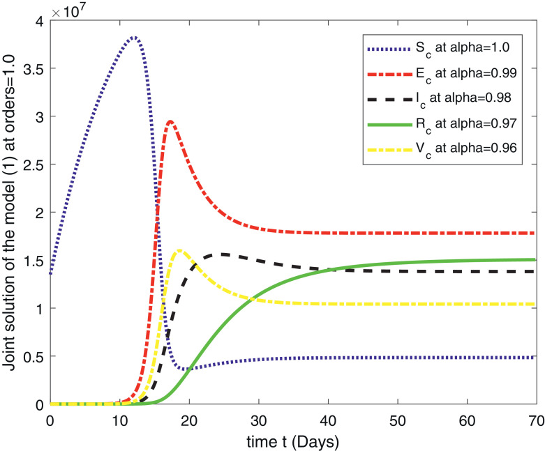
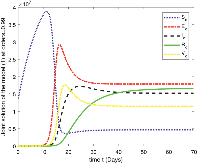
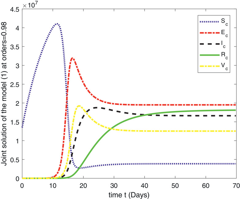
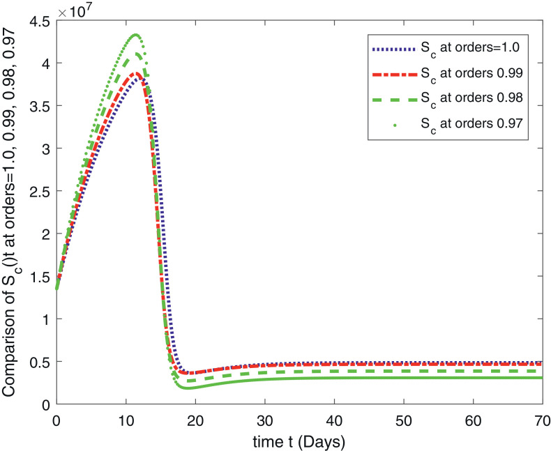
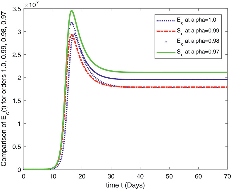
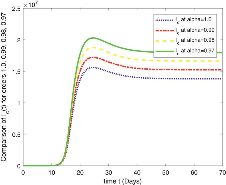
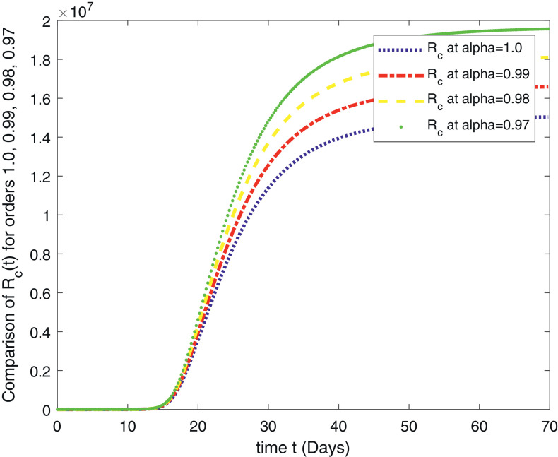
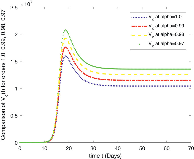
In Fig. 1 , we have given the solution of ABC-Covid-19 model for the ${\kappa }_i=1.0$, for $i=1,2,\dots ,6$. The second Fig. 2 is the solution of the system for the ${\kappa }_i=0.99$, for $i=1,2,\dots ,6$. The third Fig. 3 , represents the solution of the fractional order model (1) for the ${\kappa }_i=0.98$, for $i=1,2,\dots ,6$. The fourth Fig. 4 represent the comparison of the susceptible people $S_c\left(t\right)$ for ${\kappa }_i=\kappa =1.0,0.99,0.98,0.97,0.96$, for $i=1,2,\dots ,6$. This class shows that initially this class is increasing and after 10 days there comes a rapid decrease in the population which is ultimately transferred to the exposed class $E_c\left(t\right)$ given in Fig. 5 and to the infection class $I_c\left(t\right)$ given in Fig. 6 . Figure 7 gives us the detail of the recovery which starts after 15 days and increases in the next upcoming days. In Fig. 8 , the population of the virus is given for the ${\kappa }_i=\kappa =1.0,0.99,0.98,0.97,0.96$, for $i=1,2,\dots ,6$.

Fig. 1.

Joint solution of the fractal-fractional model (1) for ${\kappa }_i^{*}=1.0$, for $i=1,2,\dots ,6$.

Fig. 2.

Joint solution of the fractal-fractional model (1) for ${\kappa }_i^{*}=0.99$, for $i=1,2,\dots ,6$.

Fig. 3.

Joint solution of the fractal-fractional model (1) for ${\kappa }_i^{*}=0.98$, for $i=1,2,\dots ,6$.

Fig. 4.

Comparison of $S_c\left(t\right)$ for ${\kappa }_i^{*}=1.0,0.99,0.98,0.97,0.96$, for $i=1,2,\dots ,6$.

Fig. 5.

Comparison of $E_c\left(t\right)$ for ${\kappa }_i^{*}=1.0,0.99,0.98,0.97,0.96$, for $i=1,2,\dots ,6$.

Fig. 6.

Comparison of $I_c\left(t\right)$ for ${\kappa }_i^{*}=1.0,0.99,0.98,0.97,0.96$, for $i=1,2,\dots ,6$.

Fig. 7.

Comparison of $R_c\left(t\right)$ for ${\kappa }_i^{*}=1.0,0.99,0.98,0.97,0.96$, for $i=1,2,\dots ,6$.

Fig. 8.

Comparison of $V_c\left(t\right)$ for ${\kappa }_i^{*}=1.0,0.99,0.98,0.97,0.96$, for $i=1,2,\dots ,6$.

6. Conclusions

In this paper, we have given an analytical and computational study of the fractional order COVID-19 model (1) for the existence results and numerical simulations. The model is analyzed for the fractional orders ${\kappa }_i=\kappa =1.0,0.99,0.98,0.97,0.96$, for $i=1,2,\cdots ,6$. A computational scheme is derived for the numerical simulation based on the Lagrange’s interpolation polynomial and is tested for the available data given in [14]. The results are graphical represented in eight figures. In Fig. 1, we have given the solution of the fractional order ABC-Covid-19 model for the ${\kappa }_i=1.0$, for $i=1,2,\dots ,6$. The second Fig. 2 is the solution of the system for the ${\kappa }_i=0.99$, for $i=1,2,\dots ,6$. The third Fig. 3, represents the solution of the fractional order model (1) for the ${\kappa }_i=0.98$, for $i=1,2,\dots ,6$. The fourth Fig. 4 represent the comparison of the susceptible people $S_c\left(t\right)$ for ${\kappa }_i=\kappa =1.0,0.99,0.98,0.97,0.96$, for $i=1,2,\dots ,6$. This class shows that initially this class is increasing and after 10 days there comes a rapid decrease in the population which is ultimately transferred to the exposed class $E_c\left(t\right)$ given in Fig. 5 and to the infection class $I_c\left(t\right)$ given in Fig. 6. Figure 7 gives us the detail of the recovery which starts after 15 days and increases in the next upcoming days. In Fig. 8, the population of the virus is given for the ${\kappa }_i=\kappa =1.0,0.99,0.98,0.97,0.96$, for $i=1,2,\dots ,6$. All the results show similar behavior as the classical. For the future study, we suggest the readers for reconsideration of the problem for the optimal control and sensitivity analysis. Also, one can compare the obtained results with the simulations for other fractional derivatives.

Availability of data and material

Not applicable.

CRediT authorship contribution statement

Hasib Khan: Conceptualization, Data curation, Formal analysis, Investigation, Methodology, Software, Visualization, Writing - original draft, Writing - review & editing. Muhammad Ibrahim: Conceptualization, Data curation, Formal analysis, Investigation, Methodology, Software, Visualization, Writing - original draft, Writing - original draft, Writing - review & editing. Abdel-Haleem Abdel-Aty: Conceptualization, Formal analysis, Funding acquisition, Investigation, Project administration, Validation, Visualization, Writing - original draft, Writing - review & editing. M. Motawi Khashan: Conceptualization, Funding acquisition, Investigation, Validation, Visualization, Writing - original draft, Writing - review & editing. Farhat Ali Khan: Conceptualization, Data curation, Investigation, Methodology, Validation, Visualization, Writing - original draft, Writing - review & editing. Aziz Khan: Conceptualization, Data curation, Formal analysis, Investigation, Methodology, Software, Validation, Visualization, Writing - original draft, Writing - review & editing.

Declaration of Competing Interest

The authors have no conflict of interests regarding the publication of this paper.

References

- 1.World Health Organization. Novel coronavirus-China. 2020. URL: https://www.who.int/csr/don/12-january-2020-novel-coronavirus-china/en.
- 2.Kong J.D., Tekwa E., Gignoux-Wolfsohn S. Social, economic, and environmental factors influencing the basic reproduction number of COVID-19 across countries. MedRxiv. 2021 doi: 10.1371/journal.pone.0252373. [DOI] [PMC free article] [PubMed] [Google Scholar]; Jan 1
- 3.World Health Organization . situation report, 72. 2019. Coronavirus disease (COVID-19) [Google Scholar]
- 4.Adhikari S.P., Meng S., Wu Y.J., Mao Y.P., Ye R.X., Wang Q.Z., et al. Epidemiology, causes, clinical manifestation and diagnosis, prevention and control of coronavirus disease (COVID-19) during the early outbreak period: a scoping review. Infect Dis Poverty. 2020;9(1):1–2. doi: 10.1186/s40249-020-00646-x. [DOI] [PMC free article] [PubMed] [Google Scholar]
- 5.Ming W.K., Huang J., Zhang C.J. Breaking down of healthcare system: mathematical modelling for controlling the novel coronavirus (2019-nCoV) outbreak in Wuhan, China. bioRxiv. 2020 [Google Scholar]; Jan 1
- 6.Ferguson N.M., Cummings D.A., Fraser C., Cajka J.C., Cooley P.C., Burke D.S. Strategies for mitigating an influenza pandemic. Nature. 2006;442(7101):448–452. doi: 10.1038/nature04795. [DOI] [PMC free article] [PubMed] [Google Scholar]
- 7.Cowling B.J., Ho L.M., Leung G.M. Effectiveness of control measures during the SARS epidemic in Beijing: a comparison of the Rt curve and the epidemic curve. Epidemiol Infect. 2008;136(4):562–566. doi: 10.1017/S0950268807008722. [DOI] [PMC free article] [PubMed] [Google Scholar]
- 8.Goufo E.F., Pene M.K., Mugisha S. Stability analysis of epidemic models of Ebola hemorrhagic fever with non-linear transmission. J Nonlin Sci Appl. 2016;1(9):4191–4205. [Google Scholar]
- 9.Trauer J.M., Denholm J.T., McBryde E.S. Construction of a mathematical model for tuberculosis transmission in highly endemic regions of the Asia-Pacific. J Theor Biol. 2014;7(358):74–84. doi: 10.1016/j.jtbi.2014.05.023. [DOI] [PubMed] [Google Scholar]
- 10.Ullah I., Ahmad S., Al-Mdallal Q., Khan Z.A., Khan H., Khan A. Stability analysis of a dynamical model of tuberculosis with incomplete treatment. Adv Differ Equ. 2020;2020(1):1–4. [Google Scholar]
- 11.Okuonghae D. A mathematical model of tuberculosis transmission with heterogeneity in disease susceptibility and progression under a treatment regime for infectious cases. Appl Math Modell. 2013;1;37(10–11):6786–6808. [Google Scholar]
- 12.Khan M.A., Atangana A., Alzahrani E. The dynamics of COVID-19 with quarantined and isolation. Adv Differ Equ. 2020;2020(1):1–22. doi: 10.1186/s13662-020-02882-9. [DOI] [PMC free article] [PubMed] [Google Scholar]
- 13.Owolabi K.M., Atangana A. On the formulation of Adams-Bashforth scheme with Atangana-Baleanu-Caputo fractional derivative to model chaotic problems. Chaos. 2019;29(2):023111. doi: 10.1063/1.5085490. [DOI] [PubMed] [Google Scholar]; 7
- 14.Yadav R.P., Verma R. A numerical simulation of fractional order mathematical modeling of COVID-19 disease in case of Wuhan China. Chaos Solitons Fractals. 2020;140:110124. doi: 10.1016/j.chaos.2020.110124. [DOI] [PMC free article] [PubMed] [Google Scholar]
- 15.Atangana A., Araz S.I. Mathematical model of COVID-19 spread in Turkey and South Africa: theory, methods, and applications. Adv Differ Equ. 2020;2020(1):1–89. doi: 10.1186/s13662-020-03095-w. [DOI] [PMC free article] [PubMed] [Google Scholar]
- 16.Atangana A., Araz S.I. Nonlinear equations with global differential and integral operators: existence, uniqueness with application to epidemiology. Results Phys. 2020;21:103593. [Google Scholar]
- 17.Owolabi K.M., Atangana A. On the formulation of Adams-Bashforth scheme with Atangana-Baleanu-Caputo fractional derivative to model chaotic problems. Chaos. 2019;29(2):023111. doi: 10.1063/1.5085490. [DOI] [PubMed] [Google Scholar]; 7
- 18.Gomez J.F., Torres L., Escobar R.F. Springer International Publishing; 2019. Fractional derivatives with Mittag-Leffler kernel. [Google Scholar]
- 19.Atangana A., Baleanu D. New fractional derivatives with nonlocal and non-singular kernel: theory and application to heat transfer model. Therm Sci. 2016;20(2):763–769. doi: 10.2298/TSCI160111018A. [DOI] [Google Scholar]; Jan 20.
- 20.Khan A., Khan H., Gomez-Aguilar J.F., Abdeljawad T. Existence and Hyers-Ulam stability for a nonlinear singular fractional differential equations with Mittag-Leffler kernel. Chaos Solitons Fractals. 2019;127:422–427. [Google Scholar]
- 21.Khan H., Jarad F., Abdeljawad T., Khan A. A singular ABC-fractional differential equation with p-Laplacian operator. Chaos Solitons Fractals. 2019;129:56–61. [Google Scholar]
- 22.Khan A., Gomez-Aguilar J.F., Khan T.S., Khan H. Stability analysis and numerical solutions of fractional order HIV/AIDS model. Chaos Solitons Fractals. 2019;122:119–128. [Google Scholar]
- 23.Khan A., Khan H., Gomez-Aguilar J.F., Abdeljawad T. Existence and Hyers-Ulam stability for a nonlinear singular fractional differential equations with Mittag-Leffler kernel. Chaos Solitons Fractals1. 2019;127:422–427. [Google Scholar]
- 24.Khan H., Gomez-Aguilar J.F., Alkhazzan A., Khan A. A fractional order HIV-TB coinfection model with nonsingular Mittag-Leffler law. Math Methods Appl Sci. 2020;43(6):3786–3806. [Google Scholar]
- 25.Srivastava H.M., Saad K.M., Khader M.M. An efficient spectral collocation method for the dynamic simulation of the fractional epidemiological model of the Ebola virus. Chaos Solitons Fractals. 2020;140:110174. doi: 10.1016/j.chaos.2020.110174. [DOI] [PMC free article] [PubMed] [Google Scholar]
- 26.Alomari A.K., Abdeljawad T., Baleanu D., Saad K.M., Al-Mdallal Q.M. Numerical methods for partial differential equations. 2020. Numerical solutions of fractional parabolic equations with generalized Mittag-Leffler kernels. [Google Scholar]
- 27.Saad K.M., Alqhtani M. Numerical simulation of the fractal-fractional reaction diffusion equations with general nonlinear. AIMS Math. 2021;6(4):3788–3804. [Google Scholar]
- 28.Singh H. Analysis for fractional dynamics of Ebola virus model. Chaos Solitons Fractals. 2020;138:109992. doi: 10.1016/j.chaos.2020.109992. [DOI] [PMC free article] [PubMed] [Google Scholar]
- 29.Singh H. Analysis of drug treatment of the fractional HIV infection model of CD4+ t-cells. Chaos Solitons Fractals. 2021;146:110868. [Google Scholar]
- 30.Singh H., Srivastava H.M. Numerical simulation for fractional-order Bloch equation arising in nuclear magnetic resonance by using the Jacobi polynomials. Appl Sci. 2020;10(8):2850. [Google Scholar]
- 31.Singh H., Srivastava H.M., Hammouch Z., Nisar K.S. Numerical simulation and stability analysis for the fractional-order dynamics of COVID-19. Results Phys. 2021;20:103722. doi: 10.1016/j.rinp.2020.103722. [DOI] [PMC free article] [PubMed] [Google Scholar]
- 32.Singh H., Baleanu D., Singh J., Dutta H. Computational study of fractional order smoking model. Chaos Solitons Fractals. 2021;142:110440. [Google Scholar]
- 33.Panwar V.S., Uduman P.S., Gomez-Aguilar J.F. Mathematical modeling of coronavirus disease COVID-19 dynamics using CF and ABC non-singular fractional derivatives. Chaos Solitons Fractals. 2021;145:110757. doi: 10.1016/j.chaos.2021.110757. [DOI] [PMC free article] [PubMed] [Google Scholar]
- 34.Nabi K.N., Kumar P., Erturk V.S. Projections and fractional dynamics of COVID-19 with optimal control strategies. Chaos Solitons Fractals. 2021;145:110689. doi: 10.1016/j.chaos.2021.110689. [DOI] [PMC free article] [PubMed] [Google Scholar]
Associated Data
This section collects any data citations, data availability statements, or supplementary materials included in this article.
Data Availability Statement