Discrete and continuum models of COVID-19 virus, formal solutions, stability and comparison with real data

Abstract

Very recently, various mathematical models, for the dynamics of COVID-19 with main contribution of suspected–exposed–infected–recovered people have been proposed. Some models that account for the deceased, quarantined or social distancing functions were also presented. However, in any local space the real data reveals that the effects of lock-down and traveling are significant in decreasing and increasing the impact of this virus respectively. Here, discrete and continuum models for the dynamics of this virus are suggested. The continuum dynamical model is studied in detail. The present model deals with exposed, infected, recovered and deceased individuals (EIRD), which accounts for the health isolation and travelers (HIT) effects. Up to now no exact solutions of the parametric-dependent, nonlinear dynamical system NLDS were found. In this work, our objective is to find the exact solutions of a NLDS. To this issue, a novel approach is presented where a NLDS is recast to a linear dynamical system LDS. This is done by implementing the unified method (UM), with auxiliary equations, which are taken coupled linear ODE’s (LDS). Numerical results of the exact solutions are evaluated, which can be applied to data in a local space (or anywhere) when the initial data for the IRD are known. Here, as an example, initial conditions for the components in the model equation of COVID-19, are taken from the real data in Egypt. The results of susceptible, infected, recovered and deceased people are computed. The comparison between the computed results and the real data shows an agreement up to a relative error $10^{-3}$. On the other hand it is remarked that locking-down plays a dominant role in decreasing the number of infected people. The equilibrium states are determined and it is found that they are stable. This reveals a relevant result that the COVID-19 can be endemic in the case of a disturbance in the number of the exposed people. A disturbance in the form of an increase in the exposed number, leads to an increase in the number of infected people. This result is, globally, valid. Furthermore, initial states control is analyzed, where region of initial conditions for infected and exposed is determined. We developed a software tool to interact with the model and facilitate applying various data of different local spaces.

1. Introduction

Corona viruses belong to the Corona viridae family in the Nidovirales order. Corona represents crown-like spikes on the outer surface of the virus [4]. COVID-19 virus received the attention of many research works in science and medicine [4], [16].

It is evident that this virus is transmitted between people through respiratory droplets and contact routes [6], [15], [18], [21]. It occurs when a person is in close contact (within 1 m) with someone who has respiratory symptoms and is therefore at risk of having his/her mouth and nose exposed to potentially infective respiratory droplets. Estimation of the asymptomatic ratio, the percentage of carriers with no symptoms, will improve understanding of the virus transmission [14].

The application of a recent epidemiological model, suspected–exposed–infected–recovered, namely SEIR with Social Distancing (SEIR-SD), is extended here through the definition of a social distancing function varying over time to assess the situation related to the spreading of the COVID-19 in Italy [7], [20]. In this work, the most suitable values of its parameters are found. Due to Egypt’s high population density, human to human social contact rate is very high. So, control of the pandemic COVID-19 is very urgent in the early stage and is a challenging problem. Several mathematical models were proposed to study the COVID-19 dynamics and also to identify the influential parameters that leads to reduce the outbreak size [5]. A model was proposed in [17] that takes into account the combination of a global network mobility model with a local epidemiology model to simulate and predict the outbreak dynamics and outbreak control of COVID-19 across Europe. A stochastic transmission model was developed [11] by extending the Susceptible–Infected–Removed (SIR) that assesses the effectiveness of response strategies of avoiding crowded areas and predicts the spread of COVID-19 infections in Japan. The outbreak of COVID-19 disease in mainland China was characterized by a distinctive sub-exponential increase of confirmed cases during the early phase of the epidemic, contrasting with an initial exponential growth expected for an unconstrained outbreak. This effect has been taken into consideration in [19]. The longtime of quarantine is expensive, so to study the optimal control problems of cost-effective quarantine strategies, a formulation of two control SEIR-type models describing the spread of the COVID-19 in a human population was considered in [8], [12], [13], [13].

2. The model and formal exact solutions

2.1. Discrete and continuum models

We propose a EIRD-HIT model by the difference equations:

$$\begin{array}{c}\hfill E_{n+1}=(1-\sigma )E_n-\frac{\alpha E_n{I}_n}{N}+k_1,\hfill \\ \hfill I_{n+1}=(1-\beta -\gamma )I_n+\frac{\alpha E_n{I}_n}{N}+k_2,\hfill \\ \hfill R_{n+1}=R_n+\beta I_n,\hfill \\ \hfill D_{n+1}=D_n+\gamma I_n.\hfill \end{array},$$ (1)

By using (1), the continuum model is constructed as in what follows. We write

$$E_n=E\left(t\right),E_{n+1}=E(t+1)\approx E\left(t\right)+\frac{dE\left(t\right)}{dt},$$ (2)

and similar equations for $I_n,R_n$, and $D_n$ hold. Thus, we have

$$\begin{array}{c}\hfill \frac{dE\left(t\right)}{dt}=(-\sigma E\left(t\right)-\frac{\alpha E\left(t\right)I\left(t\right)}{N}+k_1),\hfill \\ \hfill \frac{I\left(t\right)}{dt}=(-\sigma I\left(t\right)+\frac{\alpha E\left(t\right)I\left(t\right)}{N}+k_2),\hfill \\ \hfill \frac{dR\left(t\right)}{dt}=\beta I\left(t\right),\hfill \\ \hfill \frac{dD\left(t\right)}{dt}=\gamma I\left(t\right),\hfill \end{array}$$ (3)

where

(a) $\alpha$ is the rate of exposed people to infection.

(b) $\sigma$ is the rate of isolated people.

(c) $\beta$ and $\gamma$ are the rates of the interaction of recovered and deceased with the infected people respectively.

(d) $k_1$ and $k_2$ are the pumping rates of exposed and infected travelers respectively.

(e) $N$ is the population number.

Indeed, a model which is more realistic than what is presented in (3), is to take into consideration the fact that diseased or recovered people were antecedent infected. Thus a delay time has to be introduced in the last two equations in (3) in $I\left(t\right)$. Thus the model in (3) becomes

$$\begin{array}{c}\hfill \frac{dE\left(t\right)}{dt}=(-\sigma E\left(t\right)-\frac{\alpha E\left(t\right)I\left(t\right)}{N}+k_1),\hfill \\ \hfill \frac{I\left(t\right)}{dt}=(-\sigma I\left(t\right)+\frac{\alpha E\left(t\right)I\left(t\right)}{N}+k_2),\hfill \\ \hfill \frac{dR\left(t\right)}{dt}=\beta I(t-{\tau }_1),\hfill \\ \hfill \frac{dD\left(t\right)}{dt}=\gamma I(t-{\tau }_2),\hfill \end{array}$$ (4)

where ${\tau }_1$ and ${\tau }_2$ are the measures of time lag between infection and recovered/deceased.

It is worthy to mention that a nonlinear dynamical system is not in general integrable. It may be conditionally integrable. This holds in the present case and the condition for integrability will be depicted later on.

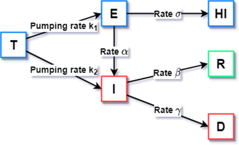
The scheme of the model is shown in Fig. 1.

Fig. 1.

Presented model.

2.2. Exact solutions

The unified method, used here, asserts that the exact solutions of NLDS are expressed in auxiliary functions which satisfy appropriate auxiliary equations. Here, these later equations are taken as linear coupled ODEs, which may be considered as LDS.

Now, in (4) when $I\left(t\right)$ is known, then we get

$$R\left(t\right)=R\left({\tau }_1\right)+\beta {\int }_{{\tau }_1}^{t}I(t_1-{\tau }_1)d{t}_1,D\left(t\right)=D\left({\tau }_2\right)+\gamma {\int }_{{\tau }_2}^{t}I(t_1-{\tau }_2)d{t}_1.$$ (5)

Thus, we are left with first and second equations in (4), which will be solved, hereafter. Here we find the exact solutions by using the UM [1], [2], [3], where the solutions are expressed in the rational form by

$$\begin{array}{c}\hfill E\left(t\right)=\frac{R_1}{Q},I\left(t\right)=\frac{R_2}{Q},R_1=a_0+\sum _1^3{a}_j{g}_j\left(t\right)\hfill \\ \hfill R_2=b_0+\sum _1^3{b}_j{g}_j\left(t\right),Q=s_0+\sum _1^3{s}_j{g}_j\left(t\right),\hfill \end{array}$$ (6)

where $g_j\left(t\right),j=1,2,3$ are the auxiliary functions which satisfy the auxiliary equations,

$$\begin{array}{c}\hfill \frac{d{g}_1\left(t\right)}{dt}=\sum _1^3{\alpha }_j{g}_j\left(t\right),\frac{d{g}_2\left(t\right)}{dt}=\sum _1^3{\beta }_j{g}_j\left(t\right),\hfill \\ \hfill \frac{d{g}_3\left(t\right)}{dt}=\sum _1^3{\gamma }_j{g}_j\left(t\right).\hfill \end{array}$$ (7)

By substituting from (6), (7) into the first and second equations in (3), and by setting the coefficients of $g_j^k,j=1,2,3,k=0,1,2,.$., equal to zero, we get a set of algebraic equations which solve to

$$\begin{array}{c}\hfill b_0=-\frac{1}{s_3\alpha }{s}_0(-a_3\alpha +N(2s_2{\beta }_3+s_3(\beta +\gamma +2{\gamma }_3))),\hfill \\ \hfill \hfill \\ \hfill k_2=-\frac{1}{N{s}_3^2\alpha }(-a_3\alpha +N{s}_3(\beta +\gamma ))(-a_3\alpha +N(2s_2{\beta }_3+s_3(\beta +\gamma +2{\gamma }_3))),\hfill \\ \hfill \hfill \\ \hfill b_1=-\frac{1}{s_3\alpha }(-2a_3{s}_1\alpha +a_1{s}_3\alpha +N{s}_1(2s_2\beta +s_3(\beta +\gamma +2\gamma ))),\hfill \\ \hfill \hfill \\ \hfill a_2=\frac{1}{s_1{\beta }_3}(a_1{s}_2\beta -a_3{s}_1\gamma +a_1{\gamma }_3),b_3=\frac{1}{\alpha }(a_3\alpha -N(2s_2{\beta }_3+s_3(\beta +\gamma +2{\gamma }_3))),\hfill \\ \hfill \hfill \\ \hfill {\gamma }_1=\frac{1}{N{s}_3^2}(a_3{s}_1\alpha -a_1{s}_3\alpha -N{s}_1(2s_2{\beta }_3+s_3{\gamma }_3)),\sigma =\beta +\gamma ,\hfill \\ \hfill \hfill \\ \hfill b_2=\frac{1}{s_1{s}_3\alpha {\beta }_3}\text{(}-a_1{s}_3\alpha (s_2{\beta }_3+s_3{\gamma }_3)+a_3{s}_1\alpha \text{(}2s_2{\beta }_3+s_3{\gamma }_3\hfill \\ \hfill -N{s}_1{s}_2{\beta }_3(2s_2{\beta }_3+s_3(\beta +\gamma +2{\gamma }_3))\text{))},\hfill \\ \hfill \hfill \\ \hfill {\alpha }_2=\frac{{(s_2{\beta }_3+s_3{\gamma }_3)}^2}{s_1{s}_3{\beta }_3},{\alpha }_1={\beta }_2,{\beta }_2=\frac{s2{\beta }_3}{s_3}+{\gamma }_3,{\beta }_1=\frac{s_1{\beta }_3}{s_3},\hfill \\ \hfill {\alpha }_3=-\frac{1}{s_1}(s_2{\beta }_3+s_3{\gamma }_3),\hfill \\ \hfill {\gamma }_2=-\frac{1}{N{s}_1{s}_3^2{\beta }_3}(s_2{\beta }_3+s_3{\gamma }_3)(-a_3{s}_1\alpha +a_1{s}_3\alpha +N{s}_1(2s_2{\beta }_3+s_3{\gamma }_3)),\hfill \end{array}$$ (8)

together with the condition of integrability which is $\sigma =\beta +\gamma$, which leads to $\sigma >\beta$ and $\sigma >\gamma$. Thus this condition has an impact on the dynamics of COVID-19, in the sense that the rate of isolated people should be greater than the rate of recovery and of diseased people.

The solutions of the auxiliary equations (7) are

$$\begin{array}{c}\hfill g_1\left(t\right)=\frac{P_1}{2Q_1},g_2\left(t\right)=\frac{P_2}{2Q_1},g_3\left(t\right)=\frac{P_3}{Q_1},\hfill \\ \hfill \hfill \\ \hfill P_1=a_3{s}_1{\alpha }_2(-1+e^{t{\gamma }_3}{s}_2{\beta }_3+(-1+2e^{t{\gamma }_3}-e^{2t(\frac{s_2{\beta }_3}{s_3}+{\gamma }_3)})s_3{\gamma }_3)K\hfill \\ \hfill +a_1{s}_3\alpha -2(-1+e^{t{\gamma }_3}{s}_2{\beta }_3+(1-2e^{t{\gamma }_3}+e^{2t(\frac{s_2{\beta }_3}{s_3}+{\gamma }_3)})s_3{\gamma }_3)K\hfill \\ \hfill -2N{s}_1(2s_2{\beta }_3+s_3{\gamma }_3)\text{(}{s}_1{\beta }_3\text{((}-1+e^{t{\gamma }_3}{s}_2{\beta }_3+(-1+e^{t{\gamma }_3})-\hfill \\ \hfill e^{2t(\frac{s_2{\beta }_3}{s_3}+{\gamma }_3)}\text{)}{s}_3{\gamma }_3\text{)}{g}_1\left(0\right)+(s_2{\beta }_3+s_3{\gamma }_3)\text{((}-1+e^{t{\gamma }_3}{s}_2{\beta }_3{g}_2\left(0\right)+s_3\text{(}-e^{2t(\frac{s_2{\beta }_3}{s_3}+{\gamma }_3)}{g}_2\left(0\right)\hfill \\ \hfill -{\beta }_3{g}_3\left(0\right)+e^{t{\gamma }_3}({\gamma }_3{g}_2\left(0\right)+{\beta }_3{g}_3\left(0\right))\text{))))},\hfill \\ \hfill \hfill \\ \hfill P_2=(-a_3{s}_1\alpha (2(-1+e^{t{\gamma }_3})s_2{\beta }_3+(-1+2e^{t{\gamma }_3})-e^{2t(\frac{s_2{\beta }_3}{s_3}+{\gamma }_3)})s_3{\gamma }_3)K\hfill \\ \hfill +a_1{s}_3\alpha 2(-1+e^{t{\gamma }_3}{s}_2{\beta }_3+(-1+2e^{t{\gamma }_3}-e^{2t(\frac{s_2{\beta }_3}{s_3}+{\gamma }_3)})s_3{\gamma }_3)K\hfill \\ \hfill +2N{s}_1(2s_2^2{\beta }_3^2+3s_2{s}_3{\beta }_3{\gamma }_3+s_3^2{\gamma }_3^2)-1+e^{t{\gamma }_3}{s}_1{\beta }_3{g}_1\left(0\right)\hfill \\ \hfill +(-1+e^{t{\gamma }_3})s_2{\beta }_3{g}_2\left(0\right)+s_3\text{(}-{\beta }_3{g}_3\left(0\right)+e^{t{\gamma }_3}(\gamma g_2\left(0\right)+{\beta }_3{g}_3\left(0\right)),\hfill \\ \hfill \hfill \\ \hfill P_3=\text{(}a3e^{t{\gamma }_3}(-1+e^{2t(\frac{s_2{\beta }_3}{s_3}+{\gamma }_3)})s_1\alpha (s_1{\beta }_3{g}_1\left(0\right)+(s_2{\beta }_3+s_3{\gamma }_3)g_2\left(0\right))\hfill \\ \hfill +a_1(e^{t{\gamma }_3}-e^{2t(\frac{s_2{\beta }_3}{s_3}+{\gamma }_3)})K+e^{t{\gamma }_3}\text{)}N{s}_1(2s_2{\beta }_3+s_3{\gamma }_3)\text{(}-(-1+e^{2t(\frac{s_2{\beta }_3}{s_3}+{\gamma }_3)})s_1{\beta }_3{g}_1\left(0\right)\hfill \\ \hfill -(-1+e^{2t(\frac{s_2{\beta }_3}{s_3}+{\gamma }_3)})s_2{\beta }_3{g}_2\left(0\right)+s3(-(-1+e^{2t(\frac{s_2{\beta }_3}{s_3}+{\gamma }_3)}){\gamma }_3\left(0\right)+{\beta }_3{g}_3\left(0\right))\text{))},\hfill \\ \hfill \hfill \\ \hfill K=(s_1{\beta }_3{g}_1\left(0\right)+(s_2{\beta }_3+s3{\gamma }_3)g_2\left(0\right)),Q_1=N{s}_1{s}_3{\beta }_3(2s_2{\beta }_3+s_3{\gamma }_3).\hfill \end{array}$$ (9)

By substituting From (8), (9) into (6), we get

$$\begin{array}{c}\hfill E\left(t\right)=\frac{R_1}{Q},I\left(t\right)=-\frac{R_2}{\alpha Q},\hfill \\ \hfill \hfill \\ \hfill R_1=a_3^2(-1+e^{2t(\frac{s_2{\beta }_3}{s_3}+{\gamma }_3)})\alpha +2e^{2t(\frac{s_2{\beta }_3}{s_3}+{\gamma }_3)}N{s}_3(s_2{\beta }_3+s_3{\gamma }_3)E\left(0\right)\hfill \\ \hfill -a_3(-1+e^{2t(\frac{s_2{\beta }_3}{s_3}+{\gamma }_3)})(2N(s_2{\beta }_3+s_3{\gamma }_3)+s_3\alpha E\left(0\right)),\hfill \\ \hfill \hfill \\ \hfill R_2=-a_3^2(-1+e^{2t(\frac{s_2{\beta }_3}{s_3}+{\gamma }_3)}){\alpha }^2+a_3\alpha \text{(}N(-4s_2{\beta }_3+s_3((-1+e^{2t(\frac{s_2{\beta }_3}{s_3}+{\gamma }_3)})(\beta +\gamma )-4{\gamma }_3))\hfill \\ \hfill +(-1+e^{2t(\frac{s_2{\beta }_3}{s_3}+{\gamma }_3)})s_3\alpha E\left(0\right)\text{)}+N\text{(}2N(s_2{\beta }_3+s_3{\gamma }_3)(2s_2{\beta }_3+s_3(\beta +\gamma +2{\gamma }_3))\hfill \\ \hfill +s_3\alpha (2s_2{\beta }_3+s_3((1-e^{2t(\frac{s_2{\beta }_3}{s_3}+{\gamma }_3)})(\beta +\gamma )+2{\gamma }_3))E\left(0\right)\text{)},\hfill \\ \hfill \hfill \\ \hfill Q=\left(s_3\alpha (a_3(-1+e^{2t(\frac{s_2{\beta }_3}{s_3}+{\gamma }_3)})\alpha +2N(s_2{\beta }_3+s_3{\gamma }_3)-(-1+e^{2t(\frac{s_2{\beta }_3}{s_3}+{\gamma }_3)})s_3\alpha E\left(0\right))\right),\hfill \end{array}$$ (10)

together with

$$\begin{array}{c}\hfill a_0=\frac{s_0}{2\alpha \sigma }\left(\alpha (k_1+k_2)+N{(\beta +\gamma )}^2+\sqrt{-4k_{1}N\alpha {(\beta +\gamma )}^2+{(\alpha (k_1+k_2)+N{(\beta +\gamma )}^2)}^2}\right)\hfill \\ \hfill \hfill \\ \hfill a_3=\frac{1}{a_0\alpha }{s}_3(-k_{1}N{s}_0+a_0(N(\beta +\gamma )+\alpha (E\left(0\right)+I\left(0\right)))),\hfill \\ \hfill \hfill \\ \hfill {\gamma }_3=\frac{1}{2a_{0}N{s}_3}(-2k_{1}N{s}_3{s}_0+a_0(N{s}_3(\beta +\gamma )-2N{s}_2{\beta }_3+s_3\alpha (E\left(0\right)+I\left(0\right)))).\hfill \end{array}$$ (11)

We mention that when substituting from (11), for $a_0$, $a_3$ and ${\gamma }_3$, into (10), the results obtained are very lengthy to be produced here.

3. Numerical results

To adapt the model for any country data:

• 1.Given the EIRD real data for a specific local space starting from the initial values and covering a certain period of time.
• 2.Experiment with these real data to find the order of magnitude of the best-fit for the $\beta$, $\gamma$, $\alpha$, $k_1$, and $k_2$ in Eq. (3).
• 3.Use the values of these parameters to predict the EIRD for a longer period of time.

When the above steps were carried on the real data of Egypt, starting from March 1st to August 30th, 2020, we found that

$$\sigma =O\left(\beta \right),\gamma \ll \alpha E\left(0\right)/N,N=10^8,$$ (12)

where $N$ is the population number of Egypt.

The exact solutions in (10), (11) are evaluated numerically. The initial values are taken after the real data in Egypt at the starting date, where the infected and deceased people are 226 and 6 respectively. Thus the initial values are $I\left(0\right)=225$ and $D\left(0\right)=6$. The initial values of $g\left(0\right),i=1,2,3$ are evaluated, which depend on $E\left(0\right)$ and $I\left(0\right)$. We have

$$\begin{array}{c}\hfill g_3\left(0\right)=\frac{1}{s_1{s}_3{\beta }_3(-a_3+s_{3}E\left(0\right))}{a}_3{s}_1(s_0{\beta }_3-s_3{\gamma }_3{g}_2\left(0\right))+s_3\text{(}-s_1^2{\beta }_{3}E\left(0\right)g_1\left(0\right)\hfill \\ \hfill +a_1(s_2{\beta }_3+s_3{\gamma }_3)g_2\left(0\right)-s_1{\beta }_3(s_{0}E\left(0\right)-a_1{g}_1\left(0\right)+s_{2}E\left(0\right)g_2\left(0\right))\text{)},\hfill \end{array}$$ (13)

where $g_1\left(0\right)$ and $g_2\left(0\right)$ are arbitrary. The numerical results for infected, exposed, recovered and deceased people are shown, in what follows up to end of August. In Fig. 2, the number of infected people is displayed against time, in days,

Fig. 2.

(i) and (ii): The variation of the number of infected people is displayed against $t$ when $N=100,000,000$, $I\left(0\right)=226$, $E\left(0\right)=190,000$, $D\left(0\right)=6$, $R\left(0\right)=32$, $k_1=150$, $s_0=0.005$, $s_2=0.9$, $s_3=0.75$, $\beta =0.0048,\gamma \text{=0.0003},$$\sigma =\beta +\gamma$, ${\beta }_3=1.4$.

In (i) $k_2=5$ and for different values of $\alpha$. In (ii) $\alpha =1$ and for different values of $k_2$.

From Fig. 2, we find that the infected people at the end of September will be about $103683$ when $\alpha =1$. After Fig. 2(ii), we remark that the effects of the parameters $k_1$ and $k_2$ are insensitive. This may be argued to the small numerical (moderate) values taken, of these parameters. We think that by taking large numerical values, remarkable effects may hold.

In Fig. 3, the exposed, deceased and recovered are shown.

Fig. 3.

(i), (ii) and (iii): The variation of the exposed, deceased, and recovered numbers with the parameter values as in Fig. 2(i) and (ii). In (i): $k_2=5$. In (ii) and (iii): $\alpha =0.2,{\tau }_1=15,{\tau }_2=10$.

The results in Figs. 2(i), (ii) and 3(i)–(iii), are compared with the real data at the end of September and summarized as shown in Table 1.

It is worth noticing that the parameters $\alpha ,\beta ,\gamma ,\dots$,in (4), are taken appropriately to match with the real data in local spaces.

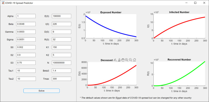
We implemented the final Eqs. ((10) and (11)) as a MATLAB software application to allow researchers to utilize this model for various real data of different countries. The tool can be reached through [9]. Fig. 4 shows a screenshot for the tool.

Fig. 4.

Screenshot for the MATLAB software application for predicting the spread of COVID-19.

A comparison between the method used here and the known methods in the literature is done in the following:

1 — In this paper, the unified method presented in [13] was used. After this nomenclature, this method unifies all known methods such as, the Exp-function expansion [10], [22], the tanh modified, and the extended versions; the F-expansion and the G’/G expansion method.

2 — On the other hand, the extended unified method, proposed in [12], may be sufficient to replace the analysis of using the symmetries by inspecting the symmetries endowed by using Lie group in NLPDEs.

3 — Using the generalized unified method, presented in [1], is more powerful tool than using the Hirota method.

Table 1.

Real data is compared against computed data for Infected, recovered and deceased. In this table, the relative error $=\left|\frac{real-computed}{real}\right|$.

	Real data	Computed data	Relative error
Infected	103 483	103 683	$1.9\times .10^{-3}$
Recovered	97 050	97 320	$3\times .10^{-3}$
Deceased	5930	5923	$.10^{-3}$

4. Stability

The equilibrium states ES are determined by setting the RHS in (3) equal to zero. There exist two ESs,

(i) When $k_2=0$, we have $E_e=k_1/{\sigma }_e=0$ and $I_e=0$.

(ii) When $k_2\ne 0$, we have $E_e=\frac{k_{1}N}{\alpha I_e+N\sigma }$ and $I_e=\frac{1}{2\alpha (\beta +\gamma )}(\alpha (k_1+k_2)-N{(\beta +\gamma )}^2+\sqrt{4k_{2}N{(\beta +\gamma )}^2+{(\alpha (k_1+k_2)-N(\beta +\gamma )\sigma )}^2})$.

We consider the ES in (ii) and assume that $E\left(t\right)=E_e+{\varepsilon }_1{e}^{\lambda t}$ and $I\left(t\right)=I_e+{\varepsilon }_2{e}^{\lambda t}$, by substituting in the first and second equations in (3), we have

$$\begin{array}{c}\hfill M\left(\begin{array}{c}\hfill {\varepsilon }_1\hfill \\ \hfill {\varepsilon }_2\hfill \end{array}\right)=0,M=\left(\begin{array}{cc}\hfill a_{11}\hfill & \hfill a_{12}\hfill \\ \hfill a_{21}\hfill & \hfill a_{22}\hfill \end{array}\right),\hfill \\ \hfill \hfill \\ \hfill a_{21}=-I_e\alpha (I_e\alpha +N(\beta +\gamma )),\hfill \\ \hfill a_{22}=I_{e}N\alpha (\beta +\gamma +\lambda )+k_2{N}^2(k_1\alpha (\beta +\gamma )-N{(\beta +\gamma )}^2(\beta +\gamma +\lambda )).\hfill \end{array}$$ (14)

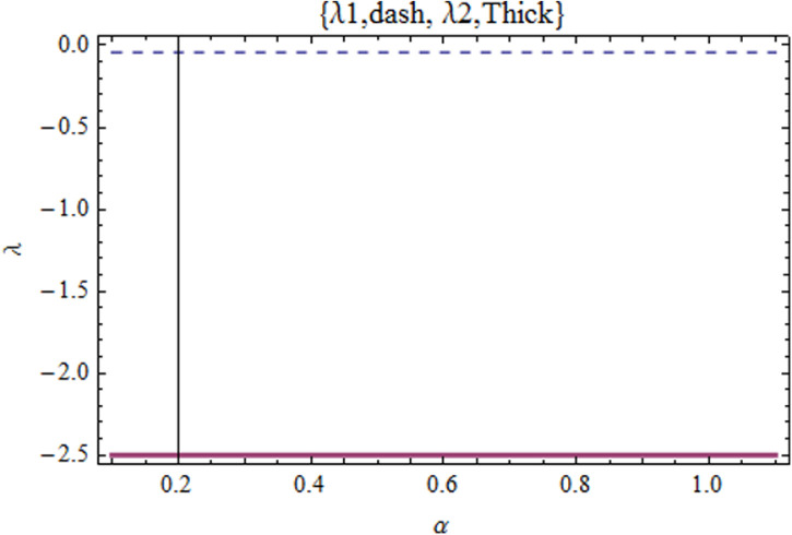
By setting $det$ $\left(M\right)=0$, we get the characteristic equation, which is solved in $\lambda$. The results are lengthy to be produced here. They are shown in Fig. 5 where we find that the ES in the case (ii) is asymptotically stable. By the same way, it is found that the ES in the case (i) is also asymptotically stable. This result leads to that the systems returns to the equilibrium state under disturbance. Or the COVID-19 maybe endemic.

Fig. 5.

The eigenvalues $\lambda$ are displayed against $\alpha$ when $k_1=150$, $k_2=10$, $\beta =0.004$, $\gamma =0.0002$, $N=100000000$.

4.1. Initial state control

The criteria of initial state control asserts that, we can control the number of exposed and infected people such that, initially, the rate of infected people is negative, $\frac{dI\left(t\right)}{dt}{\mid }_{t=0}<0$. By using Eq. (3) we get

$$I\left(0\right)<\frac{N{k}_2}{(\alpha E\left(0\right)-N(\beta +\gamma ))}.$$ (15)

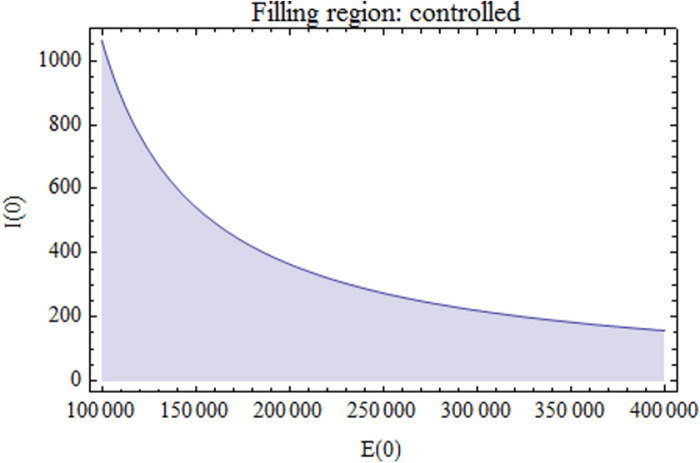
Eq. (15) is shown in figure Fig. 6. As shown, with relevance to the initial values considered, we find that when $I\left(0\right)>1000$ and $E\left(0\right)>400000$, the states are uncontrolled. While they are controlled when they are in the filling region.

Fig. 6.

$I\left(0\right)$ displayed against $E\left(0\right)$ to show the region under control when $\beta =0.004,\gamma =0.00059,k_2=5,N=100000000,\alpha =9$.

4.2. Discussion of the results

The model presented here takes into account of the effects of the number lock-down and travelers people. These were not considered previously. In many works, attention was focused on some local characteristics, relevant to the country under study. Here this is not proposed. Thus, we think that the model equations presented here is global. The exact solutions of the model equation are obtained where the approach presented here is novel. Thus, we are able to compare the results found with the real data which is shown in Table 1.

It is worthy to notice that we can control the parameters $\alpha$, $\beta$, $\gamma$, and $k_i,i=1,2$ to fit the exact solutions with real data in any locality (country).

In fact, in the previous works, only the order of magnitude estimate of each component in a COVID-19 model was done.

A comparison between the method used here and the known methods in the literature is done in the following:

1 — In this paper, the unified method presented in [13] was used. After this nomenclature, this method unifies all known methods such as, the Exp-function expansion [10], [22], the tanh, modified, and the extended versions, the F-expansion, the G’/G expansion method.

2 — On the other hand, the extended unified method, proposed in [12], may be sufficient to replace the analysis of using the symmetries by inspecting the symmetries endowed by using Lie group in NLPDEs.

3 — Using the generalized unified method, presented in [1], is more powerful tool than using the Hirota method.

5. Conclusions

In this work, discrete and continuum models account for the exposed, infected, recovered, deceased, locked-down and travelers, EIRD-HIT, are presented. The exact solutions of the model equations are found by using the unified method with linear coupled auxiliary equations. These solutions are evaluated numerically and the results are compared with the real data in Egypt. On the other hand, it is shown that the dynamic system of COVID-19 is stable. This result shows that a disturbance in the number of exposed people, might lead to the virus becoming endemic. We mention that this model can be applied to arbitrary initial data. In view of the mathematical modeling, the number of infected people does not decrease to zero in the absence of antivirus effect.

CRediT authorship contribution statement

Hamdy I. Abdel-Gawad: Conceptualization,Methodology, Writing – original draft. Ahmed H. Abdel-Gawad: Software, Writing - review & editing.

Declaration of Competing Interest

The authors declare that they have no known competing financial interests or personal relationships that could have appeared to influence the work reported in this paper.

References

- 1.Abdel-Gawad H.I. Towards a unified method for exact solutions of evolution equations. An application to reaction diffusion equations with finite memory transport. J. Stat. Phys. 2012;147:506–521. [Google Scholar]
- 2.Abdel-Gawad H.I., Biswas A. Multi-soliton solutions based on interactions of basic traveling waves with an applications to the nonlocal Boussinesq equation. Acta Phys. Polon. B. 2016;47:1101–1112. [Google Scholar]
- 3.Abdel-Gawad H.I., El-Azab N., Osman M. Exact solution of the space -dependent KdV equation. JPSP. 2013;82 [Google Scholar]
- 4.Adnan M., Suliman S., Khana R., Kazmic A., Bashir N., Siddique R. COVID-19 infection: Origin, transmission, and characteristics of human coronaviruses. J. Adv. Res. 2020;24:91–98. doi: 10.1016/j.jare.2020.03.005. [DOI] [PMC free article] [PubMed] [Google Scholar]
- 5.Biswas S.K., Ghosh J.K., Sarkar S., Ghosh U. 2020. COVID-19 pandemic in India: A mathematical model study. 2020050508. [DOI] [PMC free article] [PubMed] [Google Scholar]
- 6.Chan J., Yuan S., Kok K. A familial cluster of pneumonia associated with the 2019 novel coronavirus indicating person-to-person transmission: a study of a family cluster. Lancet. 2020 doi: 10.1016/S0140-6736(20)30154-9. [DOI] [PMC free article] [PubMed] [Google Scholar]
- 7.De Falco I., Della Cioppa A., Scafuri U., Tarantino E. 2020. Coronavirus Covid-19 spreading in Italy: optimizing an epidemiological model with dynamic social distancing through Differential Evolution. Search Q. Biol, arXiv:2004.00553. [Google Scholar]
- 8.Grigorieva E.V., Khailov A. 2020. Optimal quarantine-strategies for COVID-19 control problems. arXiv:2004.106614v2. [DOI] [PMC free article] [PubMed] [Google Scholar]
- 9.http://www.mathworks.com/matlabcentral/fileexchange/78167-covid-19-spread-predictor-includes-data-for-egypt.
- 10.He Ji-H., Hong X. Exp-function method for nonlinear wave equations. Chaos Solitons Fractals. 2006;30:700–708. [Google Scholar]
- 11.Karako K., Song P., Chen Y., Tang W. Advance Publication; 2020. Analysis of COVID-19 Infection Spread in Japan Based on Stochastic Transition Model. [DOI] [PubMed] [Google Scholar]
- 12.Khan M.A., Atangana A. Modeling the dynamics of novel coronavirus (2019-nCov) with fractional derivative. Alexandria Engineering Journal. 2020;59(4):2379–2389. [Google Scholar]
- 13.Khan M.A., Atangana A., Alzahrani E., Wati F. The dynamics of COVID-19 with quarantined and isolation. Adv. Difference Equ. 2020;2020(1):1–22. doi: 10.1186/s13662-020-02882-9. [DOI] [PMC free article] [PubMed] [Google Scholar]
- 14.Li Q., Guan X., Wu P., Wang X., Zhou L., Tong Y. Early transmission dynamics in Wuhan, China, of novel coronavirus-infected pneumonia. N. Engl. J. Med. 2020;382(13):1199–1207. doi: 10.1056/NEJMoa2001316. [DOI] [PMC free article] [PubMed] [Google Scholar]
- 15.Li Q., Guan X., Wu P. Early transmission dynamics in Wuhan, China, of novel coronavirus-infected pneumonia. N. Engl. J. Med. 2020 doi: 10.1056/NEJMoa2001316. [DOI] [PMC free article] [PubMed] [Google Scholar]
- 16.Li Hua, Liu Zhe, Ge Junbo. 2020. Scientific research progress of COVID-19/SARS-CoV-2 in the first five months. Review. [DOI] [PMC free article] [PubMed] [Google Scholar]
- 17.Linka K., Peirlinck M., Costabal F.S., Kuhl E. 2020. Outbreak dynamics of COVID-19 in Europe and the effect of travel restrictions. [DOI] [PMC free article] [PubMed] [Google Scholar]
- 18.Liu J., Liao X., Qian S. Community transmission of severe acute respiratory syndrome coronavirus 2, Shenzhen, China, 2020. Emerg. Infect. Diseases. 2020 doi: 10.3201/eid2606.200239. [DOI] [PMC free article] [PubMed] [Google Scholar]
- 19.Maier B.F., Brockmann B. Effective containment explains subexponential growth in recent confirmed COVID-19 cases in China. Science. 2020;368:742–746. doi: 10.1126/science.abb4557. [DOI] [PMC free article] [PubMed] [Google Scholar]
- 20.Nishiura H., Kobayashi T. Estimation of the asymptomatic ratio of novel coronavirus infections (COVID-19) Int. J. Infect. Dis. 2020 doi: 10.1016/j.ijid.2020.03.020. [DOI] [PMC free article] [PubMed] [Google Scholar]
- 21.Wangab Lisheng, Wanga Yiru, Yec Dawei, Liu Qingquan. Review of the 2019 novel coronavirus (SARS-CoV-2) based on current evidence. Int. J. Antimicro. Ag. 2020 doi: 10.1016/j.ijantimicag. [DOI] [PMC free article] [PubMed] [Google Scholar]
- 22.WuMa W.-X., Huang T., Zhang Y. A multiple exp-function method for nonlinear differential equations and its application. Phys. Scr. 2010;82:6. [Google Scholar]