Evaluation of polygenic prediction methodology within a reference-standardized framework

Oliver Pain; Kylie P Glanville; Saskia P Hagenaars; Saskia Selzam; Anna E Fürtjes; Héléna A Gaspar; Jonathan R I Coleman; Kaili Rimfeld; Gerome Breen; Robert Plomin; Lasse Folkersen; Cathryn M Lewis

doi:10.1371/journal.pgen.1009021

. 2021 May 4;17(5):e1009021. doi: 10.1371/journal.pgen.1009021

Evaluation of polygenic prediction methodology within a reference-standardized framework

Oliver Pain ^1,^2,^*, Kylie P Glanville ¹, Saskia P Hagenaars ¹, Saskia Selzam ¹, Anna E Fürtjes ¹, Héléna A Gaspar ¹, Jonathan R I Coleman ¹, Kaili Rimfeld ¹, Gerome Breen ^1,², Robert Plomin ¹, Lasse Folkersen ³, Cathryn M Lewis ^1,^2,⁴

Editor: Vincent Plagnol⁵

PMCID: PMC8121285 PMID: 33945532

Abstract

The predictive utility of polygenic scores is increasing, and many polygenic scoring methods are available, but it is unclear which method performs best. This study evaluates the predictive utility of polygenic scoring methods within a reference-standardized framework, which uses a common set of variants and reference-based estimates of linkage disequilibrium and allele frequencies to construct scores. Eight polygenic score methods were tested: p-value thresholding and clumping (pT+clump), SBLUP, lassosum, LDpred1, LDpred2, PRScs, DBSLMM and SBayesR, evaluating their performance to predict outcomes in UK Biobank and the Twins Early Development Study (TEDS). Strategies to identify optimal p-value thresholds and shrinkage parameters were compared, including 10-fold cross validation, pseudovalidation and infinitesimal models (with no validation sample), and multi-polygenic score elastic net models. LDpred2, lassosum and PRScs performed strongly using 10-fold cross-validation to identify the most predictive p-value threshold or shrinkage parameter, giving a relative improvement of 16–18% over pT+clump in the correlation between observed and predicted outcome values. Using pseudovalidation, the best methods were PRScs, DBSLMM and SBayesR. PRScs pseudovalidation was only 3% worse than the best polygenic score identified by 10-fold cross validation. Elastic net models containing polygenic scores based on a range of parameters consistently improved prediction over any single polygenic score. Within a reference-standardized framework, the best polygenic prediction was achieved using LDpred2, lassosum and PRScs, modeling multiple polygenic scores derived using multiple parameters. This study will help researchers performing polygenic score studies to select the most powerful and predictive analysis methods.

Author summary

An individual’s genetic predisposition to a given outcome can be summarized using polygenic scores. Polygenic scores are widely used in research and could also be used in a clinical setting to enhance personalized medicine. A range of methods have been developed for calculating polygenic scores, but it is unclear which methods are the best. Several methods provide multiple polygenic scores for each individual which must then be tested in an independent tuning sample to identify which polygenic score is most accurate. Other methods provide a single polygenic score and therefore do not require a tuning sample. Our study compares the prediction accuracy of eight leading polygenic scoring methods in a range of contexts. For methods that calculate multiple polygenic scores, we find that LDpred2, lassosum, and PRScs methods perform best on average. For methods that provide a single polygenic score, not requiring a tuning sample, we find PRScs performs best, and the faster DBSLMM and SBayesR methods also perform well. Our study has provided a comprehensive comparison of polygenic scoring methods that will guide future implementation of polygenic scores in both research and clinical settings.

Introduction

In personalized medicine, medical care is tailored for the individual to provide improved disease prevention, prognosis, and treatment. Genetics is a potentially powerful tool for providing personalized medicine as genetic variation accounts for a large proportion of individual differences in health and disease [1]. Furthermore, an individual’s genetic sequence is stable across the lifespan, enabling predictions long before the onset of most diseases. Although genetic information is used to predict rare Mendelian genetic disorders, such as breast cancer based on BRCA1/2 variants, our ability to predict common disorders using genetic information is currently insufficient for clinical implementation. This is due to the increased etiological complexity of common disorders, with complex interplay between genetic and environmental factors, and the highly polygenic genetic architecture with contributions from many genetic variants with small effect sizes [2]. However, genome-wide association studies (GWAS), used to detect common genetic associations, are rapidly increasing in sample size, and are identifying large numbers of novel and robust genetic associations for health-related outcomes [3]. This growing source of information is also improving our ability to predict an individual’s disease risk or measured trait based on their genetic variation [4,5].

An individual’s genetic risk for an outcome can be summarized in a polygenic score, calculated from the number of trait-associated alleles carried. The contributing variants are typically weighted by the magnitude of effect they confer on the outcome of interest, estimated in a reference GWAS. There are several challenges in performing a well-powered polygenic score analysis. Firstly, GWAS effect-sizes are inflated through Winner’s curse, and unbiased estimates can only be obtained through an independent training sample, with these effect-size estimates then used to calculate polygenic scores in a further independent sample [6]. Secondly, to maximize polygenic prediction accuracy, the GWAS summary statistics must be adjusted to account for the linkage disequilibrium (LD) between genetic variants, to avoid double counting the non-independent effect of variants in high LD, and account for varying degrees of polygenicity across outcomes, i.e. the number of genetic variants affecting the outcome [6]. LD can be accounted for using LD-based clumping of GWAS summary statistics, removing variants in LD with lead variants within each locus, and polygenicity is accounted for by applying multiple GWAS p-value thresholds (pT) to select the effect alleles included in the polygenic score [4,5]. This pT+clump approach is conceptually simple and computationally scalable [7]. However, using a hard LD threshold in clumping to retain or remove variants from the polygenic score calculation can potentially reduce the variance explained by the polygenic score. Alternative summary statistic-based polygenic score methods retain all genetic variants by modelling both the LD between variants and the polygenicity of the outcome [8–14]. These methods use estimates of LD to jointly estimate the effect of nearby genetic variation maximizing the signal captured, and generally apply a shrinkage parameter to the genetic effects to reduce overfitting and allow for varying degrees of polygenicity across outcomes.

Polygenic scoring methods can lead to overfitting of genetic effects due to the p-value based selection of variants or joint estimation of many genetic effects. To avoid this overfitting, genetic effect size estimates can be reduced using shrinkage methods to improve the generalizability of the model. Shrinkage methods for polygenic scoring can be separated into frequentist penalty-based methods (e.g. lasso regression-based lassosum [10], summary-based best linear unbiased prediction (SBLUP) [9]) and Bayesian methods that shrink estimates to fit a prior distribution of effect sizes, such as LDpred1 [8], LDpred2 [13], PRScs [11], SBayesR [12], and DBSLMM [14]. Each of these methods have been shown to improve the predictive utility of polygenic scores over those derived using the pT+clump approach. In comparisons between methods the findings are mixed: some studies have similar results across methods [15], while papers developing a new method often report that the developed method out-performs chosen other methods. To our knowledge no independent study has yet compared all approaches.

Five methods (pT+clump, LDpred1, LDpred2, lassosum and PRScs) generate multiple polygenic scores from user-defined tuning parameters. To determine which tuning parameter provides optimal prediction, the polygenic scores must first be tested in an independent ‘tuning’ sample. The pT+clump approach applies p-value thresholds to select variants included in the polygenic score, whereas LDpred1, LDpred2, lassosum and PRScs apply shrinkage parameters to adjust the GWAS effect sizes. In addition, lassosum, PRScs and LDpred2 provide a pseudovalidation approach, whereby a single optimal shrinkage parameter is estimated based on the GWAS summary statistics alone, and therefore do not require a tuning sample. SBayesR and DBSLMM can be considered pseudovalidation approaches as they also do not require a tuning sample to identify optimal parameters. Another approach to derive polygenic scores is to assume an infinitesimal model, as is done by SBLUP and the infinitesimal models of LDpred1 and 2 [16]. Similar to pseudovalidation approaches, no tuning sample is required when assuming an infinitesimal model. Rather than selecting a single tuning parameter, some studies have suggested that combining polygenic scores across p-value thresholds whilst taking into account their correlation using either PCA or model stacking can improve prediction [17,18].

Polygenic scores are a useful research tool, as well as a promising potential tool for personalized healthcare through prediction of disease risk, prognosis, and treatment response [19]. However, polygenic scores calculated in a clinical setting should be valid for a single target sample and thus need to be constructed using a reference-standardized framework. Here, the polygenic score is independent of any properties specific to the target sample, including the genetic variation available, and the LD and minor allele frequency (MAF) estimates. In a reference-standardized approach, the genetic variants considered can be standardized by using only single nucleotide polymorphisms (SNPs) that are commonly available after imputation, such as variation within the HapMap3 reference [20]. The LD and MAF estimates can be standardized by using an ancestry matched individual-level genetic dataset such as 1000 Genomes [21]. Determining these properties (SNPs, LD, MAF) in reference data provides a practical approach for estimating polygenic scores for an individual, making them comparable to polygenic scores for other individuals of the same ancestry [22]. Use of a reference-standardized framework also offers advantages by improving the comparability of polygenic scores across cohorts. Several polygenic scoring methods now recommend the use of HapMap3 SNPs and precomputed external LD estimate references [11–13], in line with a reference-standardized approach.

In this study, we perform an extensive comparison of polygenic scoring methods within a reference-standardized framework. We evaluate the predictive utility of models for outcomes in UK Biobank (UKB) and the Twins Early Development Study (TEDS), combining information across tuning parameters. We evaluate eight polygenic scoring methods and apply different modelling strategies to select optimal tuning parameters to establish the combinations that perform consistently well. The reference-standardized framework increases the generalizability of results and provides a resource for future studies investigating polygenic prediction in a research study or clinical setting.

Methods

To evaluate the different polygenic scoring approaches, we used two target samples: UK Biobank (UKB) [23], and the Twins Early Development Study (TEDS) [24]. All code used to prepare data and carryout analyses is available on the GenoPred website (see Data and Code Availability).

Ethics statement

For UKB, the protocol and written consent were approved by the UKB’s Research Ethics Committee (Ref: 11/NW/0382). For TEDS, ethical approval for TEDS has been provided by the King’s College London ethics committee (reference: 05/Q0706/228), with written parental and/or self-consent obtained before data collection.

UKB

UKB is a prospective cohort study that recruited >500,000 individuals aged between 40–69 years across the United Kingdom.

Genetic data

UKB released imputed dosage data for 488,377 individuals and ~96 million variants, generated using IMPUTE4 software [23] with the Haplotype Reference Consortium reference panel [25] and the UK10K Consortium reference panel [26]. This study retained individuals that were of European ancestry based on 4-means clustering on the first 2 principal components provided by the UKB (self-reported ancestry was not used), and removed related individuals (>3^rd degree relative) using relatedness kinship (KING) estimates provided by the UKB [23]. The imputed dosages were converted to hard-call format using a hard call threshold of zero.

Phenotype data

Eleven UKB phenotypes were analyzed. Eight phenotypes were binary: Depression, Type II Diabetes (T2D), Coronary Artery Disease (CAD), Inflammatory Bowel Disease (IBD), Rheumatoid arthritis (RheuArth), Multiple Sclerosis (MultiScler), Breast Cancer, and Prostate Cancer. Three phenotypes were continuous: Intelligence, Height, and Body Mass Index (BMI). Further information regarding outcome definitions can be found in S1 Text.

Analysis was performed on a subset of ~50,000 UKB participants for each outcome. For each continuous trait (Intelligence, Height, BMI), a random sample was selected. For disease traits, all cases were included, except for Depression and CAD where a random sample of 25,000 cases was selected. Controls were randomly selected to obtain a total sample size of 50,000. Sample sizes for each phenotype after genotype data quality control are shown in Table 1. S1 Fig shows a schematic diagram of how UKB data was split into training and testing samples.

Table 1. Sample size of target sample phenotypes after quality control.

UKB Phenotype	Description	Total sample size	No. of cases	No. of controls
Depression	Major depression	50000	25000	25000
Intelligence	Fluid intelligence	50000	NA	NA
BMI	Body Mass Index	50000	NA	NA
Height	Height	50000	NA	NA
T2D	Type-2 Diabetes	50000	35112	14888
CAD	Coronary Artery Disease	50000	25000	25000
IBD	Inflammatory Bowel Disease	50000	46539	3461
MultiScler	Multiple Sclerosis	50000	48863	1137
RheuArth	Rheumatoid Arthritis	50000	46592	3408
Prostate Cancer	Prostate Cancer	50000	47073	2927
Breast Cancer	Breast Cancer	50000	41488	8512
TEDS Phenotype
GCSE	Mean GCSE scores	7296	NA	NA
ADHD	ADHD symptoms	7880	NA	NA
BMI21	Body Mass Index at age 21	5220	NA	NA
Height21	Height at age 21	5455	NA	NA

Open in a new tab

TEDS

TEDS is a population-based longitudinal study of twins born in England and Wales between 1994 and 1996 [27]. For this study, one individual from each twin pair was removed to retain only unrelated individuals.

Genetic data

TEDS participants were genotyped using two arrays, HumanOmniExpressExome-8v1.2 and AffymetrixGeneChip 6.0. Stringent quality control was performed separately for each array, prior to imputation via the Sanger Imputation server using the Haplotype Reference Consortium (release 1.1) reference data [25,28]. Imputed genotype dosages were converted to hard-call format using a hard call threshold of 0.9, with variants for each individual set to missing if no genotype had a probability of >0.9. Variants with an INFO score <0.4, MAF <0.001, missingness >0.05 or Hardy-Weinberg equilibrium p-value <1×10⁻⁶ were removed.

Phenotypic data

This study used four continuous phenotypes within TEDS: Height, Body Mass Index (BMI), Educational Achievement, and Attention Deficit Hyperactivity Disorder (ADHD) symptom score (Table 1). These phenotypes were selected based on a previous polygenic study, enabling comparison across methods [29]. The phenotypes were derived using the same protocol as previously.

Genotype-based scoring

The following genotype-based scoring procedure provides reference standardized polygenic scores and can be applied to any datasets of imputed genome-wide array data (Fig 1).

Fig 1 — 1KG = 1000 Genomes; LDSC = Linkage Disequiibrium Score Regression; MAF = Minor allele Frequency; Pre-imputed genotype data = Indicates the observed genotype data has already been imputed; Observed genome-wide genotype data = Indicate the observed genotype data has not been imputed, and therefore requires imputation.

SNP-level QC

HapMap3 variants from the LD-score regression website (see Web Resources) were extracted from target samples (UKB, TEDS), inserting any HapMap3 variants that were not available in the target sample as missing genotypes (as required for reference MAF imputation by the PLINK allelic scoring function) [30]. No other SNP-level QC was performed.

Individual-level QC

Individual-level QC prior to imputation was previously performed for both UKB [23] and TEDS [28] samples. Only individuals of European ancestry were retained for polygenic score analysis. They were identified using 1000 Genomes Phase 3 projected principal components of population structure, retaining only those within three standard deviations from the mean for the top 100 principal components. This process will also remove individuals who are outliers due to technical genotyping or imputation errors.

GWAS summary statistics

GWAS summary statistics were identified for phenotypes the same as or similar as possible to the UKB and TEDS phenotypes (descriptive statistics in S1 Table), excluding GWAS with documented sample overlap with the target samples. GWAS summary statistics underwent quality control to extract HapMap3 variants, remove ambiguous variants, remove variants with missing data, flip variants to match the reference, retain variants with a minor allele frequency (MAF) >0.01 in the European subset of 1KG Phase 3, retain variants with a MAF >0.01 in the GWAS sample (if available), retain variants with a INFO >0.6 (if available), remove variants with a discordant MAF (>0.2) between the reference and GWAS sample (if available), remove variants with p-values >1 or ≤ 0, remove duplicate variants, remove variants with sample size >3SD from the median sample size (if per variant sample size is available).

Reference genotype datasets

Target sample genotype-based scoring was performed using two different reference genotype datasets, the European subset of 1000 Genomes Phase 3 (N = 503) and a random subset of 10,000 European-ancestry UKB participants. The UKB reference set was independent of the target sample used for evaluating polygenic scoring methods. These references were used to determine whether the sample size of the reference genotype dataset affects the prediction accuracy of polygenic scores. Only 1,042,377 HapMap3 variants were available in the UKB dataset and used in genotype-based scoring.

Polygenic Scores (PRS)

Polygenic scoring was carried out using eight approaches with default parameters outlined in Table 2. To ensure comparability across methods, the same set of HapMap3 variants were considered, and the same reference genotype datasets were used to estimate LD and MAF (except for PRScs and SBayesR).

Table 2. Description of polygenic scoring approaches.

Method	Multiple tuning parameters	Pseudo-validation/ infinitesimal option	Software	Description	Parameters	MHC region	LD-reference
pT+clump[30]	Yes	No	PLINK	LD-based clumping and p-value thresholding	10 nested p-value thresholds: 1e-8, 1e-6, 1e-4, 1e-2, 0.1, 0.2, 0.3, 0.4, 0.5, 1 Clumping: r² = 0.1; window = 250kb	Only top variant retained	EUR 1KG, EUR 10K UKB
lassosum[10]	Yes	Pseudo-validation	lassosum	Lasso regression-based	80 s and lambda combinations: s = 0.2, 0.5, 0.9, 1. lambda = exp(seq(log(0.001), log(0.1), length.out = 20))^A	Not excluded	EUR 1KG, EUR 10K UKB
PRScs[11]	Yes	Pseudo-validation	PRScs	Bayesian shrinkage	5 global shrinkage parameters (phi) = 1e-6, 1e-4, 1e-2, 1, auto	Not excluded	PRScs-provided EUR 1KG
SBLUP[9]	No	Infinitesimal (only option	GCTA	Best Linear Unbiased Prediction	NA	Not excluded	EUR 1KG, EUR 10K UKB
SBayesR[12]	No	Pseudo-validation (only option)	GCTB	Bayesian shrinkage	NA	Excluded (as recommended)	EUR 1KG, EUR 10K UKB, GCTB-provided
LDpred1[8]	Yes	Infinitesimal	LDpred	Bayesian shrinkage	Infinitesimal model and 7 non-zero effect fractions (p) = 3e-3, 1e-3, 3e-2, 1e-2, 3e-1, 1e-1, 1	Not excluded	EUR 1KG, EUR 10K UKB
LDpred2[13]	Yes	Pseudo-validation and infinitesimal	bigsnpr	Bayesian Shrinkage	Auto, infinitesimal, and grid modes. Grid includes 126 combinations of heritability and non-zero effect fractions (p).	Not excluded	EUR 1KG, EUR 10K UKB
DBSLMM	No	Yes (only option)	DBSLMM	Bayesian shrinkage	NA	Not excluded	EUR 1KG, EUR 10K UKB

Open in a new tab

Note. Default or recommended parameters were used for all methods.

^A lassosum lambda values described using R code.

PRScs-provides an LD reference for HapMap3 variants based on the European subset of the 1000 Genomes, and results should be comparable to other methods when using the 1000 Genomes reference. PRScs was not applied using the larger UKB reference dataset as PRScs has been previously reported to show minimal improvement when using larger LD reference datasets [11].

SBayesR analysis requires shrunk and sparse LD matrices as input. LD matrices were calculated using Genome-wide Complex Trait Bayesian analysis (GCTB) [31] in batches of 5,000 variants, which were then merged for each chromosome, shrunk, and then made sparse. SBayesR analysis was also performed using LD matrices released by the developers of GCTB based on 50,000 European UKB individuals (see Web Resources).

Two additional modifications of the standard pT+clump approach were tested, termed ‘pT+clump (non-nested)’ and ‘pT+clump (dense)’. The pT+clump (non-nested) approach is the same the standard pT+clump approach except non-overlapping p-value thresholds were used to select variants included in the polygenic score, thereby making the polygenic scores for each threshold independent. The pT+clump (dense) approach is the same as the standard pT+clump approach except that it uses 10,000 p-value thresholds (minimum = 5×10⁻⁸, maximum = 0.5, interval = 5×10–5), implemented using default settings in PRSice [7].

After adjustment of GWAS summary statistics as necessary for each polygenic scoring method, polygenic scores were calculated using PLINK with reference MAF imputation of missing data. All scores were standardized based on the mean and standard deviation of polygenic scores in the reference sample.

To determine whether certain methods are more prone to capturing genetic effects driven by population stratification, we carried out a sensitivity analysis, in which the first 20 principal components were regressed from the polygenic scores in advance. Principal components were derived in the 1KG Phase 3 reference, and then projected into UKB and TEDS samples.

Modelling approaches

For methods that provide polygenic scores based on a range of p-value thresholds (pT+clump) or shrinkage parameters (lassosum, PRScs, LDpred1, LDpred2), the best parameter was identified using either 10-fold cross validation (10FCVal) and, if available, pseudovalidation (PseudoVal). Pseudovalidation was performed using the pseudovalidate function in lassosum, the fully-Bayesian approach in PRScs, the auto model in LDpred2. SBayesR and DBSLMM by default estimate the optimal parameters and are therefore considered pseudovalidation methods. Methods assuming an infinitesimal model were SBLUP and the infinitesimal models of LDpred1 and 2. In addition to selecting the single ‘best’ parameter for polygenic scoring, elastic net models were derived containing polygenic scores based on a range of parameters for each method, with elastic net shrinkage parameters derived using 10-fold cross-validation (Multi-PRS). The number of scores generated by each method, which were included in the multi-PRS model, are shown in Table 2. In addition, we tested whether combining polygenic scores from all methods in an elastic net model improved prediction. This combined model is referred to the ‘All’ model.

The optimal parameters (pT, GWAS-effect size shrinkage, elastic net parameters) were determined based on the largest mean correlation between observed and predicted values obtained through 10-fold cross validation, and the resulting model was then applied to an independent test set. Ten-fold cross-validation is liable to overfitting when using penalized regression as hyperparameters are tuned using the 10-fold cross validation procedure. The independent test-set validation avoids any overfitting as the independent test sample is not used for hyperparameter tuning. Ten-fold cross validation was performed using 80% of the sample and the remaining 20% was used as the independent test sample. Ten-fold cross validation and test-set validation was carried out using the ‘caret’ R package, setting the same random seeds prior to subsetting individuals to ensure the same individuals were included for all polygenic scoring methods.

Evaluating prediction accuracy

Prediction accuracy was evaluated as the Pearson correlation between the observed and predicted outcome values. Correlation was used as the main test statistic as it is applicable for both binary and continuous outcomes and standard errors are easily computed as

{S E}_{r} = \frac{1 - r^{2}}{\sqrt{n - 2}}

(1)

Where SE_r is the standard error of the Pearson correlation, r is the Pearson correlation, and n is the sample size. Correlations can be easily converted to other test statistics such as R² (observed or liability) and area under the curve (AUC) (equations 8 and 11 in [32]), with relative performance of each method remaining unchanged.

When modelling the polygenic scores, logistic regression was used for predicting binary outcomes, and linear regression was used for predicting continuous outcomes. If the model contained only one predictor, a generalized linear model was used. If the model contained more than one predictor (i.e. the polygenic scores for each p-value threshold or shrinkage parameter), an elastic net model was applied to avoid overfitting due to the inclusion of multiple correlated predictors [33].

The correlation between observed and predicted values of each model were compared using William’s test (also known as the Hotelling-Williams test) [34] as implemented by the ‘psych’ R package’s ‘paired.r’ function, with the correlation between model predictions of each method specified to account for their non-independence. A two-sided test was used when calculating p-values.

The correlation between predicted and observed values were combined across phenotypes for each polygenic score method. Correlations and their variances (SE²) were aggregated using the ‘BHHR’ method [35] as implemented in the ‘MAd’ R package’s ‘agg’ function, using a phenotypic correlation matrix to account for the non-independence of analyses within each target sample. In addition to averaging results across all phenotypes, we estimate the average performance of methods within high and low polygenicity phenotypes. The polygenicity of phenotypes was estimated using AVENGEME [36] (more information in S1 Text).

The percentage difference between methods was calculated as

% d i f f e r e n c e = ({(r}_{1} - r_{2}) / r_{2}) * 100

(2)

Where r₁ and r₂ indicate the Pearson correlation between predicted and observed values for models 1 and 2, respectively.

Method runtime comparison

To compare the time taken for each polygenic scoring method to process GWAS summary statistics, we ran each method using GWAS summary statistics restricted to variants on chromosome 22. No parallel implementations were used in this comparison. Apart from LDpred1, all the polygenic scoring methods can be implemented in parallel.

Results

The eight polygenic risk score methods were applied to the target datasets of UKB (11 phenotypes) and TEDS (4 phenotypes), using two reference data sets of 1000 Genomes (1KG, 503 individuals) and UKB (10,000 individuals). Models were derived using 10-fold cross-validation, pseudovalidation, infinitesimal PRS and analysis of multiple threshold PRS, as appropriate for each polygenic risk score method (Table 2).

First, we confirmed that the design of the study was appropriate to detect differences between the methods using the GWAS summary statistics and test data sets chosen. GWAS summary statistics had sample sizes of a mean of 50,698 cases and 94,391 controls, and 423,698 individuals for continuous traits, with heritability on the liability scale (estimated from the GWAS) ranging between 0.021 (Multiple Sclerosis) and 0.542 for Crohn’s disease (S1 Table). For pT+clump, with 1KG reference and UKB target samples, the correlations between observed values (case-control status or measured trait) and the predicted values from the polygenic risk scoring models ranged from 0.074 (SE = 0.010) for Intelligence to 0.299 (SE = 0.010) for Height (S7 Table). For each disorder or trait, reference panel and polygenic scoring method, the correlation was significantly different from zero (S6–S9 Tables). These results confirm that the study design—comprising the GWAS, reference panel, target studies and traits—had sufficient information to capture polygenic prediction, and that the traits are diverse in polygenic architecture.

Results were highly concordant across the different target and reference samples used though the estimates were more precise when using the UKB target sample due to the increased sample size compared to TEDS (S2 and S3 Figs).

Effect of reference panel and validation method

Polygenic scoring methods were applied to two reference panels of European ancestry: 503 individuals from the 1,000 Genomes sample, and 10,000 individuals from UKB. On average, results were highly similar for both panels (S2 and S3 Figs). For example, with the larger reference panel the correlation increased by a mean of 0.002 in UKB, and 0.008 in TEDS, across traits and polygenic scoring methods (test-set validation, S2–S5 Tables; excluding PRScs which used only the 1,000 Genomes reference panel). The greatest improvements with the larger reference panel were for SBayesR and LDpred2 pseudovalidation methods, with an average increase in correlation of 0.011 and 0.017 respectively. Detailed results are reported here only for the 1,000 Genomes (1KG) reference panel, with full results for UKB reference panel in S1–S20 Tables and S1–13 Figs.

Both 10-fold cross validation and test-set validation methods were used in modelling, across all polygenic risk scoring methods. The 10-fold cross validation results were highly congruent with test-set validation results (Table 3). Results reported are based on test-set validation since this method is clearly robust to overfitting when using elastic net models (see S1–S20 Tables for 10-fold cross-validation results).

Table 3. Average test-set correlation between predicted and observed values across phenotypes.

Method	Model	CrossVal R (SE)	IndepVal R (SE)
pT+clump	10FCVal	0.155 (0.002)	0.153 (0.004)
pT+clump	MultiPRS	0.175 (0.002)	0.174 (0.004)
lassosum	10FCVal	0.19 (0.002)	0.183 (0.004)
lassosum	MultiPRS	0.199 (0.002)	0.194 (0.004)
lassosum	PseudoVal	0.159 (0.002)	0.157 (0.004)
PRScs	10FCVal	0.19 (0.002)	0.183 (0.004)
PRScs	MultiPRS	0.194 (0.002)	0.187 (0.004)
PRScs	PseudoVal	0.188 (0.002)	0.182 (0.004)
SBLUP	Inf	0.162 (0.002)	0.156 (0.004)
SBayesR	PseudoVal	0.17 (0.002)	0.167 (0.004)
LDpred1	10FCVal	0.178 (0.002)	0.171 (0.004)
LDpred1	MultiPRS	0.181 (0.002)	0.175 (0.004)
LDpred1	Inf	0.163 (0.002)	0.156 (0.004)
LDpred2	10FCVal	0.194 (0.002)	0.187 (0.004)
LDpred2	MultiPRS	0.197 (0.002)	0.191 (0.004)
LDpred2	PseudoVal	0.155 (0.002)	0.151 (0.004)
LDpred2	Inf	0.161 (0.002)	0.155 (0.004)
DBSLMM	PseudoVal	0.182 (0.002)	0.175 (0.004)
All	MultiPRS	0.202 (0.002)	0.197 (0.004)

Open in a new tab

Note. This table shows results based on the UKB target sample and 1000 genomes reference. 10FCVal = Single polygenic score based on the optimal parameter as identified using 10-fold cross-validation. Multi-PRS = Elastic net model containing polygenic scores based on a range of parameters, with elastic net shrinkage parameters derived using 10-fold cross-validation. PseudoVal = Single polygenic score based on the predicted optimal parameter as identified using pseudovalidation, which requires no tuning sample, Inf = Single polygenic score based on infinitesimal model, which requires no tuning sample.

Overview of polygenic scoring methods by modelling strategy

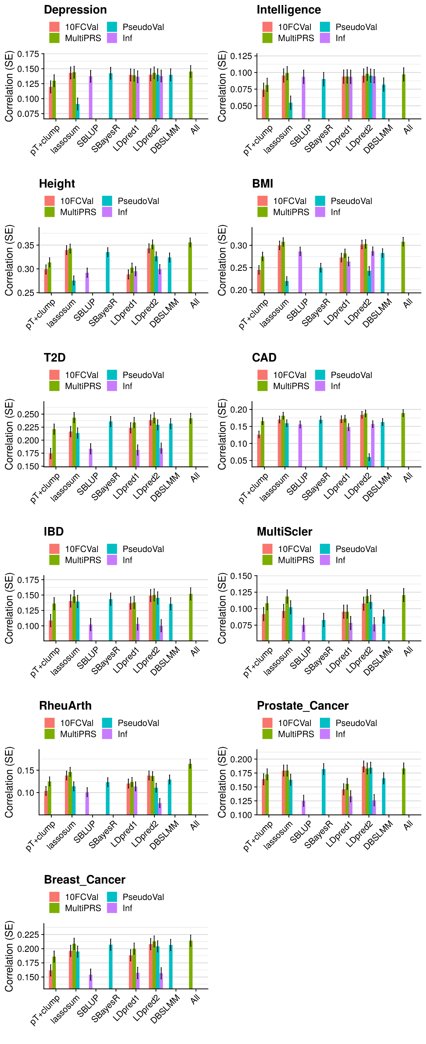
The performance for each polygenic scoring method across phenotypes was assessed using the correlation between observed and fitted values (Fig 2A), and then comparing each method with a baseline method of pT+clump with 10-fold cross validation using the difference in correlation (Fig 2B). All methods performed at least as well as pT+clump. These overview results show that the pseudovalidation (PseudoVal) and infinitesimal models (Inf) performed less well than polygenic scores selected through 10-fold cross-validation (10FCVal), and that the prediction when modelling multiple PRS (multi-PRS) was slightly higher than the 10-fold cross-validation. Full results for all traits in UKB and TEDS indicate consistency across methods, with no trait performing unexpectedly well or poorly on any single method (S6–S9 Tables; S4–S7 Figs).

Fig 2 — A) Average test-set correlation between predicted and observed values across phenotypes. B) Average difference between observed-prediction correlations for the best pT+clump polygenic score and all other methods. The average difference across phenotypes are shown as diamonds and the difference for each phenotype shown as transparent circles. Shows only results based on the UKB target sample when using the 1KG reference. Error bars indicate standard error of correlations for each method. 10FCVal represents a single polygenic score based on the optimal parameter as identified using 10-fold cross-validation. Multi-PRS represents an elastic net model containing polygenic scores based on a range of parameters, with elastic net shrinkage parameters derived using 10-fold cross-validation. PseudoVal represents a single polygenic score based on the predicted optimal parameter as identified using pseudovalidation, which requires no tuning sample. Inf represents a single polygenic score based on the infinitesimal model, which requires no tuning sample.

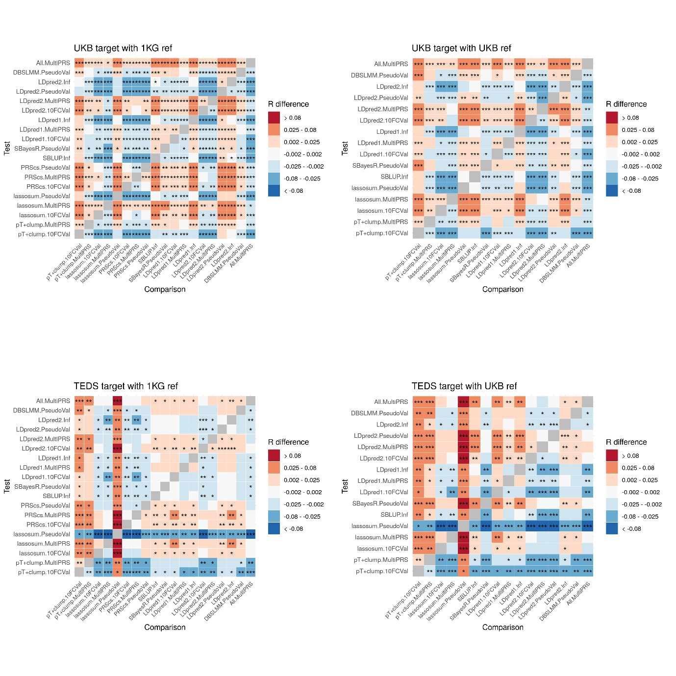
Comparison of polygenic scoring methods

A pairwise comparison of polygenic scoring methods was performed for each method (pT+clump, lassosum, PRScs, SBLUP, SBayesR, LDpred1, LDpred2, DBSLMM, All) and each model (10-fold cross validation, multi-PRS, pseudovalidation and infinitesimal). Fig 3 shows the difference in correlation (R) within and between methods for UKB outcomes with 1KG reference panel, with p-values for significant differences calculated using the William’s test results aggregated across outcomes. Full results for TEDS and UKB, and for both reference panels are given in S10–S13 Tables and S8 Fig, and by trait in S14–S17 Tables.

Fig 3 — Correlation difference = Test correlation–Comparison correlation. Red/orange coloring indicates the Test method (shown on Y axis) performed better than the Comparison method (shown on X axis). Shows only results based on the UKB target sample when using the 1KG reference. * = p<0.05. ** = p<1×10⁻³. *** = p<1×10⁻⁶. P-values are two-sided. 10FCVal represents a single polygenic score based on the optimal parameter as identified using 10-fold cross-validation. Multi-PRS represents an elastic net model containing polygenic scores based on a range of parameters, with elastic net shrinkage parameters derived using 10-fold cross-validation. PseudoVal represents a single polygenic score based on the predicted optimal parameter as identified using pseudovalidation, which requires no tuning sample. Inf represents a single polygenic score based on the infinitesimal model, which requires no tuning sample.

When using 10-fold cross validation to identify the optimal parameter, LDpred2, lassosum and PRScs provided the most predictive polygenic scores in the test sample on average, with a 16–18% relative improvement (p<8×10⁻¹⁶) over the 10-fold cross-validated pT+clump approach. When using 10-fold cross validation, on average LDpred2 provided a small but nominally significantly improved prediction over lassosum and PRScs (2%, p = 0.05).

Pseudovalidation and infinitesimal models do not require a tuning sample and their results are therefore described in parallel. The methods providing a pseudovalidation and/or infinitesimal approach include lassosum, PRScs, LDpred, LDpred2, SBLUP, DBSLMM and SBayesR. When using the smaller 1KG reference panel PRScs and DBSLMM performed the best on average, providing at least a 5% relative improvement (p<2×10⁻²) over other pseudovalidation approaches. The PRScs pseudovalidation approach provided a further significant improvement over DBSLMM, with an average relative improvement of 4% (p = 4×10⁻⁴). Furthermore, the PRScs pseudovalidation approach was on average only 3% (p-value = 6×10⁻³) worse than the best polygenic score identified by 10-fold cross validation for any method. When using the larger UKB reference panel, the performance of SBayesR improved and was not significantly different to that of DBSLMM. The performance of lassosum pseudovalidation, the LDpred1 and LDpred2 infinitesimal models, SBLUP, LDpred2 pseudovalidation and SBayesR was variable across phenotypes, whereas the PRScs pseudovalidated polygenic score achieved near optimal predication compared to any method, and always performed better than the best pT+clump polygenic scores as identified by 10-fold cross validation. The performances of DBSLMM, and SBayesR when using the larger UKB reference were also relatively stable across phenotypes.

Modelling multiple polygenic scores based on multiple parameters using an elastic net consistently outperformed models containing the single best polygenic score as identified using 10-fold cross validation. The improvement was largest when using pT+clump polygenic scores (12% relative improvement, p = 1×10⁻²¹), but was also statistically significant for lassosum (6% relative improvement, 3×10⁻¹⁵), PRScs (2% relative improvement, p = 4×10⁻⁵), LDpred1 (2% relative improvement, p = 4×10⁻⁵) and LDpred2 (2% relative improvement, p = 3×10⁻⁴ methods. On average, the ‘All’ method, combining polygenic scores across polygenic scoring methods provided a statistically significant improvement over the single best method (multi-PRS lassosum, 2% relative improvement, p = 4x10⁻³). Elastic net models using non-nested or dense p-value thresholds showed no improvement over the standard p-value thresholding approach (S18 and S19 Tables).

Convergence issues occurred for SBayesR for 4 of the 14 GWAS. In the latest version of the software implementing SBayesR (GCTB v2.03), developers have included a robust parameterization option which is automatically turned on when convergence issues are detected. We found that the robust parameterization resolved convergence issues, although the software had limited ability to detect convergence issues (S9 and S10 Figs). As a result, we recommend specifying the ‘--robust’ option to force the robust parameterization, as this optimized SBayesR performance in most instances (S9 and S10 Figs). Results comparing SBayesR to other methods reported in this study were derived using the robust parameterization option.

The relative performance of all methods and modelling approaches was similar across low and high polygenicity phenotypes (S11 Fig). Infinitesimal model-based polygenic scores performed better for high polygenicity phenotypes. Estimates of polygenicity for each phenotype are shown in S20 Table.

Controlling for the first 20 genetic principal components did not affect the relative performance of polygenic scoring methods (S12 Fig).

Runtime comparison

The runtime of methods to process GWAS summary statistics on chromosome 22 without parallel implementations varied substantially (S13 Fig). The methods (fastest to slowest) were pt+clump (~3 seconds), DBSLMM and lassosum (~30 seconds), SBLUP (~1 minute), SBayesR and LDpred1 (~3–6 minutes), PRScs (~35 minutes), and LDpred2 (~50 minutes). The number of parameters tested by each method will influence the runtime. For example, using only one shrinkage parameter for PRScs will take 1/5 of time taken for PRScs to use 5 shrinkage parameters.

Discussion

This study evaluated a range of polygenic scoring methods across phenotypes representing a range of genetic architectures and using reference and target sample genotypic data of different sample sizes. This study shows that, when a tuning sample is available to identify optimal parameters, more recently developed methods that do not perform LD-based clumping provide better prediction, with LDpred2, lassosum and PRScs providing a relative improvement of 16–18% compared to the pT+clump approach. When a tuning sample is not available, the optimal method for prediction was PRScs, with DBSLMM and SBayesR also performing well. Furthermore, the PRScs pseudovalidation performance was only 3% worse than the best polygenic scores identified by 10-fold cross validation for any other method. This study also shows that an elastic net model containing multiple polygenic scores based on a range of p-value thresholds or shrinkage parameters provides better prediction than the single best polygenic score as identified by 10-fold cross validation. Modelling multiple parameters increased prediction by 12% when using the pT+clump approach and 2–6% for polygenic scoring methods that model LD. Modelling polygenic scores from multiple methods provided a relative improvement of 1.7% in prediction over the single best method, though the additional computation time to perform all methods is substantial.

Our study highlighted the performance of SBayesR using default settings is highly variable across GWAS summary statistics due to convergence issues. However, convergence issues are avoided when the newly implemented robust parameterization option is specified.

These methods were evaluated within a reference-standardized framework and the results are likely to be generalizable to a range of settings, including a clinical setting. The improved transferability of prediction accuracy when using a reference-standardized approach enables prediction with a known accuracy for a single individual. This is an essential feature of any predictor as then its prediction can be appropriately considered in relation to other information about the individual. It is important to consider whether the reference-standardized approach impacts the predictive utility of the polygenic scores compared to those derived using target sample specific properties. The use of only HapMap3 variants is common for polygenic scoring methods as denser sets of variants increase the computational burden of the analysis and provide only incremental improvements in prediction [12]. However, denser sets of variants are ultimately likely to be of importance for optimizing the predictive utility of polygenic scores. The use of reference LD estimates instead of target sample-specific LD estimates is less likely to impact the predictive utility of polygenic scores. LD estimates are used to recapitulate LD structure in the GWAS discovery sample, and there should therefore be no advantage to using target sample specific LD estimates instead of reference sample LD estimates, unless the target sample better captures the LD structure in the GWAS discovery sample.

One major limitation of our study is that it was performed only in studies of European ancestry since GWAS of other ancestries have insufficient power for polygenic prediction. Polygenic scoring method comparisons in other ancestries or across ancestries will require substantial progress in diversifying genetic studies to non-European ancestry. In particular, it will be important to assess the impact of greater genetic diversity and weaker linkage disequilibrium in African ancestry populations. These studies are essential if polygenic risk scores are to be implemented in clinical care, to ensure equity of healthcare.

The clinical implementation of polygenic scores is at an early stage, and we identify five areas that still require further research. First, this study demonstrates that the reference-standardized approach provides reliable polygenic score estimates. However, the extent to which missing genetic variation within target sample data affects the prediction accuracy needs to be investigated. Furthermore, the extent to which prediction accuracy varies across individuals from different European ancestral populations needs to be assessed. Second, this study used the HapMap3 SNP list when deriving polygenic scores, building on previous research suggesting that these variants are reliably imputed and provide good coverage of the genome [20]. However, other sets of variants should be explored as denser coverage of the genome may improve prediction. Third, this study investigates polygenic scores based on a single discovery GWAS or phenotype. Previous research has shown that methods which combine evidence across multiple GWAS can improve prediction due to genetic correlation between traits [37–41]. Further research comparing the predictive utility of multi-trait polygenic prediction within a reference-standardized framework is required. Fourth, we present the reference standardized approach as a conceptual framework for implementing polygenic scores in a clinical setting. However, several additional issues will need to be addressed before they can be used in a clinical setting, such as assigning individuals to the optimal reference population, the presence of admixture, and translating relative polygenic scores into absolute terms. Finally, integration of functional genomic annotations has been shown to improve prediction over functionally agnostic polygenic scoring methods [42]. Comparison of functionally informed methods within a reference-standardized framework is also required.

In conclusion, this study performed a comprehensive comparison of GWAS summary statistic-based polygenic scoring methods within a reference-standardized framework using European ancestry studies. The results provide a useful resource for future research and endeavors to implement polygenic scores for individual-level prediction. All the code, rationale and results of this study are available on the GenoPred website (see Web Resources). This website will continue to document the evaluation of novel genotype-based prediction methods, providing a valuable community resource for education, research, and collaboration. Novel polygenic score methods can be rapidly tested against these standard methods to benchmark performance. This framework should be a valuable tool in the roadmap of moving polygenic risk scores from research studies to clinical implementation. Further investigation of methods providing genotype-based prediction within a reference-standardized framework is needed.

Supporting information

S1 Fig. Schematic diagram showing UKB was split into reference, training and testing samples.

A sample of UKB providing 50,000 observations for each phenotype was identified. The sample was then further split into training (80%) and testing (20%) samples. The training sample used 10-fold cross validation to identify the optimal polygenic scoring parameters and elastic net hyper-parameters. An independent sample of 10,000 European UKB participants was also created to as a reference for polygenic scoring.

(PNG)

Click here for additional data file.^{(95.2KB, png)}

S2 Fig. Average test-set correlation between predicted and observed values across phenotypes.

Error bars indicate standard error of correlations for each method. Results are split by the target and reference genotypic data used. Results are 10FCVal bars represent a single polygenic score based on the optimal parameter as identified using 10-fold cross-validation. Multi-PRS bars represent an elastic net model containing polygenic scores based on a range of parameters, with elastic net shrinkage parameters derived using 10-fold cross-validation. PseudoVal bars represent a single polygenic score based on the predicted optimal parameter as identified using pseudovalidation, which requires no tuning sample. Inf represents a single polygenic score based on the infinitesimal model, which requires no tuning sample.

(PNG)

Click here for additional data file.^{(152.2KB, png)}

S3 Fig. Average test-set observed-expected correlation difference between the best pT+clump polygenic score and all other methods.

The average difference across phenotypes are shown as diamonds with error bars indicating the standard error, and the difference for each phenotype shown as transparent circles. Results are split by the target and reference genotypic data used. 10FCVal represents a single polygenic score based on the optimal parameter as identified using 10-fold cross-validation. Multi-PRS represents an elastic net model containing polygenic scores based on a range of parameters, with elastic net shrinkage parameters derived using 10-fold cross-validation. PseudoVal represents a single polygenic score based on the predicted optimal parameter as identified using pseudovalidation, which requires no tuning sample. Inf represents a single polygenic score based on the infinitesimal model, which requires no tuning sample.

(PNG)

Click here for additional data file.^{(198.6KB, png)}

S4 Fig. Correlation between predicted and observed values for each phenotype in UKB when using the European subset of 1000 Genomes as the reference.

Error bars indicate standard errors. 10FCVal bars represent a single polygenic score based on the optimal parameter as identified using 10-fold cross-validation. Multi-PRS bars represent an elastic net model containing polygenic scores based on a range of parameters, with elastic net shrinkage parameters derived using 10-fold cross-validation. PseudoVal bars represent a single polygenic score based on the predicted optimal parameter as identified using pseudovalidation, which requires no tuning sample. Inf represents a single polygenic score based on the infinitesimal model, which requires no tuning sample.

(PNG)

Click here for additional data file.^{(548.5KB, png)}

S5 Fig. Correlation between predicted and observed values for each phenotype in UKB when using an independent 10K subset of European UKB individuals as the reference.

(PNG)

Click here for additional data file.^{(520KB, png)}

S6 Fig. Correlation between predicted and observed values for each phenotype in TEDS when using the European subset of 1000 Genomes as the reference.

Error bars indicate standard errors. 10FCVal bars represent a single polygenic score based on the optimal parameter as identified using 10-fold cross-validation. Multi-PRS bars represent an elastic net model containing polygenic scores based on a range of parameters, with elastic net shrinkage parameters derived using 10-fold cross-validation. PseudoVal bars represent a single polygenic score based on the predicted optimal parameter as identified using pseudovalidation, which requires no tuning sample.1000G Reference. Inf represents a single polygenic score based on the infinitesimal model, which requires no tuning sample.

(PNG)

Click here for additional data file.^{(204.5KB, png)}

S7 Fig. Correlation between predicted and observed values for each phenotype in TEDS when using an independent 10K subset of European UKB individuals as the reference.

(PNG)

Click here for additional data file.^{(191KB, png)}

S8 Fig. Average test-set observed-expected correlation difference between all methods with significance value.

Correlation difference = Test correlation–Reference correlation. Shows only results based on the UKB target sample when using the 1KG reference as other results were highly concordant. * = p<0.05. ** = p<1×10⁻³. *** = p<1×10⁻⁶. P-values are one-sided. 10FCVal corresponds to a single polygenic score based on the optimal parameter as identified using 10-fold cross-validation. Multi-PRS corresponds to an elastic net model containing polygenic scores based on a range of parameters, with elastic net shrinkage parameters derived using 10-fold cross-validation. PseudoVal corresponds to a single polygenic score based on the predicted optimal parameter as identified using pseudovalidation, which requires no tuning sample. Inf represents a single polygenic score based on the infinitesimal model, which requires no tuning sample.

(PNG)

Click here for additional data file.^{(368.6KB, png)}

S9 Fig. Correlation between predicted and observed values across phenotypes in UKB for SBayesR polygenic scores derived using different reference samples and different GWAS processing procedures.

1KG indicates the reference sample was the European subset of 1000 Genomes. UKB indicates the reference sample was an independent 10K subset of European UKB individuals. GCTB indicates the reference was the GCTB-provided reference data based on a non-independent 50K subset of European UKB individuals. The colour of the bars indicates the version of GCTB used when running SBayesR and which settings were used. Default indicates that default settings were used. P<0.4 indicates only variants with a GWAS p-value <0.4 were retained. Robust indicates that the—robust parameter was specified, forcing robust parameterisation.

(PNG)

Click here for additional data file.^{(195.8KB, png)}

S10 Fig. Correlation between predicted and observed values across phenotypes in TEDS for SBayesR polygenic scores derived using different reference samples and different GWAS processing procedures.

(PNG)

Click here for additional data file.^{(177.3KB, png)}

S11 Fig. Comparison of methods across high and low polygenicity outcomes in UKB target sample using 1KG reference.

Figure shows average test-set observed-expected correlation difference between the best pT+clump polygenic score and all other methods. The average difference across phenotypes are shown as diamonds with error bars indicating the standard error, and the difference for each phenotype shown as transparent circles. 10FCVal represents a single polygenic score based on the optimal parameter as identified using 10-fold cross-validation. Multi-PRS represents an elastic net model containing polygenic scores based on a range of parameters, with elastic net shrinkage parameters derived using 10-fold cross-validation. PseudoVal represents a single polygenic score based on the predicted optimal parameter as identified using pseudovalidation, which requires no tuning sample. Inf represents a single polygenic score based on the infinitesimal model, which requires no tuning sample.

(PNG)

Click here for additional data file.^{(88.2KB, png)}

S12 Fig. Comparison of methods after controlling for genetic principal components in UKB target sample using 1KG reference.

(PNG)

Click here for additional data file.^{(94.4KB, png)}

S13 Fig. Runtime for each polygenic scoring method using genetic variants on chromosome 22.

No parallel implementations were used.

(PNG)

Click here for additional data file.^{(32.7KB, png)}

S1 Table. Descriptive statistics for GWAS summary statistics used to predict target sample phenotypes.

(XLSX)

Click here for additional data file.^{(12.5KB, xlsx)}

S2 Table. Average performance in UKB with 1KG reference.

(XLSX)

Click here for additional data file.^{(11.1KB, xlsx)}

S3 Table. Average performance in UKB with UKB reference.

(XLSX)

Click here for additional data file.^{(10KB, xlsx)}

S4 Table. Average performance in TEDS with 1KG reference.

(XLSX)

Click here for additional data file.^{(10.1KB, xlsx)}

S5 Table. Average performance in TEDS with UKB reference.

(XLSX)

Click here for additional data file.^{(10KB, xlsx)}

S6 Table. Polygenic prediction in UKB using EUR 1KG reference.

(XLSX)

Click here for additional data file.^{(38.2KB, xlsx)}

S7 Table. Polygenic prediction in UKB using EUR 10K UKB reference.

(XLSX)

Click here for additional data file.^{(31.7KB, xlsx)}

S8 Table. Polygenic prediction in TEDS using EUR 1KG reference.

(XLSX)

Click here for additional data file.^{(15.5KB, xlsx)}

S9 Table. Polygenic prediction in TEDS using EUR 10K UKB reference.

(XLSX)

Click here for additional data file.^{(13.8KB, xlsx)}

S10 Table. Average difference between methods in UKB with 1KG reference.

(XLSX)

Click here for additional data file.^{(38.7KB, xlsx)}

S11 Table. Average difference between methods in UKB with UKB reference.

(XLSX)

Click here for additional data file.^{(29.2KB, xlsx)}

S12 Table. Average difference between methods in TEDS with 1KG reference.

(XLSX)

Click here for additional data file.^{(36.7KB, xlsx)}

S13 Table. Average difference between methods in TEDS with UKB reference.

(XLSX)

Click here for additional data file.^{(29KB, xlsx)}

S14 Table. Difference between methods in UKB with 1KG reference.

(XLSX)

Click here for additional data file.^{(275.4KB, xlsx)}

S15 Table. Difference between methods in UKB with UKB reference.

(XLSX)

Click here for additional data file.^{(195.7KB, xlsx)}

S16 Table. Difference between methods in TEDS with 1KG reference.

(XLSX)

Click here for additional data file.^{(104.5KB, xlsx)}

S17 Table. Difference between methods in TEDS with UKB reference.

(XLSX)

Click here for additional data file.^{(75.6KB, xlsx)}

S18 Table. Correlation between pT+clump model predictions and observed values in UK Biobank.

(XLSX)

Click here for additional data file.^{(11.6KB, xlsx)}

S19 Table. Correlation between pT+clump model predictions and observed values in TEDS.

(XLSX)

Click here for additional data file.^{(10.3KB, xlsx)}

S20 Table. AVENGEME Estimates of Polygenicity.

(XLSX)

Click here for additional data file.^{(18KB, xlsx)}

S1 Supplementary Text. Provides description of outcome definitions in UKB and TEDS, methodology for estimating polygenicity, and SBayesR sensitivity analyses.

(DOCX)

Click here for additional data file.^{(25.5KB, docx)}

Acknowledgments

We thank Luke Lloyd-Jones and Jian Zeng for their advice on SBayesR using GCTB, Tian Ge on using PRScs, and Florian Privé on using LDpred2. We thank Paul O’Reilly and Sam Choi for useful discussion.

The authors acknowledge use of the research computing facility at King’s College London, Rosalind (https://rosalind.kcl.ac.uk), which is delivered in partnership with the NIHR Maudsley BRC, and part-funded by capital equipment grants from the Maudsley Charity (award 980) and Guy’s & St. Thomas’ Charity (TR130505). The views expressed are those of the authors and not necessarily those of the NHS, the NIHR or the Department of Health and Social Care. We thank the research participants and employees of 23andMe for making the work regarding Depression possible.

UKB: This research was conducted under UK Biobank application 18177.

TEDS: We gratefully acknowledge the ongoing contribution of the participants in TEDS and their families. TEDS is supported by UK Medical Research Council Program Grant MR/M021475/1 (and previously Grant G0901245) (to Robert Plomin (R.P).), with additional support from National Institutes of Health Grant AG046938. The research leading to these results has also received funding from the European Research Council under the European Union’s Seventh Framework Programme (FP7/2007-2013) ERC Grant Agreement 295366. R.P. is supported by Medical Research Council Research Professor Award G19/2. KR is supported by a Sir Henry Wellcome Postdoctoral Fellowship (213514/Z/18/Z).

Web resources

LDSC HapMap 3 SNP-list: https://data.broadinstitute.org/alkesgroup/LDSCORE/w_hm3.snplist.bz2
LDSC Munge Sumstats: https://github.com/bulik/ldsc/blob/master/munge_sumstats.py
GCTB LD matrices: https://zenodo.org/record/3350914
Impute.me: https://impute.me/
GenoPred: https://opain.github.io/GenoPred

Data Availability

A data transfer agreement is required to access individual-level data for TEDS (https://www.teds.ac.uk/researchers/teds-data-access-policy) and UK Biobank(https://biobank.ctsu.ox.ac.uk/crystal/exinfo.cgi?src=accessing_data_guide). The code used during this study are available at GitHub: https://opain.github.io/GenoPred.

Funding Statement

This study was funded by the UK Medical Research Council (https://mrc.ukri.org/): MR/N015746/1 to CML and MR/S0151132 to SH. CML was also funded by the National Institute for Health Research (NIHR) Biomedical Research Centre at South London and Maudsley NHS Foundation Trust and King’s College London (https://www.maudsleybrc.nihr.ac.uk/). The funders had no role in study design, data collection and analysis, decision to publish, or preparation of the manuscript.

References

1.Polderman TJC, Benyamin B, de Leeuw CA, Sullivan PF, van Bochoven A, Visscher PM, et al. Meta-analysis of the heritability of human traits based on fifty years of twin studies. Nat Genet. 2015;47: 702–9. 10.1038/ng.3285 [DOI] [PubMed] [Google Scholar]
2.Manolio TA, Collins FS, Cox NJ, Goldstein DB, Hindorff LA, Hunter DJ, et al. Finding the missing heritability of complex diseases. Nature. 2009;461: 747–753. 10.1038/nature08494 [DOI] [PMC free article] [PubMed] [Google Scholar]
3.Buniello A, MacArthur JAL, Cerezo M, Harris LW, Hayhurst J, Malangone C, et al. The NHGRI-EBI GWAS Catalog of published genome-wide association studies, targeted arrays and summary statistics 2019. Nucleic Acids Res. 2019;47: D1005–D1012. 10.1093/nar/gky1120 [DOI] [PMC free article] [PubMed] [Google Scholar]
4.Consortium IS. Common polygenic variation contributes to risk of schizophrenia and bipolar disorder. Nature. 2009;460: 748. 10.1038/nature08185 [DOI] [PMC free article] [PubMed] [Google Scholar]
5.Dudbridge F. Power and Predictive Accuracy of Polygenic Risk Scores. PLoS Genet. 2013;9. 10.1371/journal.pgen.1003348 [DOI] [PMC free article] [PubMed] [Google Scholar]
6.Choi SW, Mak TSH, O’reilly P. A guide to performing Polygenic Risk Score analyses. BioRxiv. 2018; 416545. [DOI] [PMC free article] [PubMed] [Google Scholar]
7.Choi SW, O’Reilly PF. PRSice-2: Polygenic Risk Score software for biobank-scale data. Gigascience. 2019;8: giz082. 10.1093/gigascience/giz082 [DOI] [PMC free article] [PubMed] [Google Scholar]
8.Vilhjálmsson BJ, Yang J, Finucane HK, Gusev A, Lindström S, Ripke S, et al. Modeling linkage disequilibrium increases accuracy of polygenic risk scores. Am J Hum Genet. 2015;97: 576–592. 10.1016/j.ajhg.2015.09.001 [DOI] [PMC free article] [PubMed] [Google Scholar]
9.Robinson MR, Kleinman A, Graff M, Vinkhuyzen AAE, Couper D, Miller MB, et al. Genetic evidence of assortative mating in humans. Nat Hum Behav. 2017;1: 16. [Google Scholar]
10.Mak TSH, Porsch RM, Choi SW, Zhou X, Sham PC. Polygenic scores via penalized regression on summary statistics. Genet Epidemiol. 2017;41: 469–480. 10.1002/gepi.22050 [DOI] [PubMed] [Google Scholar]
11.Ge T, Chen C-Y, Ni Y, Feng Y-CA, Smoller JW. Polygenic prediction via Bayesian regression and continuous shrinkage priors. Nat Commun. 2019;10: 1–10. 10.1038/s41467-018-07882-8 [DOI] [PMC free article] [PubMed] [Google Scholar]
12.Lloyd-Jones LR, Zeng J, Sidorenko J, Yengo L, Moser G, Kemper KE, et al. Improved polygenic prediction by Bayesian multiple regression on summary statistics. Nat Commun. 2019;10: 1–11. 10.1038/s41467-018-07882-8 [DOI] [PMC free article] [PubMed] [Google Scholar]
13.Privé F, Arbel J, Vilhjálmsson BJ. LDpred2: better, faster, stronger. Bioinformatics. 2020. 10.1093/bioinformatics/btaa1029 [DOI] [PMC free article] [PubMed] [Google Scholar]
14.Yang S, Zhou X. Accurate and scalable construction of polygenic scores in large biobank data sets. Am J Hum Genet. 2020;106: 679–693. 10.1016/j.ajhg.2020.03.013 [DOI] [PMC free article] [PubMed] [Google Scholar]
15.Allegrini AG, Selzam S, Rimfeld K, von Stumm S, Pingault J-B, Plomin R. Genomic prediction of cognitive traits in childhood and adolescence. Mol Psychiatry. 2019;24: 819–827. 10.1038/s41380-019-0394-4 [DOI] [PMC free article] [PubMed] [Google Scholar]
16.Ni G, Zeng J, Revez JR, Wang Y, Ge T, Restaudi R, et al. A comprehensive evaluation of polygenic score methods across cohorts in psychiatric disorders. MedRxiv. 2020. [Google Scholar]
17.Coombes BJ, Biernacka JM. A principal component approach to improve association testing with polygenic risk scores. BioRxiv. 2019; 847020. [DOI] [PMC free article] [PubMed] [Google Scholar]
18.Privé F, Vilhjálmsson BJ, Aschard H, Blum MGB. Making the most of Clumping and Thresholding for polygenic scores. Am J Hum Genet. 2019;105: 1213–1221. 10.1016/j.ajhg.2019.11.001 [DOI] [PMC free article] [PubMed] [Google Scholar]
19.Lewis CM, Vassos E. Polygenic risk scores: from research tools to clinical instruments. Genome Med. 2020;12: 1–11. 10.1186/s13073-020-00742-5 [DOI] [PMC free article] [PubMed] [Google Scholar]
20.International HapMap 3 Consortium, investigators P, leaders P coordination, group M writing, QC G, and discovery E 3 sequencing, et al. Integrating common and rare genetic variation in diverse human populations. Nature. 2010;467: 52–58. 10.1038/nature09298 [DOI] [PMC free article] [PubMed] [Google Scholar]
21.Consortium 1000 Genomes Project. A global reference for human genetic variation. Nature. 2015;526: 68–74. 10.1038/nature15393 [DOI] [PMC free article] [PubMed] [Google Scholar]
22.Folkersen L, Pain O, Ingason A, Werge T, Lewis CM, Austin J. Impute. me: an open source, non-profit tool for using data from DTC genetic testing to calculate and interpret polygenic risk scores. BioRxiv. 2019; 861831. [DOI] [PMC free article] [PubMed] [Google Scholar]
23.Bycroft C, Freeman C, Petkova D, Band G, Elliott LT, Sharp K, et al. The UK Biobank resource with deep phenotyping and genomic data. Nature. 2018;562: 203–209. 10.1038/s41586-018-0579-z [DOI] [PMC free article] [PubMed] [Google Scholar]
24.Rimfeld K, Malanchini M, Spargo T, Spickernell G, Selzam S, McMillan A, et al. Twins early development study: A genetically sensitive investigation into behavioral and cognitive development from infancy to emerging adulthood. Twin Res Hum Genet. 2019; 1–6. 10.1017/thg.2018.75 [DOI] [PMC free article] [PubMed] [Google Scholar]
25.McCarthy S, Das S, Kretzschmar W, Delaneau O, Wood AR, Teumer A, et al. A reference panel of 64,976 haplotypes for genotype imputation. Nat Genet. 2016. 10.1038/ng.3643 [DOI] [PMC free article] [PubMed] [Google Scholar]
26.consortium U. The UK10K project identifies rare variants in health and disease. Nature. 2015;526: 82–90. 10.1038/nature14962 [DOI] [PMC free article] [PubMed] [Google Scholar]
27.Glanville KP, Coleman JRI, Hanscombe KB, Euesden J, Choi SW, Purves KL, et al. Classical human leukocyte antigen alleles and C4 haplotypes are not significantly associated with depression. Biol Psychiatry. 2020;87: 419–430. 10.1016/j.biopsych.2019.06.031 [DOI] [PMC free article] [PubMed] [Google Scholar]
28.Selzam S, McAdams TA, Coleman JRI, Carnell S, O’Reilly PF, Plomin R, et al. Evidence for gene-environment correlation in child feeding: Links between common genetic variation for BMI in children and parental feeding practices. PLoS Genet. 2018;14. 10.1371/journal.pgen.1007757 [DOI] [PMC free article] [PubMed] [Google Scholar]
29.Selzam S, Ritchie SJ, Pingault J-B, Reynolds CA, O’Reilly PF, Plomin R. Comparing within-and between-family polygenic score prediction. Am J Hum Genet. 2019;105: 351–363. 10.1016/j.ajhg.2019.06.006 [DOI] [PMC free article] [PubMed] [Google Scholar]
30.Chang CC, Chow CC, Tellier LCAM, Vattikuti S, Purcell, Lee JJ. Second-generation PLINK: rising to the challenge of larger and richer datasets. Gigascience. 2015;4: 1. 10.1186/s13742-015-0047-8 [DOI] [PMC free article] [PubMed] [Google Scholar]
31.Zeng J, De Vlaming R, Wu Y, Robinson MR, Lloyd-Jones LR, Yengo L, et al. Signatures of negative selection in the genetic architecture of human complex traits. Nat Genet. 2018;50: 746. 10.1038/s41588-018-0101-4 [DOI] [PubMed] [Google Scholar]
32.Lee SH, Goddard ME, Wray NR, Visscher PM. A better coefficient of determination for genetic profile analysis. Genet Epidemiol. 2012;36: 214–224. 10.1002/gepi.21614 [DOI] [PubMed] [Google Scholar]
33.Zou H, Hastie T. Regularization and variable selection via the elastic net. J R Stat Soc Ser B (statistical Methodol. 2005;67: 301–320. [Google Scholar]
34.Steiger JH. Tests for comparing elements of a correlation matrix. Psychol Bull. 1980;87: 245. [Google Scholar]
35.Cooper H, Hedges LV, Valentine JC. The handbook of research synthesis and meta-analysis 2nd edition. The Hand of Res Synthesis and Meta-Analysis, 2nd Ed. Russell Sage Foundation; 2009. pp. 1–615. [Google Scholar]
36.Palla L, Dudbridge F. A fast method that uses polygenic scores to estimate the variance explained by genome-wide marker panels and the proportion of variants affecting a trait. Am J Hum Genet. 2015;97: 250–259. 10.1016/j.ajhg.2015.06.005 [DOI] [PMC free article] [PubMed] [Google Scholar]
37.Krapohl E, Patel H, Newhouse S, Curtis CJ, von Stumm S, Dale PS, et al. Multi-polygenic score approach to trait prediction. Mol Psychiatry. 2018;23: 1368–1374. 10.1038/mp.2017.163 [DOI] [PMC free article] [PubMed] [Google Scholar]
38.Grotzinger AD, Rhemtulla M, de Vlaming R, Ritchie SJ, Mallard TT, Hill WD, et al. Genomic structural equation modelling provides insights into the multivariate genetic architecture of complex traits. Nat Hum Behav. 2019;3: 513–525. 10.1038/s41562-019-0566-x [DOI] [PMC free article] [PubMed] [Google Scholar]
39.Maier RM, Zhu Z, Lee SH, Trzaskowski M, Ruderfer DM, Stahl EA, et al. Improving genetic prediction by leveraging genetic correlations among human diseases and traits. Nat Commun. 2018;9: 1–17. 10.1038/s41467-017-02088-w [DOI] [PMC free article] [PubMed] [Google Scholar]
40.Turley P, Walters RK, Maghzian O, Okbay A, Lee JJ, Fontana MA, et al. Multi-trait analysis of genome-wide association summary statistics using MTAG. Nat Genet. 2018;50: 229–237. 10.1038/s41588-017-0009-4 [DOI] [PMC free article] [PubMed] [Google Scholar]
41.Inouye M, Abraham G, Nelson CP, Wood AM, Sweeting MJ, Dudbridge F, et al. Genomic risk prediction of coronary artery disease in 480,000 adults: implications for primary prevention. J Am Coll Cardiol. 2018;72: 1883–1893. 10.1016/j.jacc.2018.07.079 [DOI] [PMC free article] [PubMed] [Google Scholar]
42.Marquez-Luna C, Gazal S, Loh P-R, Furlotte N, Auton A, Price AL, et al. Modeling functional enrichment improves polygenic prediction accuracy in UK Biobank and 23andMe data sets. bioRxiv. 2018; 375337. [DOI] [PMC free article] [PubMed] [Google Scholar]

PLoS Genet. doi: 10.1371/journal.pgen.1009021.r001

Decision Letter 0

David Balding, Vincent Plagnol

25 Oct 2020

Dear Dr Pain,

Thank you very much for submitting your Research Article entitled 'Evaluation of Polygenic Prediction Methodology within a Reference-Standardized Framework' to PLOS Genetics. Your manuscript was fully evaluated at the editorial level and by independent peer reviewers. As you can see, the three reviewers engaged constructively with the paper and made good comments. Based on these reviews, we would welcome a revised version of the manuscript, while not being able to promise, of course, publication at that time.

Reading through the reviews, a specific comment that occurred to me before I sent this paper out for review and that was confirmed by reviewers is the need to report more standard metrics for binary outcomes (AUC/OR per SD). I mention this because one of my first reaction was to line up these results with my personal intuition, and while I appreciate your argument that a corresponding value can be estimated in theory, it remains a hurdle. So that would be a meaningful improvement.

A reviewer noted that not all existing methods are presented but that is understandable of course- there are simply too many. As an editor, I will not require that you extend a lot the set of methods included but please try to consider that comment if you can. On the other hand, a small number of additional disease traits (breast cancer for example?) would be helpful. The cancer space is of particular interest and should be highlighted.

More generally, the reviewers have made many suggestions for improvements and additional comparisons. We won't expect you to fully meet every such request but we would like to see some substantial improvements in a revised version - we leave to you to choose the most important additions that can be made to improve the manuscript within a reasonable time frame. Your response letter should address all the points made by each reviewer and justify the decisions that you made, as well as a description of the changes you have made in the manuscript.

If you decide to revise the manuscript for further consideration at PLOS Genetics, please aim to resubmit within the next 60 days, unless it will take extra time to address the concerns of the reviewers, in which case we would appreciate an expected resubmission date by email to plosgenetics@plos.org.

If present, accompanying reviewer attachments are included with this email; please notify the journal office if any appear to be missing. They will also be available for download from the link below. You can use this link to log into the system when you are ready to submit a revised version, having first consulted our Submission Checklist.

Please be aware that our data availability policy requires that all numerical data underlying graphs or summary statistics are included with the submission, and you will need to provide this upon resubmission if not already present. In addition, we do not permit the inclusion of phrases such as "data not shown" or "unpublished results" in manuscripts. All points should be backed up by data provided with the submission.

While revising your submission, please upload your figure files to the Preflight Analysis and Conversion Engine (PACE) digital diagnostic tool. PACE helps ensure that figures meet PLOS requirements. To use PACE, you must first register as a user. Then, login and navigate to the UPLOAD tab, where you will find detailed instructions on how to use the tool. If you encounter any issues or have any questions when using PACE, please email us at figures@plos.org.

PLOS has incorporated Similarity Check, powered by iThenticate, into its journal-wide submission system in order to screen submitted content for originality before publication. Each PLOS journal undertakes screening on a proportion of submitted articles. You will be contacted if needed following the screening process.

To resubmit, use the link below and 'Revise Submission' in the 'Submissions Needing Revision' folder.

[LINK]

We are sorry that we cannot be more positive about your manuscript at this stage. Please do not hesitate to contact us if you have any concerns or questions.

Yours sincerely,

Vincent Plagnol

Associate Editor

PLOS Genetics

David Balding

Section Editor: Methods

PLOS Genetics

Reviewer's Responses to Questions

Comments to the Authors:

Reviewer #1: In this report, Pain et al. set out to benchmark various polygenic score algorithms as well as two reference panels across a range of 13 traits. They determine that on average: (i) all scores outperformed pruning and thresholding based approaches; (ii) PRScs delivered performance comparable to other approaches but dit not require a tuning set; (iii) use of a polygenic score based on an elastic net tended to outperform other strategies.

I do think that this approach will be of interest to the general genetics community.

* Please clarify - multiPRS for each algorithms are based on combining multiple scores derived from a single algorithm?

* Can score performance be improved using an elastic net of scores using multiple different algorithms do even better?

* I think correlation is used as a surrogate for accuracy, but I wonder if additional metrics should also be reported (e.g. a measure of discrimination for binary phenotypes or OR/SD commonly used), can get ideas from the Wand et al. preprint one polygenic score reporting standards from ClinGen

* For P&T, what r2 value(s) were used?

* Can authors comment on general principle of being able to predict which approach might work the best based on heritability, polygenicity, etc.? e.g. autoimmune diseases have a very different architecture so could be optimized using a different approach.

* For lassosum, is it appropriate to have a set lambda (as opposed to letting the software choose one as done in glimnet R package)?

* I found Figure 3 quite confusing and nonintuitive, would encourage an alternate presentation style.

* Please clarify how scores will be shared with research community.

Reviewer #2: This manuscript sets out to compare several methods for deriving polygenic

scores, across 13 phenotypes, in the UK Biobank and TEDS study. Several tuning

strategies are compared (10-fold cross-validation, pseudovalidation). With the

large number of polygenic score methods today, it is useful for the human

genetics community to benchmark which approaches are more promising.

Overall, this manuscript is a timely and useful addition to the literature. At

the same time, there are many methods being compared across different phenotypes

and often I found it difficult to follow the logic of the analysis and what

message each key result was trying to convey. In addition, some of the key

concepts (e.g., what pseudovalidation means for each method) aren't explained,

making the results hard to understand, especially for readers who aren't

experts in PRS.

Major comments:

===============

* It's not clear whether the terminology of 'reference standardized approach'

narrowly refers to the use of the same LD reference panels and HapMap3 SNPs to

enable consistent evaluation of methods, or to a wider conceptual framework for

precision medicine; this really needs clarification. If it's only the former,

then it's simply good scientific practice to benchmark tools consistently and is

fine as is (with clarification). But if it's the latter (e.g., as hinted in

Discussion pg 22, line 453), then it should be acknowledged that this is only

the first step in such an endeavour and more complex issues will arise, e.g.,

matching the target sample to the best reference sample, admixture, absolute

risk and calibration, etc.

* What's the reasoning behind limiting the sample size to n=50,000 for all

phenotypes?

* Figure 1: What is the difference between the boxes 'Pre-imputed genotype data'

and 'Observed genome-wide genotype data'?

* An illustration of the actual study design (e.g., the split of UKB into

various reference/tuning/testing subsets etc, and sample sizes in each) would be

very useful as a supplementary figure, I found it difficult to follow which

dataset went into which analysis.

* Can you briefly explain pseudovalidation, and why you consider SBLUP/SBayesR

as methods that don't require cross-validation? LDpred has a single parameter

too, yet it was used in cross-validation.

* For the summary stats, is any MAF cutoff used, and are the same exact SNPs

used by all methods across all summary stats? e.g., LDpred v1 by default filters

out SNPs with MAF<1% and/or palindromic SNPs, but other methods may not.

* For the MultiPRS, it's not clear what kind of PRS went into it. Was it only

P+T based PRS or others as well? How many scores?

* Fig 2B, the caption and legend mention diamonds, but the actual figure shows

little stars, are they referring to the same thing?

* More of a comment / Discussion item, the cross-validation (including the

MultiPRS) will be affected by the number of cases in the training set, which is

quite small for some phenotypes in the UKB (e.g., multiple sclerosis), but isn't

really an inherent 'biological' feature of that disease/phenotype but more of a

UKB limitation.

* Figure 3: It's not clear what this figure is trying to convey. Does Reference

mean the n=10,000 UKB dataset? This should be explained in the figure or the

caption. Also the caption says 'For columns, red/orange coloring indicates the

Test method performed better than the Test method (horizontal)', do you mean

'performed better than the Reference method'?

Minor comments:

===============

* For the UK Biobank, does 'European ancestry' here mean the British White

subset or is it a wider definition?

* pg 15, line 312 'logistic regression was used...', it's not clear why this is

under the 'Estimating prediction accuracy' subsection, and how does it apply to

these PRS methods? Most of the PRS methods assume a linear regression model even

for binary outcomes.

* Which version of LDpred was used?

* pg 5, line 63: 'Although genetic information is used to predict rare Mendelian

genetic disorders' -> most of the time rare Mendelian genetic disorders don't

need prediction since they manifest early in life, are highly penetrant, and

testing usually occurs after clinical presentation and not before. Perhaps

BRCA1/2 is the one standout example you can use here.

* pg 6, line 98: 'Effect sizes estimated in a GWAS are typically larger than

they would be in an independent sample due to overfitting or winner’s curse'.

This text could use some clarification as it could confuse readers; in standard

GWAS, there is no overfitting (one predictor with thousands of samples) but due

to p-value selection there is a winner's curse which leads to inflation of

effect sizes for the statistically significant SNPs. In contrast, in

multivariable models (e.g., BLUP or lasso) there can be overfitting since the

number of SNPs is typically much larger than the sample size.

* It's quite confusing to call one result '10FCVal' and another 'MultiPRS' when

the MultiPRS also used 10-fold cross-validation.

* pg 24, line 497, much more salient examples of MultiPRS (aka metaGRS)

improving predictive power over single PRS are

https://www.onlinejacc.org/content/72/16

https://www.nature.com/articles/s41467-019-13848-1

* Table 2: It's not quite right to say that e.g., LDpred needs only 'direction

of effect' as variant level data. LDpred v1 uses the (two-sided) p-value to

back-calculate the unsigned z-statistic, and it needs the effect direction to be

able to infer the sign of the original (signed) z-statistic. So it basically

needs both beta and the p-value.

* Discussion, pg 23 'Then prediction is the aim and inference is not of

interest...': this paragraph is confusing. Adjusting PRS for PCs doesn't affect

whether prediction is the aim or not, but affects interpretation. If there is

substantial population stratification in the GWAS and/or target population that

is also correlated with the phenotype of interest, the analysis needs to be very

careful due to potential for confounding. Arguably, we don't want PRS for T2D

being good at prediction just because they predict people's ancestry which is

confounded with socioeconomic status. It does get rather blurry for phenotypes

like educational attainment.

Reviewer #3: Pain et al present a well written and a very timely benchmark study for polygenic risk score methods. In recent years a number of different methods have been proposed to derive polygenic risk scores based on GWAS summary statistics, and almost every paper finds that their proposed method is somehow the “best”. As a user, it is therefore hard to understand what method to use for a given dataset. Therefore benchmark studies like these are particularly timely and important. However, I feel that the benchmarks provided here do not necessarily provide a full picture of the field. First, not all published methods are considered in the benchmark, although some of the most commonly used are included. Second, only about a dozen phenotypes (diseases and traits) are used for the benchmark, most of which are known to be highly polygenic. The results may therefore not generalise well for less polygenic traits, such as some types of cancer, metabolic measurements, and gene expression values. Besides these issues, I generally enjoyed the paper, and I really liked the accompanying GenoPred webpage. I list these and other comments below.

1. A number of methods have been published in recent years, which may be of interest. E.g. AnnoPred (Hu et al., PLoS Comp Biol 2017), SCT (Privé et al., AJHG 2019), NPS (Chun et al., AJHG 2020), and DBSLMM (Yang and Zhou, AJHG 2020). I realize many of these have only been published recently, but I would appreciate it if the authors included at least a couple of these in their comparison. Other methods that have been proposed, but are at the pre-print stage, are LDpred2 (Privé et al., bioRxiv), ldpred-funct (Marquez-Luna et al., bioRxiv 2020), MegaPRS (Zhang et al., bioRxiv 2020). Although it would be nice to include some of these in the comparison, I do not really expect the authors to do that, since these are not published yet.

2. Most or all of the traits/diseases considered here are highly polygenic. I recommend including a couple of more simple traits, as I am curious to understand what methods can predict those. These include blood and metabolite measurements, prostate cancer, breast cancer, or something like hair color, etc. Alternatively, you can examine the performance on different genetic architectures using simulations.

3. In my experience, QCing the GWAS summary statistics and the LD reference is really important in practice, especially for MCMC approaches such as PRScs, LDpred, and SBayesR. It is unclear to me how robust the different softwares are to data issues. I know some software provide a set of “good” variants, such as PRScs and LDpred2, for which they also provide a LD reference. Other software requires the user to QC the data beforehand. I would be interested in understanding what methods are more robust to data issues, such as poorly tagged LD, vastly different sample sizes for variants, duplicated variants, etc. Perhaps you can add a simulation where you perturb the data a bit, or at least provide an overview of how different methods deal with these issues.

4. If some methods are more prone to population stratification, adjusting for PCs can affect the relative results. I would be interested in seeing the relative comparison between methods before and after adjusting for PCs.

5. Can you please provide some statistics for the running times of the different methods.

6. Regarding the SBayesR, the results look weird as they suggest much worse performance than reported by the recent bioRxiv publications listed in point 1, and shown in Ni et al. (medRxiv 2020). Can you please elaborate on why this is the case.

7. 1KG is likely too small of an LD-reference for LDpred, SBLUP or SBayesR, which can affect relative performance. (As far as I can see, it is also not recommended.) Also, SBLUP and LDpred-inf are two different implementations of the same method/idea (see e.g. Ni et al. (medRxiv 2020)).

**********

Have all data underlying the figures and results presented in the manuscript been provided?

Large-scale datasets should be made available via a public repository as described in the PLOS Genetics data availability policy, and numerical data that underlies graphs or summary statistics should be provided in spreadsheet form as supporting information.

Reviewer #1: Yes

Reviewer #2: Yes

Reviewer #3: Yes

**********

PLOS authors have the option to publish the peer review history of their article (what does this mean?). If published, this will include your full peer review and any attached files.

If you choose “no”, your identity will remain anonymous but your review may still be made public.

Do you want your identity to be public for this peer review? For information about this choice, including consent withdrawal, please see our Privacy Policy.

Reviewer #1: No

Reviewer #2: No

Reviewer #3: No

PLoS Genet. 2021 May 4;17(5):e1009021. doi: 10.1371/journal.pgen.1009021.r002

Author response to Decision Letter 0

16 Feb 2021

Attachment

Submitted filename: Response letter V3.docx

Click here for additional data file.^{(1.2MB, docx)}

PLoS Genet. doi: 10.1371/journal.pgen.1009021.r003

Decision Letter 1

David Balding, Vincent Plagnol

28 Mar 2021

Dear Dr Pain,

We are pleased to inform you that your manuscript entitled "Evaluation of Polygenic Prediction Methodology within a Reference-Standardized Framework" has been editorially accepted for publication in PLOS Genetics. Congratulations! There are some comments from reviewers below that we ask you to address in preparing your final submission, but the editors do not require specific changes.

Before your submission can be formally accepted and sent to production you will need to complete our formatting changes, which you will receive in a follow up email. Please be aware that it may take several days for you to receive this email; during this time no action is required by you. Please note: the accept date on your published article will reflect the date of this provisional acceptance, but your manuscript will not be scheduled for publication until the required changes have been made.

Once your paper is formally accepted, an uncorrected proof of your manuscript will be published online ahead of the final version, unless you’ve already opted out via the online submission form. If, for any reason, you do not want an earlier version of your manuscript published online or are unsure if you have already indicated as such, please let the journal staff know immediately at plosgenetics@plos.org.

In the meantime, please log into Editorial Manager at https://www.editorialmanager.com/pgenetics/, click the "Update My Information" link at the top of the page, and update your user information to ensure an efficient production and billing process. Note that PLOS requires an ORCID iD for all corresponding authors. Therefore, please ensure that you have an ORCID iD and that it is validated in Editorial Manager. To do this, go to ‘Update my Information’ (in the upper left-hand corner of the main menu), and click on the Fetch/Validate link next to the ORCID field. This will take you to the ORCID site and allow you to create a new iD or authenticate a pre-existing iD in Editorial Manager.

If you have a press-related query, or would like to know about making your underlying data available (as you will be aware, this is required for publication), please see the end of this email. If your institution or institutions have a press office, please notify them about your upcoming article at this point, to enable them to help maximise its impact. Inform journal staff as soon as possible if you are preparing a press release for your article and need a publication date.

Thank you again for supporting open-access publishing; we are looking forward to publishing your work in PLOS Genetics!

Yours sincerely,

Vincent Plagnol

Associate Editor

PLOS Genetics

David Balding

Section Editor: Methods

PLOS Genetics

www.plosgenetics.org

Twitter: @PLOSGenetics

----------------------------------------------------

Comments from the reviewers (if applicable)

Reviewer #1: I appreciate authors' efforts to improve the clarity of this manuscript.

Other metrics of potential interest would be calibration of various risk models (as recommended by recent polygenic score standards in Nature) and OR for top X versus median %, but I view these edits as discretionary

Reviewer #2: I thank the authors for their revised submission. In particular, the addition of LDpred2 is important since it is likely the best off-the-shelf PRS tool currently available.

All of my previous comments have been addressed and I do not have any further comments.

Reviewer #3: I would like to thank the authors for addressing all of my comments. The only concern that I still have is the discrepancy in the PRS performance between this paper and at least two other papers already available as preprints, namely Kulm et al. (https://www.medrxiv.org/content/10.1101/2020.04.06.20055574v2) and Ni et al. (https://www.medrxiv.org/content/10.1101/2020.09.10.20192310v1). I do understand that there are many possible reasons for this, and you do mention some possible reasons. However, as the three methods PRScs, LDpred1/2, SBayesR, are actually all quite similar in theory (all implement on a Gibbs sampler under different effect prior distribution), it is noteworthy that their results are so different. For these methods to work, the Gibbs sampler has to converge, which it can only do if the input data behaves. Hence, these discrepancies highlight the importance of QCing the GWAS summary statistics properly, using a good LD reference, and so forth. Maybe this is in part due to this QC process is not well described in the original papers, making it harder to use. These discrepancies may also be explained by implementation that are not sufficiently robust, Perhaps you can address these issues further in the discussion.

**********

Have all data underlying the figures and results presented in the manuscript been provided?

Reviewer #1: Yes

Reviewer #2: Yes

Reviewer #3: Yes

**********

PLOS authors have the option to publish the peer review history of their article (what does this mean?). If published, this will include your full peer review and any attached files.

If you choose “no”, your identity will remain anonymous but your review may still be made public.

Do you want your identity to be public for this peer review? For information about this choice, including consent withdrawal, please see our Privacy Policy.

Reviewer #1: No

Reviewer #2: No

Reviewer #3: No

----------------------------------------------------

Data Deposition

If you have submitted a Research Article or Front Matter that has associated data that are not suitable for deposition in a subject-specific public repository (such as GenBank or ArrayExpress), one way to make that data available is to deposit it in the Dryad Digital Repository. As you may recall, we ask all authors to agree to make data available; this is one way to achieve that. A full list of recommended repositories can be found on our website.

The following link will take you to the Dryad record for your article, so you won't have to re‐enter its bibliographic information, and can upload your files directly:

http://datadryad.org/submit?journalID=pgenetics&manu=PGENETICS-D-20-01242R1

More information about depositing data in Dryad is available at http://www.datadryad.org/depositing. If you experience any difficulties in submitting your data, please contact help@datadryad.org for support.

Additionally, please be aware that our data availability policy requires that all numerical data underlying display items are included with the submission, and you will need to provide this before we can formally accept your manuscript, if not already present.

----------------------------------------------------

Press Queries

If you or your institution will be preparing press materials for this manuscript, or if you need to know your paper's publication date for media purposes, please inform the journal staff as soon as possible so that your submission can be scheduled accordingly. Your manuscript will remain under a strict press embargo until the publication date and time. This means an early version of your manuscript will not be published ahead of your final version. PLOS Genetics may also choose to issue a press release for your article. If there's anything the journal should know or you'd like more information, please get in touch via plosgenetics@plos.org.

PLoS Genet. doi: 10.1371/journal.pgen.1009021.r004

Acceptance letter

David Balding, Vincent Plagnol

20 Apr 2021

PGENETICS-D-20-01242R1

Evaluation of Polygenic Prediction Methodology within a Reference-Standardized Framework

Dear Dr Pain,

We are pleased to inform you that your manuscript entitled "Evaluation of Polygenic Prediction Methodology within a Reference-Standardized Framework" has been formally accepted for publication in PLOS Genetics! Your manuscript is now with our production department and you will be notified of the publication date in due course.

The corresponding author will soon be receiving a typeset proof for review, to ensure errors have not been introduced during production. Please review the PDF proof of your manuscript carefully, as this is the last chance to correct any errors. Please note that major changes, or those which affect the scientific understanding of the work, will likely cause delays to the publication date of your manuscript.

Soon after your final files are uploaded, unless you have opted out or your manuscript is a front-matter piece, the early version of your manuscript will be published online. The date of the early version will be your article's publication date. The final article will be published to the same URL, and all versions of the paper will be accessible to readers.

Thank you again for supporting PLOS Genetics and open-access publishing. We are looking forward to publishing your work!

With kind regards,

Andrea Szabo

PLOS Genetics

On behalf of:

The PLOS Genetics Team

Carlyle House, Carlyle Road, Cambridge CB4 3DN | United Kingdom

plosgenetics@plos.org | +44 (0) 1223-442823

plosgenetics.org | Twitter: @PLOSGenetics

Associated Data

This section collects any data citations, data availability statements, or supplementary materials included in this article.

Supplementary Materials

S1 Fig. Schematic diagram showing UKB was split into reference, training and testing samples.

(PNG)

Click here for additional data file.^{(95.2KB, png)}

S2 Fig. Average test-set correlation between predicted and observed values across phenotypes.

(PNG)

Click here for additional data file.^{(152.2KB, png)}

S3 Fig. Average test-set observed-expected correlation difference between the best pT+clump polygenic score and all other methods.

(PNG)

Click here for additional data file.^{(198.6KB, png)}

S4 Fig. Correlation between predicted and observed values for each phenotype in UKB when using the European subset of 1000 Genomes as the reference.

(PNG)

Click here for additional data file.^{(548.5KB, png)}

S5 Fig. Correlation between predicted and observed values for each phenotype in UKB when using an independent 10K subset of European UKB individuals as the reference.

(PNG)

Click here for additional data file.^{(520KB, png)}

S6 Fig. Correlation between predicted and observed values for each phenotype in TEDS when using the European subset of 1000 Genomes as the reference.

Error bars indicate standard errors. 10FCVal bars represent a single polygenic score based on the optimal parameter as identified using 10-fold cross-validation. Multi-PRS bars represent an elastic net model containing polygenic scores based on a range of parameters, with elastic net shrinkage parameters derived using 10-fold cross-validation. PseudoVal bars represent a single polygenic score based on the predicted optimal parameter as identified using pseudovalidation, which requires no tuning sample.1000G Reference. Inf represents a single polygenic score based on the infinitesimal model, which requires no tuning sample.

(PNG)

Click here for additional data file.^{(204.5KB, png)}

S7 Fig. Correlation between predicted and observed values for each phenotype in TEDS when using an independent 10K subset of European UKB individuals as the reference.

(PNG)

Click here for additional data file.^{(191KB, png)}

S8 Fig. Average test-set observed-expected correlation difference between all methods with significance value.

(PNG)

Click here for additional data file.^{(368.6KB, png)}

S9 Fig. Correlation between predicted and observed values across phenotypes in UKB for SBayesR polygenic scores derived using different reference samples and different GWAS processing procedures.

(PNG)

Click here for additional data file.^{(195.8KB, png)}

S10 Fig. Correlation between predicted and observed values across phenotypes in TEDS for SBayesR polygenic scores derived using different reference samples and different GWAS processing procedures.

(PNG)

Click here for additional data file.^{(177.3KB, png)}

S11 Fig. Comparison of methods across high and low polygenicity outcomes in UKB target sample using 1KG reference.

(PNG)

Click here for additional data file.^{(88.2KB, png)}

S12 Fig. Comparison of methods after controlling for genetic principal components in UKB target sample using 1KG reference.

(PNG)

Click here for additional data file.^{(94.4KB, png)}

S13 Fig. Runtime for each polygenic scoring method using genetic variants on chromosome 22.

No parallel implementations were used.

(PNG)

Click here for additional data file.^{(32.7KB, png)}

S1 Table. Descriptive statistics for GWAS summary statistics used to predict target sample phenotypes.

(XLSX)

Click here for additional data file.^{(12.5KB, xlsx)}

S2 Table. Average performance in UKB with 1KG reference.

(XLSX)

Click here for additional data file.^{(11.1KB, xlsx)}

S3 Table. Average performance in UKB with UKB reference.

(XLSX)

Click here for additional data file.^{(10KB, xlsx)}

S4 Table. Average performance in TEDS with 1KG reference.

(XLSX)

Click here for additional data file.^{(10.1KB, xlsx)}

S5 Table. Average performance in TEDS with UKB reference.

(XLSX)

Click here for additional data file.^{(10KB, xlsx)}

S6 Table. Polygenic prediction in UKB using EUR 1KG reference.

(XLSX)

Click here for additional data file.^{(38.2KB, xlsx)}

S7 Table. Polygenic prediction in UKB using EUR 10K UKB reference.

(XLSX)

Click here for additional data file.^{(31.7KB, xlsx)}

S8 Table. Polygenic prediction in TEDS using EUR 1KG reference.

(XLSX)

Click here for additional data file.^{(15.5KB, xlsx)}

S9 Table. Polygenic prediction in TEDS using EUR 10K UKB reference.

(XLSX)

Click here for additional data file.^{(13.8KB, xlsx)}

S10 Table. Average difference between methods in UKB with 1KG reference.

(XLSX)

Click here for additional data file.^{(38.7KB, xlsx)}

S11 Table. Average difference between methods in UKB with UKB reference.

(XLSX)

Click here for additional data file.^{(29.2KB, xlsx)}

S12 Table. Average difference between methods in TEDS with 1KG reference.

(XLSX)

Click here for additional data file.^{(36.7KB, xlsx)}

S13 Table. Average difference between methods in TEDS with UKB reference.

(XLSX)

Click here for additional data file.^{(29KB, xlsx)}

S14 Table. Difference between methods in UKB with 1KG reference.

(XLSX)

Click here for additional data file.^{(275.4KB, xlsx)}

S15 Table. Difference between methods in UKB with UKB reference.

(XLSX)

Click here for additional data file.^{(195.7KB, xlsx)}

S16 Table. Difference between methods in TEDS with 1KG reference.

(XLSX)

Click here for additional data file.^{(104.5KB, xlsx)}

S17 Table. Difference between methods in TEDS with UKB reference.

(XLSX)

Click here for additional data file.^{(75.6KB, xlsx)}

S18 Table. Correlation between pT+clump model predictions and observed values in UK Biobank.

(XLSX)

Click here for additional data file.^{(11.6KB, xlsx)}

S19 Table. Correlation between pT+clump model predictions and observed values in TEDS.

(XLSX)

Click here for additional data file.^{(10.3KB, xlsx)}

S20 Table. AVENGEME Estimates of Polygenicity.

(XLSX)

Click here for additional data file.^{(18KB, xlsx)}

S1 Supplementary Text. Provides description of outcome definitions in UKB and TEDS, methodology for estimating polygenicity, and SBayesR sensitivity analyses.

(DOCX)

Click here for additional data file.^{(25.5KB, docx)}

Attachment

Submitted filename: Response letter V3.docx

Click here for additional data file.^{(1.2MB, docx)}

Data Availability Statement

[pgen.1009021.ref001] 1.Polderman TJC, Benyamin B, de Leeuw CA, Sullivan PF, van Bochoven A, Visscher PM, et al. Meta-analysis of the heritability of human traits based on fifty years of twin studies. Nat Genet. 2015;47: 702–9. 10.1038/ng.3285 [DOI] [PubMed] [Google Scholar]

[pgen.1009021.ref002] 2.Manolio TA, Collins FS, Cox NJ, Goldstein DB, Hindorff LA, Hunter DJ, et al. Finding the missing heritability of complex diseases. Nature. 2009;461: 747–753. 10.1038/nature08494 [DOI] [PMC free article] [PubMed] [Google Scholar]

[pgen.1009021.ref003] 3.Buniello A, MacArthur JAL, Cerezo M, Harris LW, Hayhurst J, Malangone C, et al. The NHGRI-EBI GWAS Catalog of published genome-wide association studies, targeted arrays and summary statistics 2019. Nucleic Acids Res. 2019;47: D1005–D1012. 10.1093/nar/gky1120 [DOI] [PMC free article] [PubMed] [Google Scholar]

[pgen.1009021.ref004] 4.Consortium IS. Common polygenic variation contributes to risk of schizophrenia and bipolar disorder. Nature. 2009;460: 748. 10.1038/nature08185 [DOI] [PMC free article] [PubMed] [Google Scholar]

[pgen.1009021.ref005] 5.Dudbridge F. Power and Predictive Accuracy of Polygenic Risk Scores. PLoS Genet. 2013;9. 10.1371/journal.pgen.1003348 [DOI] [PMC free article] [PubMed] [Google Scholar]

[pgen.1009021.ref006] 6.Choi SW, Mak TSH, O’reilly P. A guide to performing Polygenic Risk Score analyses. BioRxiv. 2018; 416545. [DOI] [PMC free article] [PubMed] [Google Scholar]

[pgen.1009021.ref007] 7.Choi SW, O’Reilly PF. PRSice-2: Polygenic Risk Score software for biobank-scale data. Gigascience. 2019;8: giz082. 10.1093/gigascience/giz082 [DOI] [PMC free article] [PubMed] [Google Scholar]

[pgen.1009021.ref008] 8.Vilhjálmsson BJ, Yang J, Finucane HK, Gusev A, Lindström S, Ripke S, et al. Modeling linkage disequilibrium increases accuracy of polygenic risk scores. Am J Hum Genet. 2015;97: 576–592. 10.1016/j.ajhg.2015.09.001 [DOI] [PMC free article] [PubMed] [Google Scholar]

[pgen.1009021.ref009] 9.Robinson MR, Kleinman A, Graff M, Vinkhuyzen AAE, Couper D, Miller MB, et al. Genetic evidence of assortative mating in humans. Nat Hum Behav. 2017;1: 16. [Google Scholar]

[pgen.1009021.ref010] 10.Mak TSH, Porsch RM, Choi SW, Zhou X, Sham PC. Polygenic scores via penalized regression on summary statistics. Genet Epidemiol. 2017;41: 469–480. 10.1002/gepi.22050 [DOI] [PubMed] [Google Scholar]

[pgen.1009021.ref011] 11.Ge T, Chen C-Y, Ni Y, Feng Y-CA, Smoller JW. Polygenic prediction via Bayesian regression and continuous shrinkage priors. Nat Commun. 2019;10: 1–10. 10.1038/s41467-018-07882-8 [DOI] [PMC free article] [PubMed] [Google Scholar]

[pgen.1009021.ref012] 12.Lloyd-Jones LR, Zeng J, Sidorenko J, Yengo L, Moser G, Kemper KE, et al. Improved polygenic prediction by Bayesian multiple regression on summary statistics. Nat Commun. 2019;10: 1–11. 10.1038/s41467-018-07882-8 [DOI] [PMC free article] [PubMed] [Google Scholar]

[pgen.1009021.ref013] 13.Privé F, Arbel J, Vilhjálmsson BJ. LDpred2: better, faster, stronger. Bioinformatics. 2020. 10.1093/bioinformatics/btaa1029 [DOI] [PMC free article] [PubMed] [Google Scholar]

[pgen.1009021.ref014] 14.Yang S, Zhou X. Accurate and scalable construction of polygenic scores in large biobank data sets. Am J Hum Genet. 2020;106: 679–693. 10.1016/j.ajhg.2020.03.013 [DOI] [PMC free article] [PubMed] [Google Scholar]

[pgen.1009021.ref015] 15.Allegrini AG, Selzam S, Rimfeld K, von Stumm S, Pingault J-B, Plomin R. Genomic prediction of cognitive traits in childhood and adolescence. Mol Psychiatry. 2019;24: 819–827. 10.1038/s41380-019-0394-4 [DOI] [PMC free article] [PubMed] [Google Scholar]

[pgen.1009021.ref016] 16.Ni G, Zeng J, Revez JR, Wang Y, Ge T, Restaudi R, et al. A comprehensive evaluation of polygenic score methods across cohorts in psychiatric disorders. MedRxiv. 2020. [Google Scholar]

[pgen.1009021.ref017] 17.Coombes BJ, Biernacka JM. A principal component approach to improve association testing with polygenic risk scores. BioRxiv. 2019; 847020. [DOI] [PMC free article] [PubMed] [Google Scholar]

[pgen.1009021.ref018] 18.Privé F, Vilhjálmsson BJ, Aschard H, Blum MGB. Making the most of Clumping and Thresholding for polygenic scores. Am J Hum Genet. 2019;105: 1213–1221. 10.1016/j.ajhg.2019.11.001 [DOI] [PMC free article] [PubMed] [Google Scholar]

[pgen.1009021.ref019] 19.Lewis CM, Vassos E. Polygenic risk scores: from research tools to clinical instruments. Genome Med. 2020;12: 1–11. 10.1186/s13073-020-00742-5 [DOI] [PMC free article] [PubMed] [Google Scholar]

[pgen.1009021.ref020] 20.International HapMap 3 Consortium, investigators P, leaders P coordination, group M writing, QC G, and discovery E 3 sequencing, et al. Integrating common and rare genetic variation in diverse human populations. Nature. 2010;467: 52–58. 10.1038/nature09298 [DOI] [PMC free article] [PubMed] [Google Scholar]

[pgen.1009021.ref021] 21.Consortium 1000 Genomes Project. A global reference for human genetic variation. Nature. 2015;526: 68–74. 10.1038/nature15393 [DOI] [PMC free article] [PubMed] [Google Scholar]

[pgen.1009021.ref022] 22.Folkersen L, Pain O, Ingason A, Werge T, Lewis CM, Austin J. Impute. me: an open source, non-profit tool for using data from DTC genetic testing to calculate and interpret polygenic risk scores. BioRxiv. 2019; 861831. [DOI] [PMC free article] [PubMed] [Google Scholar]

[pgen.1009021.ref023] 23.Bycroft C, Freeman C, Petkova D, Band G, Elliott LT, Sharp K, et al. The UK Biobank resource with deep phenotyping and genomic data. Nature. 2018;562: 203–209. 10.1038/s41586-018-0579-z [DOI] [PMC free article] [PubMed] [Google Scholar]

[pgen.1009021.ref024] 24.Rimfeld K, Malanchini M, Spargo T, Spickernell G, Selzam S, McMillan A, et al. Twins early development study: A genetically sensitive investigation into behavioral and cognitive development from infancy to emerging adulthood. Twin Res Hum Genet. 2019; 1–6. 10.1017/thg.2018.75 [DOI] [PMC free article] [PubMed] [Google Scholar]

[pgen.1009021.ref025] 25.McCarthy S, Das S, Kretzschmar W, Delaneau O, Wood AR, Teumer A, et al. A reference panel of 64,976 haplotypes for genotype imputation. Nat Genet. 2016. 10.1038/ng.3643 [DOI] [PMC free article] [PubMed] [Google Scholar]

[pgen.1009021.ref026] 26.consortium U. The UK10K project identifies rare variants in health and disease. Nature. 2015;526: 82–90. 10.1038/nature14962 [DOI] [PMC free article] [PubMed] [Google Scholar]

[pgen.1009021.ref027] 27.Glanville KP, Coleman JRI, Hanscombe KB, Euesden J, Choi SW, Purves KL, et al. Classical human leukocyte antigen alleles and C4 haplotypes are not significantly associated with depression. Biol Psychiatry. 2020;87: 419–430. 10.1016/j.biopsych.2019.06.031 [DOI] [PMC free article] [PubMed] [Google Scholar]

[pgen.1009021.ref028] 28.Selzam S, McAdams TA, Coleman JRI, Carnell S, O’Reilly PF, Plomin R, et al. Evidence for gene-environment correlation in child feeding: Links between common genetic variation for BMI in children and parental feeding practices. PLoS Genet. 2018;14. 10.1371/journal.pgen.1007757 [DOI] [PMC free article] [PubMed] [Google Scholar]

[pgen.1009021.ref029] 29.Selzam S, Ritchie SJ, Pingault J-B, Reynolds CA, O’Reilly PF, Plomin R. Comparing within-and between-family polygenic score prediction. Am J Hum Genet. 2019;105: 351–363. 10.1016/j.ajhg.2019.06.006 [DOI] [PMC free article] [PubMed] [Google Scholar]

[pgen.1009021.ref030] 30.Chang CC, Chow CC, Tellier LCAM, Vattikuti S, Purcell, Lee JJ. Second-generation PLINK: rising to the challenge of larger and richer datasets. Gigascience. 2015;4: 1. 10.1186/s13742-015-0047-8 [DOI] [PMC free article] [PubMed] [Google Scholar]

[pgen.1009021.ref031] 31.Zeng J, De Vlaming R, Wu Y, Robinson MR, Lloyd-Jones LR, Yengo L, et al. Signatures of negative selection in the genetic architecture of human complex traits. Nat Genet. 2018;50: 746. 10.1038/s41588-018-0101-4 [DOI] [PubMed] [Google Scholar]

[pgen.1009021.ref032] 32.Lee SH, Goddard ME, Wray NR, Visscher PM. A better coefficient of determination for genetic profile analysis. Genet Epidemiol. 2012;36: 214–224. 10.1002/gepi.21614 [DOI] [PubMed] [Google Scholar]

[pgen.1009021.ref033] 33.Zou H, Hastie T. Regularization and variable selection via the elastic net. J R Stat Soc Ser B (statistical Methodol. 2005;67: 301–320. [Google Scholar]

[pgen.1009021.ref034] 34.Steiger JH. Tests for comparing elements of a correlation matrix. Psychol Bull. 1980;87: 245. [Google Scholar]

[pgen.1009021.ref035] 35.Cooper H, Hedges LV, Valentine JC. The handbook of research synthesis and meta-analysis 2nd edition. The Hand of Res Synthesis and Meta-Analysis, 2nd Ed. Russell Sage Foundation; 2009. pp. 1–615. [Google Scholar]

[pgen.1009021.ref036] 36.Palla L, Dudbridge F. A fast method that uses polygenic scores to estimate the variance explained by genome-wide marker panels and the proportion of variants affecting a trait. Am J Hum Genet. 2015;97: 250–259. 10.1016/j.ajhg.2015.06.005 [DOI] [PMC free article] [PubMed] [Google Scholar]

[pgen.1009021.ref037] 37.Krapohl E, Patel H, Newhouse S, Curtis CJ, von Stumm S, Dale PS, et al. Multi-polygenic score approach to trait prediction. Mol Psychiatry. 2018;23: 1368–1374. 10.1038/mp.2017.163 [DOI] [PMC free article] [PubMed] [Google Scholar]

[pgen.1009021.ref038] 38.Grotzinger AD, Rhemtulla M, de Vlaming R, Ritchie SJ, Mallard TT, Hill WD, et al. Genomic structural equation modelling provides insights into the multivariate genetic architecture of complex traits. Nat Hum Behav. 2019;3: 513–525. 10.1038/s41562-019-0566-x [DOI] [PMC free article] [PubMed] [Google Scholar]

[pgen.1009021.ref039] 39.Maier RM, Zhu Z, Lee SH, Trzaskowski M, Ruderfer DM, Stahl EA, et al. Improving genetic prediction by leveraging genetic correlations among human diseases and traits. Nat Commun. 2018;9: 1–17. 10.1038/s41467-017-02088-w [DOI] [PMC free article] [PubMed] [Google Scholar]

[pgen.1009021.ref040] 40.Turley P, Walters RK, Maghzian O, Okbay A, Lee JJ, Fontana MA, et al. Multi-trait analysis of genome-wide association summary statistics using MTAG. Nat Genet. 2018;50: 229–237. 10.1038/s41588-017-0009-4 [DOI] [PMC free article] [PubMed] [Google Scholar]

[pgen.1009021.ref041] 41.Inouye M, Abraham G, Nelson CP, Wood AM, Sweeting MJ, Dudbridge F, et al. Genomic risk prediction of coronary artery disease in 480,000 adults: implications for primary prevention. J Am Coll Cardiol. 2018;72: 1883–1893. 10.1016/j.jacc.2018.07.079 [DOI] [PMC free article] [PubMed] [Google Scholar]

[pgen.1009021.ref042] 42.Marquez-Luna C, Gazal S, Loh P-R, Furlotte N, Auton A, Price AL, et al. Modeling functional enrichment improves polygenic prediction accuracy in UK Biobank and 23andMe data sets. bioRxiv. 2018; 375337. [DOI] [PMC free article] [PubMed] [Google Scholar]

PERMALINK

Evaluation of polygenic prediction methodology within a reference-standardized framework

Oliver Pain

Kylie P Glanville

Saskia P Hagenaars

Saskia Selzam

Anna E Fürtjes

Héléna A Gaspar

Jonathan R I Coleman

Kaili Rimfeld

Gerome Breen

Robert Plomin

Lasse Folkersen

Cathryn M Lewis

Roles

Abstract

Author summary

Introduction

Methods

Ethics statement

UKB

Genetic data

Phenotype data

Table 1. Sample size of target sample phenotypes after quality control.

TEDS

Genetic data

Phenotypic data

Genotype-based scoring

Fig 1. Schematic diagram of reference-standardized polygenic scoring.

SNP-level QC

Individual-level QC

GWAS summary statistics

Reference genotype datasets

Polygenic Scores (PRS)

Table 2. Description of polygenic scoring approaches.

Modelling approaches

Evaluating prediction accuracy

Method runtime comparison

Results

Effect of reference panel and validation method

Table 3. Average test-set correlation between predicted and observed values across phenotypes.

Overview of polygenic scoring methods by modelling strategy

Fig 2. Polygenic scoring methods comparison for UKB target sample with 1KG reference.

Comparison of polygenic scoring methods

Fig 3. Pairwise comparison between all methods, showing average test-set observed-expected correlation difference between all methods with significance value.

Runtime comparison

Discussion

Supporting information

Acknowledgments

Web resources

Data Availability

Funding Statement

References

Decision Letter 0

David Balding

Vincent Plagnol

Roles

Author response to Decision Letter 0

Decision Letter 1

David Balding

Vincent Plagnol

Roles

Acceptance letter

David Balding

Vincent Plagnol

Roles

Associated Data

Supplementary Materials

Data Availability Statement

ACTIONS

PERMALINK

RESOURCES

Similar articles

Cited by other articles

Links to NCBI Databases