

Summary
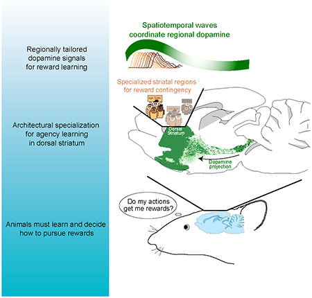
Significant evidence supports the view that dopamine shapes learning by encoding reward prediction errors. However, it is unknown whether striatal targets receive tailored dopamine dynamics based on regional functional specialization. Here, we report wave-like spatiotemporal activity-patterns in dopamine axons and release across the dorsal striatum. These waves switch between activational motifs and organize dopamine transients into localized clusters within functionally related striatal subregions. Notably, wave trajectories were tailored to task demands, propagating from dorsomedial to dorsolateral striatum when rewards are contingent on animal behavior, and in the opponent direction when rewards are independent of behavioral responses. We propose a computational architecture in which striatal dopamine waves are sculpted by inference about agency, and provide a mechanism to direct credit assignment to specialized striatal subregions. Supporting model predictions, dorsomedial dopamine activity during reward-pursuit signaled the extent of instrumental control, and interacted with reward waves to predict future behavioral adjustments.
Graphical Abstract
ETOC:
Dopamine axon activity and release across the dorsal striatum in mice exhibits wave-like spatiotemporal patterns tailored to task demands and predict an animal’s behavioral adjustments.
Introduction
Dopamine (DA) supports reward learning and motivated behaviors, but precisely what information it encodes and how it arrives at postsynaptic targets remains unclear (Berke, 2018; Berridge, 2007; Collins and Frank, 2014; Schultz, 2016). According to the reward prediction error (RPE) hypothesis, transients in DA signaling reflect deviations from reward expectation which drive reinforcement learning (RL) (Montague et al., 1996; Schultz et al., 1997). This formulation generally treats DA as a “global” (spatiotemporally uniform) signal, a view based on two key findings. First, DA axon projections to the forebrain are extensively divergent (Matsuda et al., 2009; Prensa and Parent, 2001), providing an architecture for broadcast-like communication. Second, midbrain DA neuron spikes are highly synchronized (Hyland et al., 2002; Li et al., 2011), putatively implementing a code for RPEs (Eshel et al., 2016; Joshua et al., 2009; Kim et al., 2012; Mohebi et al., 2019). These observations form the basis for an influential view (Glimcher, 2011; Kim et al., 2020; Schultz, 1998) of what DA communicates and how it is delivered: scalar RPEs that are uniformly broadcast to all recipient subregions.
It remains debated, however, if DA signals convey such scalar, uniform decision variables. In the midbrain, DA neurons are reported to encode multiple behavioral- and stimulus-specific features (Engelhard et al., 2019; Sharpe et al., 2018), or distributions of reward outcomes in an RPE framework (Dabney et al., 2020). Moreover, the major subregions of the striatum receive vastly different patterns of DA following unpredicted reward delivery (Brown et al., 2011), during motivated pursuit (Hamid et al., 2016; Shnitko and Robinson, 2015) and to conditioned stimuli (Menegas et al., 2017). If regional heterogeneity is an adaptive feature of striatal DA dynamics, what are the organizational rules for large scale DA transmission, and how do they facilitate computational/circuit operations in the service of behavioral flexibility?
An important clue is the functional architecture of hierarchical corticostriatal loops (Graybiel, 2008; Haber, 2003), wherein multiple striatal “actors” (or subregions) gate the selection of cortical actions at various functional levels of abstraction (Balleine et al., 2015; Frank, 2011). A global DA RPE would equally reinforce all of these circuits, leading to inefficient learning when only a subset of them are responsible for rewards. Indeed, in theoretical models, robust learning in complex tasks requires RPEs that are preferentially directed to “credit” striatal actors/subregions in proportion to the extent of their participation in action selection (Frank and Badre, 2012; O’Reilly and Frank, 2006). While such regional, actor-specific striatal RPEs are reported in human fMRI studies (Badre and Frank, 2011; Gershman et al., 2009), we currently lack an empirical demonstration of whether DA signals are tailored to subregions according to their functional/computational specialty. Here, we used widefield imaging to assay DA dynamics over large territories of the dorsal striatum. We report spatiotemporally heterogeneous DA responses characterized by wave-like patterns that are regionally tailored to striatal targets as a function of task demands and predict animal’s behavioral adjustments.
Results
Related striatal subregions receive correlated DA input
We set out to study the large scale organization of DA responses across the dorsal striatum (DS). Standard methods for DA assay have restricted spatial scale (10s - 100s of micrometers); we overcame these limitations by injecting cre-dependent GCaMP6f into the midbrain of DAT-cre mice and captured DA dynamics through a ~7mm2 chronic imaging window over the DS (Figure 1A). This approach provided optical access to 60-80% of the dorsal surface of the mouse striatum, with a view of dorsomedial (DMS), dorsolateral (DLS) and partial access to the posterior-tail (TS) region of the striatum (Figure 1B). A separate group of mice received striatal injection of fluorescent DA sensor, dLight, followed by window surgery. We combined DA activity indicators with the expression of tdTomato to simultaneously capture inert red frames under dual-color, head-fixed preparations at multiple levels of resolution with one- or two-photon microscopy.
Figure 1: DA dynamics are similar in nearby DS territories.
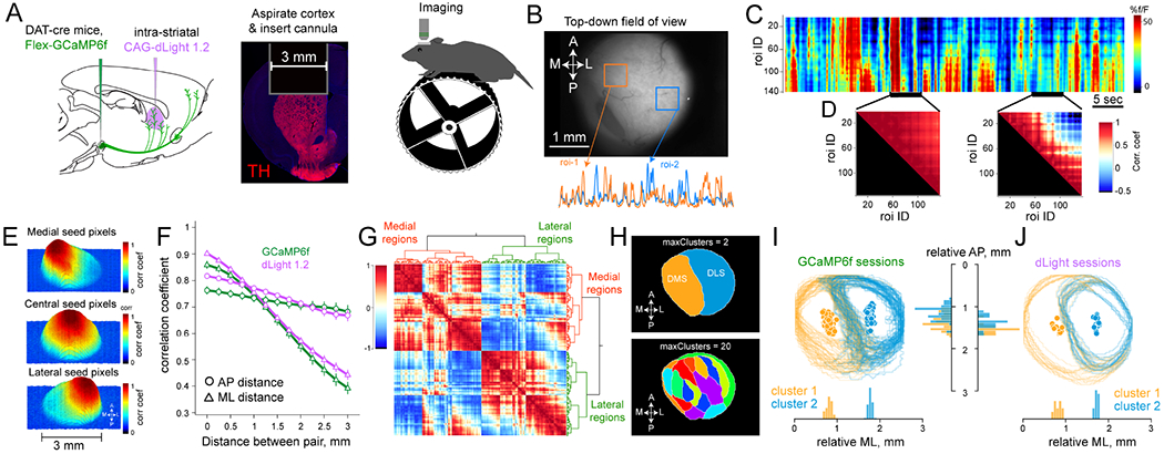
(A) Schematic of the methods to achieve DA imaging. Fluorophores are first virally transfected (left) and a 3mm diameter cannula (middle) was implanted after cortical resection for optical access to DS in head-fixed mice (right).
(B) Top-down field-of-view, and example GCAMP6f fluorescence from two DS regions.
(C) Heatmap of DA responses from multiple ROIs, sorted so that medial regions are at top, and lateral regions are at the bottom.
(D) Example correlation matrices of all ROIs during 5sec epochs highlighted in (C) demonstrating the evolution of regional correlation patterns.
(E) Correlation map of pairwise comparisons for GCaMP6f responses in one session. The top panel shows strength of coupling between medial pixels with all other areas. Middle and bottom plots show the same for central and lateral seed regions.
(F) Quantification of mean pairwise correlations as a function of distance, separated by mediolateral and anterior-posterior distances in the dLight and GCaMP6f signals. n=8 GCaMP6f mice, n=6 dLight mice. Error bars are mean ± SEM.
(G) Correlation matrix of one session sorted using hierarchical clustering to assess the regional similarity of DA input.
(H) Top, anatomical projection of regions that belong in the same cluster at highest dendrogram threshold, outlining medial and lateral subregions of the DS. Increasing the cluster threshold to 20 (bottom) revealed smaller, but anatomically contiguous regions of the striatum.
(I) Boundaries of the first two clusters identified in GCaMP6f sessions (n=58 sessions, 8 mice). Orange and blue circles indicate the centroid of identified clusters.
(J) same as (I) for dLight imaging (n=18 sessions, 6 mice).
We first focused on spontaneous DA signals in a dark chamber without external stimuli. To test whether DA responses are globally synchronized, we compared fluorescence signals in DS regions-of-interest (ROIs) (Figure 1B). While ROIs were sometimes globally synchronized, we observed evidence of decorrelated activity across striatal subregions that temporally evolved (Figures 1C–D). This regional variability was observed both in DA concentration and axonal calcium signals (dLight and GCaMP6f fluorescence), and also apparent on the micron scale of DA terminals (Figure S1A). Moreover, DA activity showed strong local correlations that gradually decreased with anatomical distance (Figures 1E and S1B), comparable to the organization of striatal spiny-neuron activity (Klaus et al., 2017; Parker et al., 2018; Shin et al., 2020). Strikingly, this distance-dependent falloff had a strong bias towards the medio-lateral axis (Figure 1F; two-way ANOVA with significant main effect of direction, F(1,7) = 82.3, P = 4.0×10⁻⁵ for 8 GCaMP6f mice and F(1,5) = 71.7, P = 3.7×10⁻⁴ for 6 dLight mice) that was not observed in simultaneously captured tdTomato frames (P > 0.4). Together, these results demonstrate that DA inputs can become recruited asynchronously (Howe and Dombeck, 2016), hinting that the global DA hypothesis may need to be refined.
To further examine the topographical organization of DS DA, we used standard clustering analyses (Figure 1G). In every dataset (n = 76 sessions from 8 GCaMP6f mice and 6 dLight mice), the highest cluster threshold identified two contiguous territories in the field-of-view (Figures 1H–J), outlining well-established DS subregions; medial (DMS) and lateral (DLS) striatum (Balleine et al., 2007; Graybiel, 2008; Yin and Knowlton, 2006). Increasing cluster limits progressively revealed smaller areas of DS (Figures 1H and S1F–G), resembling striatal subdomains previously identified based on glutamatergic input patterns and behavioral specialty (Hintiryan et al., 2016; Hooks et al., 2018; Hunnicutt et al., 2016; Matamales et al., 2020). We did not observe these territories when clustering control tdTomato frames, and shuffling the pixel-wise spatial (or temporal) order of GCaMP6f and dLight signals produced random clusters. Together, these results provide evidence for regional coordination of DA transmission and served as an initial basis for evaluating whether DA inputs are modulated by the underlying subregion’s computational specialty.
Wave-like patterns coordinate DA activity across the dorsal striatum
We next noted that the distance-dependence of correlated DA activity patterns reflected an underlying organization of spatiotemporally continuous trajectories. In particular, both GCaMP6f and dLight fluorescence initiated in localized striatal zones and migrated across DS as DA axons become sequentially recruited to affect DA release in spatially contiguous regions (Figures 2A and S2, Video S1). These trajectories, which we quantify below, resembled those described as traveling waves in cortical and subcortical brain regions (Grinvald et al., 1994; Lubenov and Siapas, 2009; Mohajerani et al., 2013; Muller et al., 2014, 2018). From here on, we use the ‘DA wave’ terminology as a shorthand to describe the spatiotemporally continuous, flow-like patterns of dopaminergic activity across DS.
Figure 2: Wave-like sequences of DA responses switch between motifs.
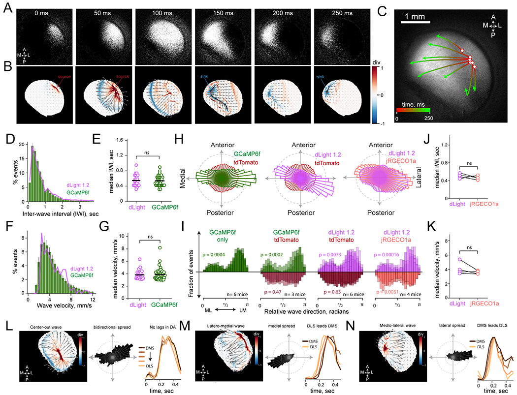
(A) Spatiotemporal activation of DA axons in an example GCaMP6f session (see Video S1). Frames acquired 50ms apart show activity initiated in lateral DS that progressively invades most of the FOV, before terminating in medial regions.
(B) Vector field (gray arrows) from optic-flow analysis of frames in (A). The color map depicts normalized divergence of the vector field at each pixel, visualizing source regions (red), and sink regions (blue).
(C) Streamlines of the detected DA flow across DS in (A) and (B) drawn from seed pixels indicated by white circles.
(D) Distribution of wave frequency in GCaMP6f sessions (green) and dLight sessions (purple).
(E) Median inter-wave-interval of each session for dLight, n=24 sessions, 6 mice, and GCaMP6f sessions, n=40 sessions, 8 mice. (P = 0.23; one-way ANOVA).
(F) Distribution of DA wave propagation velocities, data same as (D) and (E).
(G) Median wave velocity for dLight and GCaMP6f sessions, same data as (E). (P = 0.19; one-way ANOVA).
(H) Wave direction distributions in representative sessions under multi-color imaging conditions. The panels summarize DA trajectories in mice expressing GCaMP6f/tdTomato (left), and dLight/tdTomato (middle) and dLight/jRGECO1a (right).
(I) Overlayed, linearized distributions of wave directions from each mouse. P-values are for the Omnibus test for whether angles are uniformly distributed.
(J) Comparison of dLight and jRGECO1a median inter-wave-interval, n=4 mice (P = 0.4; one-way rmANOVA).
(K) Comparison of dLight and jRGECO1a wave velocity, n=4 mice (P = 0.25; one-way rmANOVA).
(L) Center-Out waves are centrally sourced (left panel), have bidirectional propagation directionality (middle panel), and produce a synchronized increase in DA across the ML axis of DS (right panel).
(M) Latero-medial waves, same format as (L).
(N) Mediolateral waves, same format as (M). Error bars and shading in (D) and (F) indicate SEM.
To quantitatively characterize these DA trajectories, we leveraged optic flow algorithms that extract frame-by-frame flow fields (Afrashteh et al., 2017; Townsend and Gong, 2018) (see Methods for details). The transient activation in DA axons (and release) originated from spatially clustered ‘source’ regions defined by divergent vectors that signify outward flow (Figures 2B and S2A). Once initiated, fluorescence migrated to neighboring striatal regions before terminating as a result of flow toward ‘sink’ locations (Figure 2B). DA waves entered the dorsal striatum with exponentially decaying inter-wave-intervals (Figures 2D–E) and propagated with a range of velocities (Figures 2F–G). Moreover, the overall direction of flow was bimodally distributed (Figures 2H–I; Omnibus test for angular uniformity; GCaMP6f sessions P < 10−4, dLight sessions P < 10−3), significantly biased to a medial-lateral propagation axis, that was not present in simultaneously acquired tdTomato frames (Figure 2I; P > 0.4).
The flow-like property exhibited similar statistics for DA axon activation and release (Figures 2E–G), indicating that axonal excitation and release may be coupled. To concretely test this possibility, we made dual-color widefield recordings in 4 DAT-cre mice with cre-dependent jRGECO1a injected into the midbrain and dLight broadly expressed in the DS (Figure S3A). Indeed, we found strong coupling between the simultaneously acquired dLight and jRGECO1a spatiotemporal flow patterns (Figures 2J–K, S3B–D), with highly correlated temporal dynamics in the major striatal subdivisions, that was not affected by the locomotor state of the mice (Figure S3E–F).
We also examined if the complex DA trajectories resulted from various imaging artifacts and/or damage to cortex and glutamatergic afferents during surgery for cannula implantation. We first ruled out the contribution of imaging artifacts related to locomotion and blood flow by imaging multiple DA activity sensors with spectrally separated inert fluorophores that did not display fast, spatially heterogeneous fluctuations (Figures 2I and S3G–J). Second, we confirmed similar flow-like, sequential DA signals in absence of cortical resection in a separate group of animals that received small-diameter optic fibers arranged into a grid (Figures S3K–S) to minimize cortical damage. These findings lead us to conclude that wave-like activation patterns reflect a striatal DA circuit-specialization for spatiotemporally coordinated dynamics.
Motif waves implement systematic DA phase-shifts across dorsal striatum
The propagation of wave-like dynamics could produce temporal delays in the arrival of DA transients across the striatum that in turn, may regulate regional DA-dependent plasticity mechanisms (Iino et al., 2020; Shindou et al., 2019; Yagishita et al., 2014). We asked whether elementary propagation trajectories could realize assorted temporal lead/lags in DA activation across DS. Using multiple convergent methods for the analysis of spatiotemporal sequences (Mackevicius et al., 2019; Townsend and Gong, 2018), we identified rudimentary motif patterns that affect DA dynamics across the DS (Figures S2F–H, Video S3). We focused our analyses on three motif waves that produced 93 ± 3% of the DA transients (Figure S2H). First, Center-Out (CO) waves initiate at the juncture of DMS and DLS and rapidly spread bilaterally outward to produce DA signals that arrive at different striatal regions with little delay (Figure 2L). Second, Latero-Medial (LM) waves start from the lateral striatum and predominantly propagate medially to deliver delayed DA transients to the DMS relative to DLS (Figure 2M). Third, Medio-Lateral (ML) waves are sourced in the DMS and propagate laterally, activating DA axons in the medial striatum first and progressively recruited DA in lateral regions (Figure 2N). These findings demonstrate that motif waves specify how DA responses initiate and propagate across DS, codifying the relative timing of regional DA that may shape striatal plasticity.
Rewards evoke directional DA waves
What is the functional role of DA waves in adaptive behavior? We set out to determine the computational significance of DA trajectories in the context of the well-studied role of DS in instrumental behavior. The DS exhibits graded behavioral specialty, with the DMS implicated in agentic, goal-directed behaviors involving action-outcome learning, and DLS in stimulus-response behaviors (Yin and Knowlton 2006; Balleine et al. 2007; Corbit and Janak 2010; Thorn et al. 2010). Inactivation or manipulation of DA in DMS degrades goal-directed planning and action due to an inability to learn whether rewards are under instrumental control (Balleine and O’Doherty, 2010; Wunderlich et al., 2012).
To study whether DS DA is tailored to the target region’s computational specialty, we designed two operant tasks that manipulated action-outcome contingency and asked whether DA dynamics carry information about instrumental controllability (i.e., agency). Auditory tones that escalated in frequency indicated progress to rewards in both tasks (Figures 3A–D). In the “Instrumental” task, this reward progress was contingent on, and tied to, the mouse running on a wheel to traverse a linearized distance. The distance to reward was randomly selected from a uniform distribution on each trial (50-150 cm, Figure 3C). Thus, while the mouse was in control of tone transitions, the specific contingencies varied across trials. In a second ‘Pavlovian’ task, mice were free to run, but the tone transitions occurred independent of running, and the time to reward was drawn from a uniform distribution (4-8 sec, Figure 3C). Thus, the two tasks differed in instrumental controllability but were structurally identical: Tones provided information about progress to reward, which could not be inferred from elapsed time alone. Trained mice exhibited anticipatory lick trajectories that increased with ascending tone frequency in both tasks (Figures 3E–F), indicating that mice used escalating tones to update their online judgment of progress to reward. Moreover, analysis of run bouts across the two tasks revealed that mice invested goal-directed effort to receive rewards selectively in the instrumental task (Figure S4).
Figure 3: Reward promotes directional waves depending on instrumental requirement.
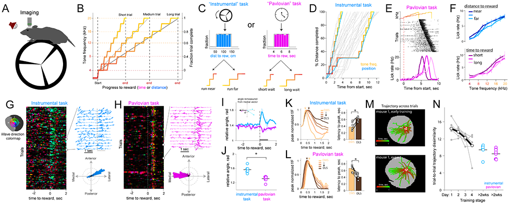
(A) Schematic of the test chamber.
(B) Escalating tone frequencies indicate progress to rewards delivered at end.
(C) Schematic of the two task variants. Wheel running advances tones instrumental task and the specific distance is randomly drawn from a distribution (left panels), whereas mere passage of time advanced tones in the Pavlovian condition (right panels).
(D) Example trials in the instrumental task showing that faster wheel running advanced tones rapidly, whereas a transient pause in running halts tone frequency change.
(E) Example licking behavior in one Pavlovian session sorted by delay to reward. Mice increase anticipatory licking as they get closer to reward, in short, medium, and long trials (shades of color).
(F) Mean anticipatory licking during trial progress in instrumental (top) and Pavlovian sessions (bottom), broken down by trial length. (P < 0.001 for effect of tone, P = 0.9 for effect of distance in instrumental sessions; P = 0.001 effect of tone, P = 0.4 effect of tone in Pavlovian; two-way ANOVA).
(G) Reward-aligned DA wave trajectories in an example GCaMP6f instrumental session (n=92 trials). Color hue indicates wave direction (top left inset) and saturation indicates flow magnitude. Top right panel shows quiver plots of a subset of trials, and the bottom angular plot shows the session’s wave direction distribution quantified in a 1sec window after reward.
(H) Reward wave for a Pavlovian session (n=77 trials), same format as (G).
(I) Linearized wave angle at reward in instrumental (n=6 mice, 139±18 trials per mouse), and Pavlovian sessions (n=8 mice, 108±12 trials SEM per mouse).
(J) Quantification of relative wave directions in the two tasks, n=6 instrumental and 8 Pavlovian. (P = 1.1 × 10⁻⁴; One-way ANOVA).
(K) Peak normalized reward fluorescence across DS in instrumental condition. Right panel shows mean latency-to-peak DA at reward in DMS and DLS (P = 0.031; Wilcoxen test).
(L) Same as (K) for Pavlovian task (P = 0.007; Wilcoxen test).
(M) DA flow trajectories at unpredicted reward early (top) and late (bottom) in training. Each line represents flow trajectory in a trial from a seed location (white circles, n=70 trials).
(N) Variability of trial-by-trial DA trajectories declines across 4 days of reward exposure (P = 0.018, effect of day; One-way rmANOVA, n=6 mice). Error bars in (F) and (I) represent SEM.
As in the spontaneous conditions reported above, DA waves were ubiquitous during task performance and were especially prevalent at reward. Notably, reward delivery immediately resynchronized DA responses into propagating waves that had opponent directions depending on task conditions. Specifically, rewards after an instrumental trial triggered medially sourced, laterally propagating (medio-lateral, ML) waves (Figures 3G–J, Video S4), whereas rewards in the Pavlovian task promoted laterally initiated, medially propagating (latero-medial, LM) waves (Figures 3H–J, Video S4). These divergent responses in the two task conditions affected the temporal order of DA recruitment on the mediolateral axis: DMS achieved peak reward-induced DA significantly sooner than lateral regions in the instrumental condition (Figure 3K; P = 0.031, Wilcoxon Signed-Rank test; n = 6 mice), whereas, DMS had delayed DA peaks in the Pavlovian task (Figure 3L; P = 0.0078, Wilcoxon Signed-Rank test; n = 8 mice). Moreover, these wave trajectories evolved with task experience, with reward-induced waves exhibiting irregular trajectories in naive animals but becoming more consistent and directional across several training days (Figures 3M–N, Video S5).
Wave-like dynamics support graded credit assignment in RL simulations
The dynamic sculpting of these trajectories by training and task demands suggested that DA waves may be important for behavioral flexibility. In particular, the continuous propagation of DA across the striatum in space and time motivated a revision of standard “temporal-difference (TD)” RL models wherein a single reward-value influences learning about reward-predictive events. We reasoned that these views could be expanded to include “spatiotemporal differences” in which waves carry additional, graded information about structural sub-circuits that are most likely to be responsible for rewards. To formally explore this account, we simulated the consequence of spatially delayed rewards in the tone tasks within a TD framework. The simulation contained a bank of parallel agents representing striatal subregions (Frank and Badre, 2012) (Figure S5), and tone/state transitions formulated as sequential semi-Markov states (Daw et al., 2006). To explore the consequence of mediolaterally propagating waves, the reward response for the most ‘medial’ agent was delivered immediately at the end of the trial, and progressively delayed for more ‘lateral’ agents. The model also included eligibility traces (Singh and Sutton, 1996; Sutton and Barto, 2018) so that any delays in rewards could still be attributed to earlier states that were no longer active, in proportion to their decaying eligibility. This choice was motivated by both computational principles and the documented impact of such delays in DA signaling on synaptic plasticity in mouse striatum (Shindou et al., 2019; Yagishita et al., 2014).
As learning progressed across trials, the RPE response in the most medial agent back-propagated to the earliest predictor of reward (Montague et al., 1996)(Figure S5, Video S7). However, in more lateral agents, delays in reward response led to progressively reduced credit assignment to the earlier states. Indeed, these effects translated to produce steeper Value functions in the most medial agents as the agent progressed to reward, and lateral agents shallower ramps (Figure S5). Given that the Value function reflects the reward value of the agent’s predictions, which can be used to guide action selection, these simulations provide an initial algorithmic demonstration that reward-induced waves can give rise to asymmetric structural credit assignment. Moreover, as rewards produced opponent DA wave dynamics across the two tasks, this mechanism would preferentially reinforce the medial DS agents for instrumental tasks. We next test this prediction in mouse behavior before examining how instrumental controllability may be computed in these tasks to affect wave dynamics.
DA waves track changing task contingencies and predict behavioral adaptation
For our behavioral tasks, we posited that opponent DA waves would facilitate reward-credit dissemination to specialized striatal regions depending on the animal’s instrumental agency in advancing progress to reward. This hypothesis is inspired by expert-like organization of DS anatomy (Aoki et al., 2019; Hintiryan et al., 2016; Hunnicutt et al., 2016; Matamales et al., 2020), activity (Barbera et al., 2016; Kasanetz et al., 2008; Klaus et al., 2017; Parker et al., 2018; Piray et al., 2017; Shin et al., 2020), and graded specialization for action-outcome learning on the mediolateral axis (Balleine and O’Doherty, 2010; Graybiel, 2008; Kim and Hikosaka, 2015; Parent and Hazrati, 1995; Thorn et al., 2010; Yin and Knowlton, 2006). Testing this possibility required task-conditions wherein agency is dynamically manipulated in the same session. We thus trained a separate cohort of mice in a serial reversal task with changing reward contingencies across ‘instrumental’ and ‘Pavlovian’ blocks lasting 25-35 trials each (Figure 4A). Mice experienced multiple unsignalled reversals in the same session, requiring continuous learning about agency. We predicted that reward-epoch DA trajectories should: i) reverse directions after block transitions; and ii) predict the animal’s future behavioral adjustments, with ML waves signaling agency and increase future running.
Figure 4: Within-session reversal of task contingency shifts DA wave directions dynamically.

(A) Schematic of the test chamber.
(B) Velocity changes as mice transitioned instrumental to Pavlovian blocks (black) or vice-versa (gray).
(C) Quantification of mean velocity in the two blocks (P = 1.9×10⁻⁵, effect of trial-type; one-way rmANOVA, n=15 sessions from 6 dLight and 4 GCaMP6f mice).
(D) Reward aligned DA trajectories (same format as in 3G) across block transitions in a dLight session (n=122 trials). Right panel shows quiver plot flow vectors of a subset of trials at block change.
(E) Linearized, trial wave angles in 1sec window after reward. Same data as (D).
(F) Summary of linearized wave direction in Pavlovian trials (n=58 trials) and instrumental trials (n=64 trials).
(G) Same data as (F), showing the angular distribution of wave angles.
(H) Wave direction reversals across block transitions in 5-trial bins. Data combined across GCaMP6f and dLight sessions. Same format as (B), n=15 sessions from 6 dLight and 4 GCaMP6f mice.
(I) Quantification of wave mean reward wave directions for GCaMP6f, dLight, and tdTomato (respectively, P = 0.002, P = 0.016, P = 0.4 for effect of trial-type; one-way rmANOVA).
(J) Reward wave directions separated by run velocity in instrumental and Pavlovian blocks (P = 0.001 effect of velocity bin, P=0.004 trial-type X velocity interaction; two-way rmANOVA). Data same as (H).
(K) Breakdown of wave direction by congruence between running and trial progress combined across GCaMP6f and dLight sessions. (main effect of Velocity F(5,70) = 4.5, P = 0.001 with significant Trial-type x Velocity interaction F(5,70) = 3.81, P = 0.004; Two-way rmANOVA)
(L) Data from an example reversal session showing effect of past reward wave direction on run speed. Trials were separated by 3 wave direction bins, same data as (E).
(M) Correlation between last-trial reward wave angle and velocity for 15 sessions (r = 0.2, P = 0.002 in instrumental trials and r = 0.43, P < 10−5 in Pavlovian trials).
(N) History-dependent regression of wave angle on future-trial velocity ( r = 0.34, P = 0.007 Spearman’s rank correlation of coefficients, model R2 = 0.44, n=15 dLight and GCaMP6f sessions; betas not significant and model R2 = 0.48 for tdTomato frames).
Trained mice completed an average of 6.4±0.3 reversals across 210±10 trials per session and dynamically adjusted their performance according to task contingencies. Specifically, mice completed instrumental blocks with a significantly higher run velocity and ramped down their velocity after they entered Pavlovian blocks (Figures 4B–C). Replicating our previous findings in a different cohort of mice, we observed robust DA waves following instrumental and Pavlovian trials at reward delivery (Figures 4D), with ML waves in instrumental trials and LM waves following Pavlovian trials (Figures 4E–G). The wave reversals persisted across multiple block transitions (Figure 4H) for both axonal activation and DA release, but were not observed in tdTomato frames (Figure 4I). The wave dynamics were not simply related to differences in motoric output or velocity: opponent wave directions were observed even when velocities were matched across tasks (Figure 4J). Moreover, in Pavlovian trials with elevated running velocity, wave directions were influenced by the locomotion-sensory congruence, defined as the correlation of wheel displacement and distance to reward in 250ms bins. In particular, we found that spurious correlations between sensory evidence and (non-contingent) advance to reward in high-velocity Pavlovian trials promoted ML waves (Figure 4K), indicating that wave directions are shaped by spurious evidence for instrumental control. These results support our prediction that DS wave trajectories are sensitive to task demands across the two conditions.
While these results confirm that wave trajectories dynamically shift across task contingencies, they do not establish whether they are involved in future behavioral adjustments. We thus tested whether DA wave directions at reward predict future-trial running in a history-dependent manner. We found that past wave angles were related to next-trial running speed (Figure 4L), and significantly correlated with run velocity in successive trials (Figure 4M). Moreover, the effect of past wave directions on next-trial velocity had a history dependence, with more recent-trial DA wave directions demonstrating the largest velocity regression coefficients (Figure 4N), a pattern not observed in tdTomato frames. These results are reminiscent of the impact of reward history in canonical RL models and data (Bayer and Glimcher, 2005; Lau and Glimcher, 2005; Sutton and Barto, 2018) and support our second prediction. Together, our observations support the conclusion that DA wave trajectories are sensitive to evidence for agency, and deliver opponent DA responses that predict the animal’s behavioral adjustments according to task demands, manifested as adaptive running speed.
A Mixture of Experts RL model for inferring agency and guiding DA waves
The above data support general predictions about the role of opponent DA trajectories in instrumental learning by directing reward credit to (and away from) DMS regions specialized for agency. However, these findings do not reveal how the mouse and the DA system infer controllability. In our tasks, the animal must make the critical inference of whether it controls reward-predictive tone transitions and which specific contingency (i.e., distance to run to advance tones) applies in the current trial. Thus, for mice to learn about agency and dynamically adjust their behaviors, the trial-by-trial evidence for instrumental control should determine whether reward-evoked DA will strengthen action-outcome learning (i.e., favor the DMS). In other words, online evidence for agency prescribes wave direction, that in turn promotes (or suppresses) instrumental performance in subsequent trials. To formalize this notion, we constructed a hierarchical multi-agent mixture of experts (MoE) model, building on earlier models of corticostriatal interactions in learning and action (Doya et al., 2002; Frank and Badre, 2012) (Figures 5A and S6). We first summarize the model’s components (see Methods for details) before outlining and testing precise predictions related to DA dynamics and behavior.
Figure 5: A mixture-of-experts RL model.
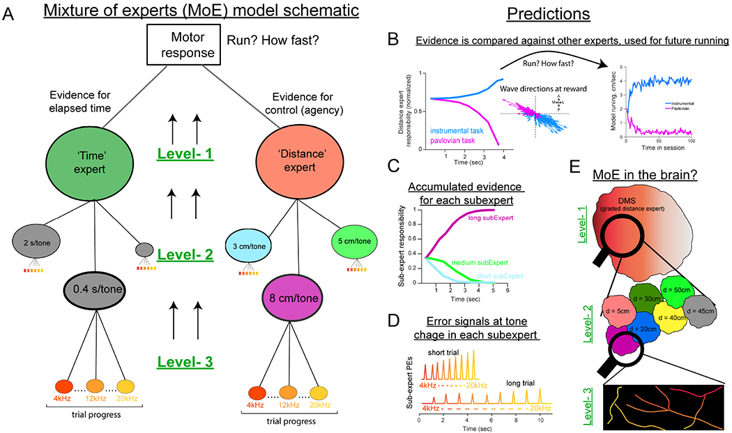
(A) Schematic of MoE model. The agent decides to run based on evidence from ‘Distance’ or ‘Time’ experts (level-1) that rely on subordinate ‘sub-experts’ that specialize in specific contingencies (level-2). Each sub-expert experiences a trial as a series of tone/state transitions (level-3).
(B) Model predictions at level-1; experts accumulate evidence across the two tasks. Accumulation of responsibility in the ‘distance’ expert is used to adjust model velocities and also direct waves at reward.
(C) Level-2; each sub-expert will accumulate evidence according to their specialty.
(D) Level-3; sensory observations (tone/state changes) induce errors if not aligned with “sub-expert” prediction.
(E) Proposed reflection of MoE signals in striatal DA activity with DMS representing evidence for control (level-1), is enriched with subregions tuned to specific contingencies (level-2), and sPEs are signaled by DA axon segments (level-3).
At the highest layer (level 1) is an ‘expert’, putatively corresponding to DMS, that computes evidence that the agent is in control of outcomes (i.e., that its actions cause tone transitions and rewards). To do so, this expert must consider multiple potential action-outcome relationships, given the distribution of time/distance contingencies experienced in the task (Figure 5A). As such, the expert has access to multiple sub-experts within its domain (level 2), each specialized to represent different contingencies (e.g., the distance needed to run is short, medium, or long trials). The expert can recruit the sub-expert that best predicts the state transitions in the current trial (i.e., the one with the smallest reward prediction errors, minimizing the Bellman error). Moreover, auditory tone transitions that occur earlier or later than predicted give rise to sub-expert reward prediction errors (sRPEs; level 3). For example, during a short distance trial, the ‘short-distance’ sub-expert experiences reduced sRPEs, whereas a ‘long-distance’ sub-expert experiences large sRPEs at tone transitions that occur earlier than expected. At the end of a trial, reward credit is delivered to experts that are most predictive of state transitions, which will guide future model “running”. Finally, the agent will increase its speed only when the accumulated evidence is larger for agentic “Distance” experts than non-agentic “Time” experts.
This formulation allows an agent to learn and flexibly adapt behavior based on task contingencies (Figure S6) (Doya et al., 2002; Frank and Badre, 2012) and expands the RL account of striatal DA such that it is informed by the inferred causal contributions of recipient subregions (Chang et al., 2004; Gershman et al., 2015; O’Reilly and Frank, 2006; Russell and Zimdars, 2003). Thus, in contrast to previous global scalar DA accounts, our model provides a formal framework for adaptive DA signals that are spatiotemporally tailored to striatal subregions. Moreover, this architecture makes multi-level predictions about DA dynamics during the reward pursuit and outcome epochs (Figures 5B–D and S6), potentially tying together the role of DA in performance and learning. We systematically test three key predictions from the model below.
DA ramps in DMS signal evidence for agency and predict subsequent reward dynamics
If DA waves at reward guide spatiotemporal credit assignment, what determines which subregion should receive the credit? As noted above, the model contains a DMS-like “distance expert” that accumulates online evidence for agency in the form of ramping signals that are proportional to the accuracy of underlying subregions’ predictions (Figure 5B). Ramping DA signals during reward pursuit in the midbrain and ventral striatum have been described as scalar decision variables corresponding to RPEs (Gershman, 2014; Lloyd and Dayan, 2015; Morita and Kato, 2014), Value functions (Hamid et al., 2016), or progress within a cognitive map (Guru et al., 2020). Instead, we posit here that anticipatory DA ramps in a given DS subregion reflect the accuracy or usefulness of the underlying regions’ predictions about task contingency, thus providing a tag for how much reward-credit it should receive at outcome. Thus, our model predicts that anticipatory epoch DA dynamics also diverge across striatal subregions and task demands.
We tested this prediction by examining DA activity during anticipation as mice drew closer to reward. In the instrumental task, we observed a buildup of activity in the DMS (Figure 6A–D), ramping in proportion to the progress to reward (Hamid et al., 2016; Howe et al., 2013). Strikingly, the opposite profile was observed in the Pavlovian condition with negative ramps even as mice drew closer to rewards (Figures 6B–D). The opponent DMS ramp slopes were also observed in blockwise reversal sessions, with dLight and GCaMP6f ramps dynamically reversing after block change (Figures 6E–G), but not in tdTomato frames (Figure 6G).
Figure 6: Anticipatory epoch DA reflects inferred controllability and predicts DA delays at reward.
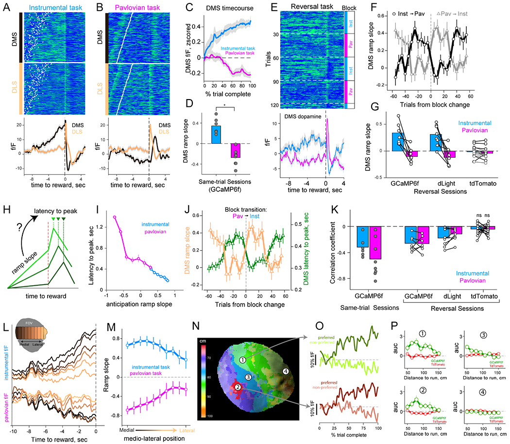
(A) Anticipation- and reward-epoch DA fluorescence separately for DMS and DLS in an instrumental session. Data sorted by distance to run, white dots indicate trial-start.
(B) Same format as (A) for a Pavlovian session, sorted by time to reward.
(C) Z-scored ramp profile as a fraction of trial complete in DMS from two tasks (n=6 instrumental sessions and n=8 for Pavlovian).
(D) Quantification of ramp slopes in GCaMP6f expressing mice (effect of task-type P = 10−6, one-way ANOVA).
(E) DA dynamics in the DMS of GCaMP6f signals in one reversal session. Block-type is indicated at right, bottom panel shows mean fluorescence across the trial types.
(F) DMS ramp slopes across block transitions. Same data and format as Figure 4H.
(G) Quantification of mean ramp slope in reversal sessions (effect of trial-type P=0.004 for GCaMP6f, P=0.04 for dLight, P=0.67 for tdTomato;One-way rmANOVA).
(H) Proposed relationship between ramps and reward peak.
(I) Relationship of ramp-slope and peak-latency in DMS in one representative instrumental and Pavlovian session each. Note inverse relationships across both.
(J) Trial-by-trial relationship between ramp-slope and peak-latency in DMS of mice exposed to reversal session. Same data and format as (F).
(K) Quantification of session correlation between ramp-slope and peak-latency (P=0.03 for instrumental-only and P=0.007 Pavlovian-only sessions; Wilcoxen test).
(L) Anticipatory ramps in example instrumental (top) and Pavlovian (bottom) sessions broken down by ROIs along the mediolateral axis (inset).
(M) Quantification of mediolateral expression of ramp slopes (effect of ML position P=2.1×10⁻⁴ instrumental only sessions, P = 1.9x10⁻⁵ for Pavlovian only session; One-way rmANOVA. For reversal sessions, P = 5.4×10⁻⁴; two-way rmANOVA).
(N) Map of distance contingency specialization in DS subregions in one instrumental GCaMP6f session. Color indicates distance requirement associated with the steepest ramp of each pixel.
(O) Example timecourses of preferred and non-preferred trial ramps in example subregions.
(P) Quantification of the area-under-curve of anticipatory dynamics across distance contingencies for simultaneously acquired GCaMP6f signals (green) and tdTomato (red) in four example striatal regions (highlighted in (N).
Shading and error bars represent SEM
The opposite profile of anticipatory DA signals across the two task conditions is not explained by extant models of midbrain or accumbens DA ramps. Instead, we interpret DS DA ramp dynamics as reflecting the value of the underlying subregion’s agentic predictions, providing a marker for this region’s reward responsibility. In addition, because reward credit should be proportional to the accuracy of these agentic predictions, our interpretation ties together opponent anticipatory-dynamics with the opponent reward-waves. We specifically posited that if DA ramps relay the subregion’s reward-predictive accuracy, they would impact the subsequent timing of DA increases at reward, with regions assigned the most credit receiving the earliest DA bursts at reward. As such, trials with steepest ramp slopes (highest responsibility) should receive reward responses soonest (largest credit, Figure 6H). Consistent with this interpretation, we observed that DMS ramp slopes were inversely correlated with the latency-to-peak fluorescence following reward for both task conditions (Figures 6I–K). The negative relationship between DMS ramp slope and latency to reward-peak was also observed in DA dynamics of contingency-reversal sessions (Figures 6J–K; P < 10−4 for both GCaMP6f and dLight sessions), but not in simultaneously captured tdTomato frames (Figure 6K). These findings indicate that anticipatory DA dynamics in DMS are modulated by instrumental contingency and predict regional reward responses, demonstrating a relationship between eligibility and reward credit.
Regional DA ramps tailored to instrumental contingencies
Thus far, we have focused on the coarsest division of labor related to the highest level in our model (controllability, level-1), but the agent’s ability to infer control depends on underlying sub-experts that learn distinct action-outcome contingencies (level-2). Such a hierarchical scheme implies that within the DMS, smaller subregions should differentially express DA ramps for different distance contingencies. Indeed, we observed that DA ramp slopes were expressed across the mediolateral axis of the striatum to different extents (Figures 6L–M). We next tested whether territories of the DS exhibit specialized ramp profiles for different distance conditions, and found that contiguous striatal regions expressed steepest DA ramps for a preferred set of trials with related distance requirements (Figures 6N–P and S7A). We did not observe this regional contingency preference in simultaneously acquired tdTomato frames (Figure 6P). These results are consistent with previous studies on progressive instrumental specialization of DS on the mediolateral axis (Matamales et al., 2020; Thorn et al., 2010), and support our MoE interpretations that DMS consists of smaller subregions that learn, and express predictions for a variety of potential instrumental contingencies.
Reward-predictive sensory events evoke DA transients reminiscent of sub-expert RPEs
At the smallest scale (level-3), the ‘evidence’ for each sub-expert is accrued based on the degree to which they experience reward prediction errors (sRPEs) at state transitions (Figure 5D). In the model, each auditory tone is represented as a unique state within a sub-expert’s semi-Markov process, and sRPEs arise at tone transitions that occur earlier (or later) than expected. Thus, evidence for a given sub-expert is signaled by the relative lack of sRPEs compared to other sub-experts. This account predicts that tone transitions would give rise to rapid DA deflections reflecting sRPEs, and that these signals would be modulated by trial-length and position of tone within a trial. Specifically, the model predicts that: i) sRPEs would be larger in shorter trials (because tone transitions are indicative of future reward arriving earlier than expected), and ii) within a given task contingency, tones arriving later in the trial would drive larger deflections than early-trial tones due to temporal discounting (Figures 7A and S7).
Figure 7: Tone transition DA responses both in the widefield and 2-photon preparations.
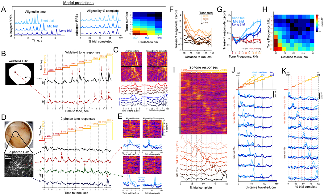
(A) Model predicted dynamics of sRPEs in different trial lengths and tone indexes.
(B) Average DA responses in two pixels from widefield imaging, aligned to each tone-change. Arrows indicate DA recruitment by tone change.
(C) Realignment of data in (B) as duration-sorted trials in a reversal session. Top set of trials in heat plots are Pavlovian trials and lower trials are Instrumental trials.
(D) Schematic and responses from 2-photon DA axon segments in an instrumental session (same format as (B).
(E) Alignment of 2p responses in time or fraction of trial completed. Average traces are broken down by trial distance.
(F) Quantification of widefield response magnitude for various trial contingencies and tone change (n = 2 mice).
(G) Same data as (F) visualized for three distance bins in GCaMP6f (blue lines) and tdTomato frames (red lines).
(H) Combined quantification for distance contingency and tone frequency.
(I) Activity of GCAMP6f in DA axon segments that respond to tone transitions during anticipation. Data (n= 106 trials) from multiple regions are realigned to fraction-trial-completed and concatenated. Bottom traces show the timecourse of each sPE group modulated by tones.
(J) Transient response-peaks in 2p data are not tuned to distance traveled. Note that the peak response appears at different x positions on the axis.
(K) Data in (J) realigned by tone position or fraction completed and broken down by distance contingency.
Supporting these predictions, we observed abrupt DA responses at tone changes in both widefield, one-photon (Figure 7B) and two-photon (Figure 7D) preparations. Specifically, individual pixels during widefield DA imaging responded to multiple tone changes, and consistently accompanied the sensory indicators of progress to reward (Figure 7C). In contrast to these multi-tone responses in individual pixels of the widefield data (Figure S7B–E), we noted that DA axon segments in the 2-photon condition reliably responded to single tone transitions (Figure 7E), and different portions of the imaged axon lattice tiled the full sequence of escalating tones (Figures 7I and S7F). Next, we assessed if these DA signals exhibited properties of sRPEs outlined above (i.e., trial length and position of tone in trial and not just sensory events or elapsed time; Figure 7A). Indeed, tone-responsive GCaMP6f and dLight pixels in the widefield were significantly modulated by trial length, with larger responses in short-distance conditions (Figures 7F–H). Moreover, these transients scale according to the position of the tone-transitions within a trial, a result not observed in the control frames (Figure 7H). The DA axon responses in the 2-photon condition were also modulated by trial distance contingency, and tone position in trial (Figures 7J–K). Together these observations indicate that sRPEs are represented in rapid DA responses at state transitions during anticipatory epoch, consistent with our model predictions.
Discussion
Our observations provide evidence for a spatiotemporal organizing principle of striatal DA signals and their behavioral relevance. Wave-like DA activation patterns were expressed as directional motifs that regulated the relative timing of regional DA changes and served to correlate DA in functionally related striatal territories. We reasoned that the computational significance of these waves in RL might be to assign spatiotemporal credit to striatal subregions differentially. Indeed, temporal delays on a similar timescale to those induced by DA waves are reported to constrain corticostriatal plasticity in vitro (Yagishita et al., 2014). Our TD simulations show that such temporal lags in reinforcement signals can drive spatially-asymmetric reward learning and credit assignment. Thus, as hierarchically recruited striatal subregions exhibit graded functional specialization (Hooks et al., 2018; Kasanetz et al., 2008; Klaus et al., 2017; Piray et al., 2017; Thorn et al., 2010), DA waves may serve to regulate plasticity in postsynaptic domains with diverse functional specialization.
We tested this hypothesis according to the documented specialty of DMS in action-outcome learning and goal-directed behaviors. Our tasks manipulated reward controllability, requiring mice to dynamically learn about agency. Consistent with our hypothesis that DMS DA dynamics would be tailored to task demands, we found that reward-delivery triggered DA waves in opponent directions based on task contingency. Mediolateral waves that produce rapid DMS DA peaks were enriched in instrumental trials, whereas lateromedial waves were prevalent following non-contingent Pavlovian trials. Notably, these wave directions reversed within a few trials after task reversal, and predicted future-trial behavioral adjustments with history-dependent effects in line with reinforcement learning. Together, our studies provide evidence for the role of spatiotemporal propagation of DA in agency learning by codifying the relative timing of a corticostriatal plasticity modulator.
Evidence for a computational model of regionally tailored DA signals
The mixture-of-experts (MoE) model served to formalize our empirical observations, building on hierarchical neural network models of corticostriatal interactions (Collins and Frank, 2013; Frank and Badre, 2012; O’Reilly and Frank, 2006). The model captures regional reward credit assignment in functionally specialized cortico-BG loops, inspired by previous anatomical and functional reports (Aoki et al., 2019; Barbera et al., 2016; Haber, 2003; Hintiryan et al., 2016; Hunnicutt et al., 2016; Klaus et al., 2017; Lee et al., 2020; Mandelbaum et al., 2019; Marquand et al., 2017; Märtin et al., 2019; Matamales et al., 2020; Parker et al., 2018; Shin et al., 2020; Stanley et al., 2020; Tanaka et al., 2004; Thorn et al., 2010). In the MoE, evidence for instrumental controllability was accrued in the form of ramps to the DMS expert. In particular, as a trial progressed, sub-experts experienced prediction errors (sRPEs) when sensory events did not align as expected based on their specialization. Conversely, congruence between actions and predicted outcomes for a given sub-expert led to progressive ramps signaling their prediction-accuracy and responsibility for impending rewards. In turn, these anticipatory ramps in the model will bias reward credit to ‘distance’ experts to increase the agent’s motoric output during the instrumental task but reduced running in the Pavlovian task.
Consistent with the MoE account, we reported anticipatory epoch DA ramping dynamics within large DMS regions that reversed directions between task conditions. Additional specialization was observed for distinct contingencies within smaller striatal subregions in the two tasks, consistent with sub-experts. We reasoned that these dynamics may serve a dual purpose. First, they could promote online behavioral-vigor flexibility according to the inferred task contingencies in the current trial. Second, these ramps could also signal which subregions were best predictive of reward outcomes, providing a tag for their responsibility (akin to an eligibility trace in RL (Singh and Sutton, 1996)). Such a tag would allow RPEs to preferentially credit the appropriate subregion and the eligible MSNs within it. While the two functions are not mutually exclusive, our data provide strong support for the second interpretation: On a trial-by-trial basis, the degree of ramping in a given subregion was predictive of the latency to reward peak elicited by the wave. Moreover, the ramp slope and wave direction were predictive of subsequent-trial behavioral adjustments in line with the credit assignment implemented in the MoE. These findings accord with views that DA signals can have different functions during reward pursuit and outcome that can be gated by local microcircuit elements that regulate plasticity windows (Berke, 2018; Bradfield et al., 2013; Franklin and Frank, 2015; Morris et al., 2004; Threlfell et al., 2012).
Further supporting the MoE organization, we also reported localized, transient RPEs that signaled changes in sensory events. These local transients exhibited key properties consistent with sRPEs according to our TD RL simulations: they were increasingly larger as trials progressed, and when task contingencies required shorter compared to longer distance running. We interpret these sPEs as a mechanism by which sub-experts can report when they fail to predict the current task state. By comparing these errors across multiple actors, the system can accrue evidence for the most accurate expert (in the form of ramps). Notably this interpretation hints at a different role for sRPEs (facilitating inference about responsible actors) compared to the large RPEs following reward itself (facilitating reinforcement learning); a dual operation that can also be gated (Franklin and Frank, 2015; Gershman et al., 2015; Redish et al., 2007; Schoenbaum et al., 2013). Put together, the synthesis of our data and computational simulations imply that DA signals are spatiotemporally vectorized during both epochs, tailored to the underlying region’s computational specialty.
Mechanisms that may support spatiotemporal coordination of striatal dopamine
Circuit mechanisms that facilitate the spatiotemporal coordination of striatal DA activity remain critical gaps in our understanding DA signaling. One hypothesis motivated by the excitation-release coupling principle in neurobiology would suggest that DA waves may be inherited from the sequential firing of topographically projecting midbrain DA cells (Lerner et al., 2015). Previous reports of spiking in DA cell pairs report highly synchronized responses that inspired prevailing views for global DA release in recipient regions (Eshel et al., 2016; Glimcher, 2011; Kim et al., 2020; Schultz, 1998). Indeed, we did observe such synchronized DA events across DS, so our findings do not directly refute these hypotheses but expand our understanding of DA signaling to additional, spatiotemporally complex activation trajectories with functional consequences. Nonetheless, population-level synchrony in midbrain DA cells and their relationship to DA waves remain open questions as limited studies have assessed the simultaneous firing of large populations (many hundreds/thousands) of projection-defined DA neurons (Engelhard et al., 2019; da Silva et al., 2018). Moreover, the extent to which midbrain-initiated action potentials can fully propagate through an entire DA axon arbor in the face of energetic costs (Pissadaki and Bolam, 2013) and GABA shunt currents (Brodnik et al., 2019; Kramer et al., 2020; Lopes et al., 2019) remains unknown. Future studies into details of the functional anatomy and spike propagation principles in DA cells may uncover previously unappreciated axonal-specializations or patterns of sequential recruitment in the midbrain cell bodies.
Another likely mechanism for DA waves may involve local modulation of DA axons and release in the striatum. Notably, striatal DA release can be evoked by cholinergic interneurons (Cachope et al., 2012; Liu et al., 2018; Threlfell et al., 2012) that can relay cortical or thalamic glutaminergic drive (Adrover et al., 2020; Kosillo et al., 2016; Mandelbaum et al., 2019). Wave-like, spatiotemporal activation patterns have been reported in the neocortex (Kasanetz et al., 2008; Mohajerani et al., 2013) and striatal cholinergic interneurons (Rehani et al., 2019). Thus local striatal microcircuitry (including GABAergic interactions (Holly et al., 2020; Kramer et al., 2020) may regulate regional DA dynamics. Moreover, DA waves at reward-outcome may also be a consequence of the interaction between primed excitability of DA axons during the anticipatory epoch and midbrain-sourced synchronous reward bursts. Combining these spatiotemporal profiles may produce sequential DA activation at reward that propagates across the striatum in proportion to the ramps during anticipation. Therefore, how the spatiotemporal dynamics of glutamatergic and cholinergic activity interact with DA axons (Adrover et al., 2020) to regulate regional DA during various behavioral epochs are intriguing lines of inquiry for future investigations.
Limitations of the study
Although DMS dopamine in our report supports the computations of the ‘Distance’ expert in the MoE, a limitation of our study is that we did not identify or assess the dopamine dynamics with properties of the ‘Time’ expert in the DS. Many studies investigating RPEs involve classical conditioning in which temporal representations are evident in the midbrain (Pan et al. 2005; Hollerman and Schultz 1998; Soares et al. 2016), and ramping signals related to timing may be present in other regions upstream of the dopamine system (Brown et al. 1999; Hazy et al. 2010; Mello et al. 2015). Nonetheless, even without a Time expert per se, our MoE would behave similarly with a single DMS expert that simply evaluates the evidence for agency relative to some prior expectation about control. Moreover, while we make the case for how spatiotemporally coordinated DA responses may be involved in reward learning, an additional limitation of our study is that we did not deduce the mechanistic origin of DA waves. We have discussed multiple candidate mechanisms above.
STAR★Methods
Resource Availability
Lead Contact:
Requests for further information or reagents should be directed to and will be fulfilled by the Lead Contact, Arif A. Hamid (arif_hamid@brown.edu)
Materials Availability:
This study did not generate new unique reagents.
Data and Code Availability:
All data and code is available from corresponding author(s) upon reasonable request.
Experimental model and subject details
Mice
We used 29 adult DAT-cre mice (Slc6a3tm1(cre)Xz;13 females, 16 males; 020080, Jackson Laboratories, RRID:IMSR_JAX:020080) that were group or single housed on a reversed 12hr cycle and all behavioral training and testing was performed during the dark phase. All mice were task naive before training according to procedures described below. All procedures were conducted in accordance with the guidelines of the NIH and approved by Brown University Institutional Animal Care and Use Committee.
Method Details
Surgery
To achieve selective expression of cre-dependent GCaMP6f (or jRGECO1a) in DA cells, we followed standard surgical procedures for stereotaxic injection of cre-dependent virus. Briefly, mice were anesthetized with isoflurane (2% induction and maintained at 0.75-1.25% in 1 liter/min oxygen). To attain widespread infection of DA cells throughout the midbrain, we drilled two burr holes above the midbrain (−3.2mm AP, 0.4mm and 1.0mm ML relative to bregma) and injected 0.1-0.2μL of AAV-syn-Flex-GCaMP6f (Chen et al., 2013) (Addgene Cat#100833) or AAV-syn-Flex-jRGECO1a (Dana et al., 2016) (Addgene Cat#100853) at two depths per burr hole (3.8 and 4.2 mm relative to brain surface). A subset of mice also received inert fluorophores used as control frames injected into the midbrain using the same specifications (AAV-syn-Flex- tdTomato Addgene Cat#62723, or AAV-syn-DIO-EGFP Addgene Cat#50457). For intrastriatal injections of dLight1.2 sensor, we drilled three burr holes (0.5ML, 1.0 AP; 1.4ML, −1.0AP; and 2.3ML, 0AP) and injected 0.1-0.2μL of AAV-hsyn-dLight1.2 (Patriarchi et al., 2018) (Addgene Cat#111068) per burr hole.
We next secured a metal head-post to the skull and implanted an imaging cannula over the ipsilateral dorsal striatum. The cannula is a custom fabricated stainless-steel cylinder (Microgroup; 3mm diameter and 2.5-3mm height) with a 3mm coverslip (CS-3R, Warner Instruments) glued at the bottom with optical adhesive (Norad Optical #71). To insert the cannula into the brain, a 3mm diameter craniotomy was first drilled over the striatum (at bregma, centered on 2.0mm ML), and then dura was gently removed followed by slow aspiration of the overlying cortex until white, colossal fibers were visible (~0.8-1.2mm from brain surface). These fibers were also gently aspirated layer by layer until the underlying dorsal striatal tissue was uniformly exposed. A sterile imaging cannula was progressively lowered until the coverslip contacted striatal tissue uniformly. Dental cement was applied to secure the implant to the skull, and mice were allowed to recover for 1-2 weeks with post-operative care.
For optic fiber grid experiments (Figure S3K), the implants were constructed in-house using 3mm long 0.2NA, 100um multi-mode optical fibers, after removal of coating and cladding (AFM100H, ThorLabs). Nine to sixteen fibers were arranged into a grid spanning the 3mm diameter area of the imaging cannula described above. This arrangement facilitated regularly-spaced sampling of the same striatal regions captured using the cannula. During surgical implantation, the fibers were slowly lowered into the brain (at a rate of 0.1 mm/min) without aspiration of the cortex and cemented at 1.3mm from the brain surface, terminating in the dorsal striatal subregion. DAT-cre mice received flex.GCaMP6f injection as described above during the same surgery and were also allowed to recover from surgery for 1-2 weeks before imaging commenced. Two additional mice received a drivable optic-fiber grid that was constructed in the same fashion (but with 5mm long fibers; Figure S3R). During surgery, the fiber grid was inserted only 1mm ventral to the brain surface. Several days later, after imaging started, this fiber bundle was progressively lowered 50-100um/day to assess DA axon dynamics deep in the striatum.
Behavioral Training
Following full recovery from surgery, mice underwent 2-3 days of habituation in operant chambers outfitted with a 3D printed wheel (15 cm diameter), audio speakers, and a solenoid-gated liquid reward dispenser. After 1-3 days of acclimation, mice were water-restricted, receiving 1mL/day in addition to water earned during task performance. We used custom LabVIEW scripts to control operant boxes during training and testing in behavioral tasks. In the first stage of training, mice received non-contingent rewards delivered randomly (3-15 seconds apart, uniform distribution) for five consecutive days or until they reliably licked for the reward. DA dynamics during these epochs are reported in Figure 3M–N and Video S4. Next, training in the “Pavlovian” task began, wherein rewards were delivered after a variable delay from trial-start. The start of each trial is signaled by the onset of a 4.3kHz tone that continues to escalate in frequency in proportion to the fraction of trial completed (Figure 3B). We used nine different frequencies that were selected to minimize harmonic overlap; 4.3kHz, 6.2kHz, 8.3kHz, 10kHz, 12.4kHz, 14.1kHz, 16kHz, 8.4kHz, 20kHz. Across trials, the duration to wait for reward is randomly drawn from a uniform distribution (4-8 seconds). At the end of a trial, the auditory sound is turned off, and the solenoid delivers 3μL of water reward to a spout in front of the mouse. Licking behavior was detected using capacitive touch sensors (AT42QT1010, Sparkfun). In some catch trials, the initial 4.3kHz tone turned off after 0.5s, and the mouse did not have continuous information of progress to reward. For clarity, we only focused on escalating-tone trials. The next trial started after a variable inter-trial-interval of 3-8 seconds. A few weeks later, the same animals were then further trained on a distance-variant of the same task, where reward delivery is contingent on mice running on the wheel (“instrumental” task). Mice were exposed to the instrumental task requiring them to run on the wheel to traverse linearized distances, which are also randomly selected from a uniform distribution (50-150cm). Progress to reward was indicated by the same tone frequencies, and the angular position of the wheel was recorded using a miniature rotary encoder (MA3A10250N, US Digital). For task-related DA signals reported in Figures 3–7, we imaged expert mice after 2-3 weeks of instrumental or Pavlovian task experience in a chamber equipped with a widefield and 2-photon imaging system.
A different cohort of mice was exposed to the within-session reversal of instrumental and Pavlovian task conditions (data presented in Figures 4 and 6). As in the previous group, naive mice were first acclimated to the chamber and received unpredicted rewards as described above before exposure to the reversal task. The training and testing chambers of reversal tasks were identical to the chamber described above, except for the presence of a 5.9 inch, 1080p monitor projecting a virtual corridor controlled via the same LABVIEW behavioral software (Figure 4A). The animals were, thus, provided with richer sensory feedback about trial progress that could be leveraged to infer agency: In addition to the tone transitions, an LCD screen projected the virtual corridor that advanced in proportion to percent-trial-completed in both trial-types (see Video S6). The virtual corridor contains visual landmarks that include striped walls and a back wall with circles indicating the reward location. The Pavlovian and instrumental trials in these sessions were administered identical (i.e., trial statistics and contingencies) to those described above in instrumental-only or Pavlovian-only sessions. Blocks of instrumental and Pavlovian trials switched every 25-35 trials. All behavioral data is digitized and stored to disc at 50Hz.
Widefield and two-photon imaging
Imaging was performed using a multi-photon microscope with modular laser-scanning and light-microscopy designed by Bruker/Prairie Technologies. Two-photon microscopy was performed using a 20X air objective (Olympus) on the same imaging platform with a femtosecond pulsed TiSapphire laser source (MaiTai DeepSee, 980nm power measured at objective was 20-50mW) that was scanned across the sample using a resonant (x-axis) and non-resonant (y-axis) galvanometer scanning mirrors. Returning photons were collected through an imaging path onto multi-alkali PMTs (R3896, Hamamatsu), and recorded frames were online-averaged to achieve a sampling rate of 10-15Hz. Some of the widefield imaging experiments were performed using a full-spectrum LED illumination with FITC filter cassette for illumination at 470nm and detection centered at 530nm. Images were acquired using a CoolSnap ES2 CCD camera (global shutter, Photometrics) and synchronized with behavioral events through TTL triggers. These frames were acquired with a 4X objective (Olympus), 100ms exposure (10Hz), and 8X on-camera binning to achieve a sample resolution of 40μm/pixel (unless indicated otherwise). Dual-color imaging was performed on a custom-assembled rig (see Figure S3A). Briefly, red and green fluorophores were respectively excited using 20Hz interleaved pulse-trains of 530nm or 470nm LEDs (MINTF4 and M470F3, respectively, ThorLabs). The 530nm excitation beam was first filtered (MF565-24, ThorLabs) and directed to a Nikon 50mm f/1.2 objective using a 405/488/560 dichroic (Di01-R405/488/561/635/800-t1-25×36, Semrock), while the 470 excitation beam was filtered (FF01-470/22-25, Semrock), and combined using a 490nm long pass dichroic (DMLP490R, ThorLabs). The returning emission light was dual bandpass filtered at 520nm and 610nm (FF01-523/610-25, Semrock). Images were captured using the Andor Zyla camera with an external trigger and 24ms exposure for a net frame rate of 40Hz. This yielded an effective 20Hz single-channel acquisition of red- and green-channel frames, which were synchronized with behavioral events.
Quantification and Statistical analysis
All images were processed with custom routines in MATLAB. Each session is preprocessed for image registration and alignment to behavioral events based on event triggers. Movement artifacts and image drift in the XY plane were corrected using rigid-body registration using a DFT-based method (Guizar-Sicairos et al., 2008). To cluster the activity of DA axons, we used the K-means algorithm in MATLAB. To compute the robustness of clustering results, we used the adjusted rand-Index measure, which computes the similarity of two clusters based on the probability of member overlap (corrected for chance; 0=random clusters, 1=exact same membership). We characterized flow patterns in DA waves by adapting standard optical flow algorithms in machine vision that are validated for imaging of fluorescence signals (Afrashteh et al., 2017; Mohajerani et al., 2013; Townsend and Gong, 2018). Briefly, flow trajectories were computed for any two successive frames as a displacement of intensity across the pixels in time. This method allowed us to evaluate a pixel-by-pixel velocity vector field that summarizes the direction and strength of flow at each pixel. While there are multiple methods to achieve this calculation, we adapted a combined Global-Local (CGL) algorithm (Bruhn et al., 2002; Liu et al., 2009) that combines the Lucas-Kanade and Horn-Schunck methods. The frame-by-frame vector fields calculated using the CGL method were further processed to extract sink and source locations and also flow trajectories across multiple frames (Figure 2B). Specifically, the frame-by-frame flow magnitude for each frame (or flow-velocity, with units of mm/second) is computed by averaging the length of vectors at each pixel. The locations of sinks or sources were estimated based on local vector orientations: i.e., sinks are points of inward flow, whereas sources are points of outward flow. We estimated the pixel-wise likelihood of sinks and sources by simply computing the divergence of the vector field in each frame (“divergence” function in MATLAB). The flow trajectory across frames was calculated from vector fields using the “stream3” function in MATLAB from seeded pixels (e.g., Figure 2C and 3M). To quantify how reward-wave trajectories changed with task exposure (Figure 3M–N), we evaluated the flow trajectory for each trial, initiated from manually defined source pixels (white dots in Figure 3M), and computed the average Frechet trajectory similarity measure (Eiter and Mannila, 1994) across sessions.
To determine if elementary propagation sequences structure DA dynamics, we used two complementary methods, as shown in Figure S2F–G. In the first method, the frame-time-series was processed for extraction of spatial principal components using standard methods (e.g., (Mukamel et al., 2009)), and the resulting spatial PCs were embedded into a two-dimensional tSNE projection using the MATLAB “tSNE” function. The various DA wave trajectories of interest were observed to consistently traverse portions of the low-dimensional manifold (Video S4). To find the different DA waves, we clustered the low dimensional paths/trajectories (Figure S2F, far right) that were correlated with the motif waves described in Figure 2L–2N. The second method for identifying motif waves followed procedures described in Mackevicius et al., 2019 (Mackevicius et al., 2019; Peter et al., 2017) (seqNMF toolbox in MATLAB) for unsupervised discovery of temporal sequences using convolutional non-negative matrix factorization. Briefly, frame time-series were reshaped into pixel time-series and factored into a tensor of smaller N matrices, with specified L duration across all pixels P (P x L x N). The seqNMF methods reduced motif matrix (P x L) redundancy by including a spatiotemporal penalty. We used various parameter combinations and selected ƛ = 0.005, N = 6, L = 0.6s as initial parameters to identify motif waves for GCaMP6f, dLight and jRGECO1a frames.
DA waves at reward were quantified in a one-second epoch after reward delivery unless explicitly stated. While most figures show the angular orientation of wave directions relative to the imaging field of view (i.e., keeping AP/ML consistent, e.g., Figure 2H, Figure 3G, H, Figure 4G), we also utilized a linearization of wave directions to specifically quantify the extent of medial or lateral directionality of DA reward waves. To achieve this, the frame vector angle is remeasured relative to the medially oriented vector (u = −1, v = 0) without regard to clockwise/counterclockwise directionality (e.g., Figure 3I inset and Figure 4E insets). This yielded relative wave-angles that were small if oriented in the medial direction (i.e., LM waves) and larger relative-angles for laterally oriented wave direction (i.e., ML waves), as shown in Figure 4E.
We quantified the online sensory evidence for reward controllability the animal gets as a ‘congruence’ measure, quantifying the relationship between locomotion and changes in the audiovisual experience of the mice. We computed congruence as the fraction of a trial with >0.75 correlation coefficient between locomotion (wheel position) and fraction of trial completed, in nonoverlapping 250ms time intervals. This allowed us to identify trials that may produce an “illusion of control” in the Pavlovian condition with high velocities when congruence is high, despite the absence of instrumental contingency in the trial.
We performed a multiple linear regression to assess how strongly previous-trial wave directions relate to current-trial running (Figure 4N). We first z-scored session-wide past wave-angle and velocity regressors and performed multiple regression to predict current trial velocity. For fluorescence time series alignments, DMS and DLS masks were defined using one of three methods: i) manual drawing, ii) boundaries using cluster results (as in Figure 1I), or iii) uniformly spaced ROIs on the mediolateral axis (as in Figure 6L inset). We evaluated the correlation between ramp slope and latency-to-peak by first peak-normalizing the reward response in a 2 second window and finding the time point (after reward) for which the fluorescence signal reached peak levels. TIFF stacks of 2-photon images of DA axon segments were also preprocessed for registration and alignment with behavioral data. To draw ROIs of these segments for assessing organization of responses (Figure S1), we followed Howe and Dombeck (Howe and Dombeck, 2016).
Computational model
We modeled mouse behavior using a mixture of experts / multi-agent RL architecture (Frank and Badre, 2012), extended here to accommodate the sequential tone structure with semi-markov dynamics (Daw et al., 2006). We modeled the two task structures as separate “experts” that learned a value function V as a function of either elapsed time as in classical temporal difference learning applied to the Pavlovian condition, or as a function of distance travelled. Because mice were trained on both time and distance tasks, multiple sub-experts (representing clusters in mediolateral coordinates of striatum) were pre-trained for 2000 trials to span a range of contingencies (e.g., 400ms, 600ms, or 800ms per tone transition; or 5, 10 or 15cm). For simplicity, we modeled the task with discrete sub-experts that specialized on (had been preferentially exposed to) particular times/distances. However, one can easily generalize the framework to the continuous case (e.g., using basis functions (Ludvig et al., 2008)) and the discrete space can be modeled with arbitrary resolution by simply increasing the number of sub-experts. Moreover, various models have shown that prediction errors can be used to segregate learning of different latent task states (Collins and Frank, 2013; Gershman et al., 2015).
sub-expert and expert learning.
The value function for each time sub-expert s estimates the discounted future reward VS(Xi,t) = r(t) + γVS(Xi,t+1) and was trained via temporal differences (Sutton and Barto, 2018) based on reward prediction errors δ(Xi,t) = r(t) + γV(Xi,t+1) − V(Xi,t). Each auditory tone was modeled as a distinct state Xi,t or Xi,d with semi-markov dynamics. That is, the onset of each tone i would advance the state vector to the corresponding position even if the tone occurred earlier or later in absolute time/distance. Thus the value function learned for each sub-expert was tied to the current state (tone) and the (discretized) dwell time (t) or distance (d) since it has been entered, and not to the absolute time or distance that passed from the onset of the first state. This semi-markov process was based on the assumption that the tone stimuli induce a neural state representation upon which TD is computed (Daw et al., 2006; Ludvig et al., 2008) and evidence that rodents are endowed with such a rich state representation (Gardner et al., 2018). The value function was learned by adjusting weights in response to the X state vector, with V(Xi,t)= wtXi,t and wt ← wt + α δ(t), where α is a learning rate. The distance experts were trained analogously, but with the X vector advancing with each (discretized) distance step rather than passive time. Thus if the agent stopped moving, the Xi,d vector remained constant until it moved again, and if it moved faster than usual, the Xi,d vector would advance to later states accordingly. We fixed α=0.25 and γ=.95 for all experts but verified that the patterns were robust to other settings.
Performance and inference.
After learning, the on-line evidence (responsibilities, Figure 5 and Figure S6, modeling the ramps) for each sub-expert was computed as an approximation to the likelihood of the trial-wise tone transitions for that sub-expert. We adopted a hybrid Bayesian-RL formulation (Frank and Badre, 2012). From a Bayesian perspective, the attentional weights for each expert can be evaluated by computing the posterior probability that each expert encompasses the best account of the observed data x: P(s|x) = P(x|s) P(s) / ΣP(x|si) P(si). Thus the evidence for each expert is computed by considering its prior evidence P(s) and the likelihood that the observed tone transitions or rewards would have been observed under the expert’s model P(x|s), relative to all other experts. For example, if there was a low probability for a tone transition at a particular moment under a given expert, then the likelihood of that observation given the expert’s model is low. Once the posterior evidence for each expert is computed, one can then apply Bayesian model averaging to allocate attentional weights to each expert in proportion to their log evidence.
Rather than a fully Bayesian realization, we instead implemented an RL approximation that may more directly relate to corticostriatal DA mechanisms (Frank and Badre, 2012). Instead of computing the likelihood directly, expert responsibility weights were assigned such that experts with the smallest Bellman errors δs accumulated the most weight. In particular, the responsibility weight for each sub-expert ω‘s was decremented when the corresponding sub-expert experienced a reward prediction error: ω‘s ← ω‘s – δs, where δs is the positive reward prediction error according to the corresponding sub-expert’s value function given state vector X. (Similar results hold if using |δs| instead of only positive RPEs to decrement expert weights). Intuitively, experts with more prediction errors are less likely to have been responsible for the outcome (tone transition or reward). These responsibility weights were then normalized relative to all sub-experts as an approximation to the log evidence for a given sub-expert: ωsi, =exp(βω‘si) / Σjexp(βω‘sj), where β is an inverse temperature parameter. Thus, in contrast to standard RL in which RPEs reinforce actions that yield rewards, during inference, more frequent Bellman errors for a given sub-expert are indicative that it is less responsible for observations compared to sub-experts that have minimal error. Such a scheme is compatible with extant models that use reward prediction errors for state creation and inference separate from reinforcement per se (Collins and Frank, 2013; Frank and Badre, 2012; Gershman et al., 2015; Redish et al., 2007). We posited that these RPEs correspond to the phasic events observed at tone transitions in the two-photon imaging data. The accumulation of these responsibility weights were posited to relate to the widefield imaging data in discrete subregions of DMS.
Finally, a second-level task selection process was implemented to arbitrate responsibility between the overall distance expert and overall time expert (each of which constituted a weighted combination of their subordinate experts). This inference process was identical to that for the sub-experts, with responsibility updated based on their experienced prediction errors: ω‘D ← ω‘D − δD, where ω‘D is the accumulated responsibility of the distance expert based on its reward prediction errors, νD = r(t) + γVD(t+1) − VD(t). The value function for the distance and time experts VD and VT are in turn weighted averages according to the inferred responsibilities of the subordinate experts within each structure: VD(t) = ΣωsDVSD(t) and VT = ΣωsTVST(t). Similarly, the value function of the agent as a whole is the weighted average value function across the two experts V(t) = ωD VD (t)+ ωTVT(t). These responsibility weights for each task structure were again normalized across tasks, ωD = eβw‘D / eβ w‘D + eβw‘ T.
For each distance or time, 100 test trials were run with 10 tones each and an inter trial interval was randomly drawn from 5-15s. The agent as a whole selects actions in terms of speeds to run for a period of time at each tone transition or after it has completed it’s previous running. Speeds were selected in proportion to the inferred responsibility of the DMS expert, together with some stochasticity: speed(t) = five*(ωD(t)-0.5)) + ϵ, where ϵ was drawn from a uniform distribution with a mean of 3. Stochasticity facilitates the agent’s ability to disambiguate distance from time tasks within a trial (a constant speed would equate the prediction errors for the two tasks given appropriate sub-experts). Increasing speed with inferred DMS expert responsibility ωD allows the model to capture the increased running with instrumental task structure (Figure S6). More detailed investigation of how speeds may be optimized according to reward/effort/delay tradeoffs will be examined in future work.
Supplementary Material
Figure S1: Decorrelated activity in micron-scale DA dynamics and clustering patterns of DA input to dorsal striatum multiple animals. Related to Figure 1.
(A) Example frames illustrating that nearby DA axon lattices can be activated asynchronously. Bottom panel shows representative timeseries of fluorescence from two segments outlined in blue and red. (B) Quantification of correlation between the session-wide timeseries of axons based on anatomical distances in 2-photon imaging. Note that nearby axon segments are highly correlated, but they exhibit a distance dependent falloff as reported in Figure 1F albeit on a different anatomical scale. (C) Propagation of wave-like response in DA axon lattices during reward response. Left frames are early timepoints, and rightmost are later, uniformly sampled from a 2 sec alignment. Note the initial activation of axons in the left (medial) portion of the frame, and progressive recruitment of axons that are in the right field of view (lateral) before signal intensity decreases.(D) Quantification of fluorescence in rectangular ROIs from data shown in (C) on the mediolateral axis. (E) Quantification of the cross-correlation of signals from most medial and lateral regions during spontaneous epochs (black line) and during reward epochs (0-2sec after rewards, gray line), N=2 mice, 112 +/− 13 trials per mouse. Note the elevated correlations in the left quadrant representing increased probability of wave-like, temporally delayed activation in lateral regions compared to medial areas at reward. (F) Patterns of clustering in DA responses for 8 GCaMP6f animals examined. For each mouse, the leftmost panel shows the average fluorescence projection, and the striatal boundaries identified with cluster limits of 2 or 20 (middle), and the accompanying correlation matrix of the session-wide activity as shown in Figure 1. (G) Pattern of clustering for dLight expressing mice. Data presented in the same format as (F).
Figure S2 Optic flow analysis and unsupervised identification of DA waves. Related to Figure 2.
(A) Divergence map of flow vectors for representative frames illustrating the spatial location of sinks and sources (media, lateral and central DS). (B) Time course of activity across the mediolateral gradient (left) for an example imaging epoch. Blue boxes enlarged to show dynamics of transient events that were produced by ML, LM, or CO flowing waves that deliver DA to different parts of the dorsal striatum with various relative lags. (C) Additional DA time courses on the mediolateral axis, and various waves labeled with colored arrows in a dLight expressing mouse imaged at 40Hz. Each row of the color plot represents pixels ordered in a mediolateral direction as demonstrated in the right inset. White dotted lines at arrows indicate propagation of activity; vertical lines for near simultaneous activation in CO, and right or left tilted lines for LM and ML waves as activity proceeds from one region to the next. (D) Demonstration of the relationship between the most medial and lateral region DA signals under three DA flow patterns that produce zero, positive and negative lags. (E) Quantification of relative abundance of the three lead/lag relationships in N = 58 sessions for both dLight and GCaMP6f expressing animals. (F) Unsupervised identification of spatiotemporal DA flow patterns. In the first method, frames across time were used to identify 12 spatial principal components (PCs), which were projected into low dimensional space using tSNE and the various DA activation patterns formed clustered transitions in this low dimensional space (far right). See Video S3 for animation of these trajectories. (G) The second method uses the seqNMF algorithm that first converts DA frames into vector pixel-timeseries, and via convolutional non-negative factorization, identifies spatiotemporal motifs with parameterized temporal durations, and predicts their session-wide temporal weights. (H) Sequence of frames showing identified motif waves as they spread across the striatum (left, frame period of 25ms), and summary of resulting flow direction and optic-flow vector fields (right).
Figure S3: Multiplexed dual-color and optic-fiber grid sampling of DA spatiotemporal trajectories. Related to Figure 2.
(A) Schematic for dual-color, multiplex widefield imaging of DA dynamics. LEDs (470nm for green capture, and 530nm for red capture) were pulsed at 20Hz interleaved frequency, and the camera was exposed for 24ms for a total acquisition rate of 40Hz. Bottom shows the timeline of red and green frame capture and the respective interleaved LED pulses. (B) Map of pixel-wise correlation coefficients showing that simultaneously captured dLight and jRGECO1a signals from across the imaging field of view are highly correlated in four mice. (C) Distribution of pixel-wise correlations for each mouse. (D) Distribution of cross-correlation between jRGECO1a and dLight (black bars), and autocorrelation for dLight (green) and jRGECO1a (red). (E) Average correlation between jRGECO1a and dLight signals specifically within the DMS, DLS and posterior tail of DS. Each dot corresponds to data from a single animal. (Pearson’s correlations for DLS = 0.82 ± 0.03 SEM, DMS = 0.85 ± 0.006 SEM, posterior tail = 0.82 ± 0.05 SEM; N = 4 mice, all P < 0.01) (F) Correlation coefficients of dLight/jRGECO1a signals during different bins of mouse velocity. One-way repeated measures ANOVA, main effect of velocity F(3,12) = 0.22, P = 0.87, N = 4 mice. (G) Example time course of green and red signals under different combinations of DA dependent / inert fluorophore signals. (H) Intensity-Variance relationship between the simultaneously acquired channels demonstrating that inert channels exhibit small fluorescence variance. Each dot represents a single frame. (I) Spectral profile of session-wide signals from all pixels in the two channels imaged. (J) Distribution of correlations between fluorescence at each pixel for the two imaged channels. (K) Grid of optic fibers to quantify striatal DA dynamics without cortical aspiration. Left panel shows a pre-surgical picture of optic fiber grids before implantation. Middle, schematic of how the optic fibers will penetrate the overlying cortex to terminate within the striatum, highlighted in blue. Right, sample field-of-view of imaged fluorescence responses at the top of the skull, embedded in black dental cement. (L) Sequence of frames demonstrating heterogeneous GCaMP6f responses in dorsal striatum. Bottom panels show example time courses of DA axon responses during spontaneous activation in ROIs highlighted with colored circles. Right shows response at unpredicted reward delivery. (M) Summary of the correlation coefficients for each pairwise comparison between optic fibers (striatal locations), separately during ‘spontaneous’ and ‘reward’ epochs for four tested mice. (N) Spatial dependence of the pairwise correlations at strital locations sampled by optic fibers during the spontaneous condition. Data shown in the same format as Figure 1F, averaged across all animals and separated into mediolateral and lateromedial distances. (O) Top pane shows an example cross correlation heatmap for all transients observed in one session at the most medial and lateral fibers. Color plot is sorted for the location of the peak correlation (color intensity). Note that some transients arrive with leftward skew or rightward skew of DMS/DLS relationships, and others in the middle arrive with peak correlations at zero lag. Colored bars at right indicate that these transients map onto the different flow patterns identified in Figure S2. Bottom panel shows the histogram of frequencies of peak locations. (P) Labeling and identification of the three major motif-responses in the optic-fiber grid data; DMS and DLS DA responses arrive with zero lag (green), medial leads lateral (yellow) or lateral areas lead medial DS (purple). Bottom panel shows quantification of the frequency of transients that arrive in these three forms of activation patterns in the optic-fiber grid dataset. (Q) Quantification of the fractions of transients arriving as various wave types in cannula preparation (replotted from Figure S2E) that have equivalent distribution. (R) Two mice received a drivable version of the optic fiber grid (left), that allowed us to sample various dorso-ventral locations in the striatum (right). (S) Depth-dependent quantification of the fraction of transients classified as the different patterns of activation in (P) while the grid was progressively lowered ~500 microns per day (N = 2 mice).
Figure S4: The running behavior of mice is more structured and goal-directed in the instrumental task. Related to Figure 3.
(A) Example velocity profile for an instrumental session. Top heat plot shows the trial-by-trial velocity aligned to the end of trial (reward receipt), white dots indicate the start of the trial. The plot is sorted by distance requirement, but due to variable running speeds, the duration of the trial is variable. Bottom panel illustrates the mean velocity for different distance contingencies (near, medium and far). (B) Same format as (A) but for Pavlovian session, sorted by required time to wait for reward. Note that the running behavior of the mouse is disorganized relative to task events (quantified in following panels). (C) Changes in velocity profile in trials that mice choose to start running immediately or delayed relative to the time since the last trial’s reward. This variability in the latency to start running is quantified below. (D) Quantification of latency-to-run during training sessions across all mice. Note that mice start running sooner for instrumental trials (blue) than Pavlovian trials (pink). X-axis is displayed in log scale. (E) Example single-trial trajectories of position from trial start during an instrumental-only session and (F) a Pavlovian-only. Circles denote mouse position at the end of a trial. Note that the distance travelled in the Pavlovian sessions is less than and more variable in instrumental sessions. (G) Distribution of distance ran in the instrumental (blue) and Pavlovian (pink) sessions. (H) Quantification of number of sessions that mice did not to run in the Pavlovian task.
Figure S5: Delayed reward signals promote spatially asymmetric credit assignment. Related to Figures 3 and 4.
(A) Schematic of transition of RPEs from the reward to predictive tone in canonical TD with a single RL agent. (B) We progressively delayed the reward response of a bank of RL agents to simulate the influence of reward waves on credit assignment. (C) At the end of 350 trials of training, agents that received immediate reward (top traces, blue) had transitioned RPEs to the earliest arrival of predictive cues. By contrast, agents that received delayed reward signals did not fully back-propagate RPEs. (D) Value function in the agent without delay is fully learned, whereas those with delayed reward have minimal value ramps. (E) Magnitude of the RPE at CS onset across training showing that blue (no delay) agents learn faster. (F) Similarly, state value at the end of the trial is also learned faster in agents receiving immediate reward signals. (G) Direct comparison of CS epoch RPEs for agents experiences different reward delays. (H) Same as (G) for state value. See Video S7 for animation of these dynamics.
Figure S6: Within-trial dynamics of MoE model variables at all three levels under different task conditions. Related to Figure 5.
(A-B) Positive and negative accumulation of distance expert (level-1, equivalent to DMS) weights under (A) instrumental and (B) Pavlovian task condition, for short, medium and long trial types. Each trace is the average dynamics on the very first trial, averaged for 10 simulations. Similar dynamics accumulate across trials within a session when the task is repeated (not shown). (C) Within the distance expert, sub-experts (level-2) specialize to distinct contingencies and the weights ramp accordingly depending on task conditions. (D) RPEs within a sub-expert in which tone transitions occur at unexpected times/distances (RPEs are zero for sub-experts that perfectly predict the current contingency; not shown). Note the larger magnitude RPEs for short compared to longer trials. Escalation of RPEs across the trial is due to temporal discounting. Similar to the empirical data, the impact of larger RPEs on short distances is more evident later in the trial. (E) Example evolution of DMS-like distance expert weights across a session. Weights accumulate across trials to provide evidence the agent is in control. (F) Model velocities (averaged across simulations) recapitulate increase in running in instrumental compared to Pavlovian sessions. The model selects speeds in proportion to inferred responsibility of the distance expert.
Figure S7: Distance contingency dependent ramping in striatal subregions on mediolateral axis and responses to trial tone-transitions in widefield and 2-photon imaging. Related to Figures 6 and 7.
(A) DA ramp dynamics during anticipatory epoch, quantified as area under curve (AUC) for striatal regions on the mediolateral axis. Green lines quantify DA axon GCaMP6f levels in 4 mice for different distance contingencies in instrumental trials, and red lines show quantification for simultaneously captured inert red frames. Each column represents striatal regions moving medial (left) to lateral (right). Each row represents a single animal. Purple lines are the same format for 6 dLight expressing mice. (B) Single-trial examples of tone transition responses in widefield data from a mouse expressing GCaMP6f. Orange line indicates the escalating auditory tones within the trial depicted. Rewards are delivered at the termination of tones. (C) Tone responses in DA signals in striatum on the mediolateral axis (colors indicated by inset on the right). (D) Quantification of the fraction of widefield pixels that have significant responses for multiple tones. Green distributions are for 6 dLight and 4 GCaMP6f expressing animals and red bars show data for simultaneously captured tdTomato frames. Note that most tdTomato pixels do respond significantly to any pixels, whereas in the widefield condition, GCaMP and dLight have responses to 2-3 tones on average. (E) Quantification of the fraction of pixels that respond to each tone change. (F) Two-photon tone responses in two mice, same format as in Figure7. (G) Anatomical distribution of pixels that exhibit tone-transition tuning from two animals. Top row summarizes data from the first mouse, and the bottom panel shows the second mouse. Leftmost panels demonstrate the mean projection of field of view, and the next three panels show the individual pixels that display significant responses to the first tone change, mid-trial (5th transition) and late-trial (last-tone transition). Note that the anatomical organization of tone-responsive pixels are intermingled. Rightmost panel shows the anatomical position of all tone-responsive pixels, color coded for the specific transition they respond to. (H) Quantification of how peak response at tone-transition is affected by distance needed to run on current trial. Our simulations predict that shorter trials will elicit larger PEs. We found a significantly negative correlation overall in both mice (p<0.001, left), but the influence of distance was more prominent for later tones (middle, filled bars have P<0.05) as in the model (Figure 7a). Right panels show that similar fractions of pixels were responsive to each tone transition for both mice.
Video S1: Example recording session demonstrating the activity pattern of DA axons in the dorsal striatum. Each frame is labeled with elapsed time and which fluorescent sensor is being plotted. The early black and white frames show data from two separate animals, whereas the color frames show simultaneous imaging in the same mouse as described in Figure S3A. Video playback is 0.5X real speed. Related to Figure 2.
Video S2: GCaMP6f activity profile during spontaneous activity using optic fiber grid described in Figure S3K. Video playback is 1X real speed. Related to Figures 2 and S3.
Video S3: Identification of motif waves using low dimensional embedding of spatial PCs. Each dot represents different fluorescent events of the same wave category to demonstrate a shared trajectory. The frames depicted at the left are one of the waves. Related to Figures 2 and S3.
Video S4: Reward response in Instrumental (left) and Pavlovian tasks (right panel). The clock at the top left displays time relative to reward. Video playback is 1X real speed. Related to Figure 3.
Video S5: Top row of videos show reward response dynamics in naive animals presented with unpredicted reward delivery. Notice the highly variable spatiotemporal dynamics. The bottom row of frames shows the same animal with smooth and regular DA reward responses after extensive exposure to the operant chamber and reward in the behavioral tasks. See Figure 3N for accompanying quantification of these trajectories. Related to Figure 3.
Video S6: Example Instrumental and Pavlovian trial performance showing respective instrumental contingency and mouse displacement through the virtual corridor. Related to Figure 4.
Video S7: Value and RPE dynamics for a bank of RL agents simulated to receive progressively delayed outcome responses. Each frame shows ramping state Value (left) and backpropagation of RPE (right) as a function of training trial-number. See Figure S5 for quantification. Related to Figure 3.
Key Resource Table
| REAGENT or RESOURCE | SOURCE | IDENTIFIER |
|---|---|---|
| Bacterial and Virus Strains | ||
| AAV-syn-Flex-GCaMP6f | Chen et al Nature. 2013 | Addgene Cat# 100833 |
| AAV-syn-Flex-jRGECO1a | Dana et al Elife. 2016 | Addgene Cat# 100853 |
| AAV-syn-Flex- tdTomato | Klapoetke et al Nat Methods. 2014 | Addgene Cat# 62723 |
| AAV-syn-DIO-EGFP | Bryan Roth | Addgene Cat# 50457 |
| AAV-hsyn-dLight1.2 | Patriarchi et al Science. 2018 | Addgene Cat# 111068 |
| Experimental Models: Organisms/Strains | ||
| Mouse: Slc6a3tm1(cre)Xz/J | The Jackson Laboratory | Jax # 020080; RRID:IMSR_JAX:020080 |
| Software and Algorithms | ||
| LABVIEW 2016 | National Instruments | https://www.ni.com/ |
| MATLAB (2017b) | Mathworks | https://wwww.mathworks.com/ |
Highlights.
Dorsal striatum receives wave-like dopamine dynamics
Motif flow patterns produce delayed DA transients across striatal subregions
Opponent wave directions predict behavioral control of reward
Computational model links multi-timescale DA signals: transients, ramps, and waves
Acknowledgements
We thank Matthew Nassar, Joshua Berke, Peter Dayan, Theresa Desrochers for valuable discussion of the project and feedback on an earlier version of the manuscript, and members of the Frank and Moore laboratories for feedback at various stages of the project. We also thank Ines Belghiti and Aneri Soni for help with adapting the MoE model implementation to the tone task. GCaMP6f and jRGECO were developed and made available by the HHMI Janelia GENIE Project. dLight was developed and made available by Lin Tian. This work was supported by HHMI Hanna Gray Fellowship to A.A.H, R01MH080066 and NSF grant 1460604 to M.J.F, and awards from Carney Institute for Brain Sciences and Dean’s office to C.I.M.
Footnotes
Publisher's Disclaimer: This is a PDF file of an unedited manuscript that has been accepted for publication. As a service to our customers we are providing this early version of the manuscript. The manuscript will undergo copyediting, typesetting, and review of the resulting proof before it is published in its final form. Please note that during the production process errors may be discovered which could affect the content, and all legal disclaimers that apply to the journal pertain.
Declaration of Interests
The authors declare no competing interests.
References
- Adrover MF, Shin JH, Quiroz C, Ferré S, Lemos JC, and Alvarez VA (2020). Prefrontal cortex driven dopamine signals in the striatum show unique spatial and pharmacological properties. J. Neurosci [DOI] [PMC free article] [PubMed] [Google Scholar]
- Afrashteh N, Inayat S, Mohsenvand M, and Mohajerani MH (2017). Optical-flow analysis toolbox for characterization of spatiotemporal dynamics in mesoscale optical imaging of brain activity. Neuroimage 153, 58–74. [DOI] [PubMed] [Google Scholar]
- Aoki S, Smith JB, Li H, Yan X, Igarashi M, Coulon P, Wickens JR, Ruigrok TJ, and Jin X (2019). An open cortico-basal ganglia loop allows limbic control over motor output via the nigrothalamic pathway. Elife 8. [DOI] [PMC free article] [PubMed] [Google Scholar]
- Badre D, and Frank MJ (2011). Mechanisms of Hierarchical Reinforcement Learning in Cortico–Striatal Circuits 2: Evidence from fMRI. Cereb. Cortex 22, 527–536. [DOI] [PMC free article] [PubMed] [Google Scholar]
- Balleine BW, and O’Doherty JP (2010). Human and rodent homologies in action control: corticostriatal determinants of goal-directed and habitual action. Neuropsychopharmacology 35, 48–69. [DOI] [PMC free article] [PubMed] [Google Scholar]
- Balleine BW, Delgado MR, and Hikosaka O (2007). The role of the dorsal striatum in reward and decision-making. J. Neurosci 27, 8161–8165. [DOI] [PMC free article] [PubMed] [Google Scholar]
- Balleine BW, Dezfouli A, Ito M, and Doya K (2015). Hierarchical control of goal-directed action in the cortical–basal ganglia network. Current Opinion in Behavioral Sciences 5, 1–7. [Google Scholar]
- Barbera G, Liang B, Zhang L, Gerfen CR, Culurciello E, Chen R, Li Y, and Lin D-T (2016). Spatially Compact Neural Clusters in the Dorsal Striatum Encode Locomotion Relevant Information. Neuron 92, 202–213. [DOI] [PMC free article] [PubMed] [Google Scholar]
- Bayer HM, and Glimcher PW (2005). Midbrain dopamine neurons encode a quantitative reward prediction error signal. Neuron 47, 129–141. [DOI] [PMC free article] [PubMed] [Google Scholar]
- Berke JD (2018). What does dopamine mean? Nat. Neurosci 21, 787–793. [DOI] [PMC free article] [PubMed] [Google Scholar]
- Berridge KC (2007). The debate over dopamine’s role in reward: the case for incentive salience. Psychopharmacology . [DOI] [PubMed] [Google Scholar]
- Bradfield LA, Bertran-Gonzalez J, Chieng B, and Balleine BW (2013). The thalamostriatal pathway and cholinergic control of goal-directed action: interlacing new with existing learning in the striatum. Neuron 79, 153–166. [DOI] [PMC free article] [PubMed] [Google Scholar]
- Brodnik ZD, Batra A, Oleson EB, and España RA (2019). Local GABAA Receptor-Mediated Suppression of Dopamine Release within the Nucleus Accumbens. ACS Chem. Neurosci 10, 1978–1985. [DOI] [PubMed] [Google Scholar]
- Brown HD, McCutcheon JE, Cone JJ, Ragozzino ME, and Roitman MF (2011). Primary food reward and reward-predictive stimuli evoke different patterns of phasic dopamine signaling throughout the striatum. Eur. J. Neurosci 34, 1997–2006. [DOI] [PMC free article] [PubMed] [Google Scholar]
- Brown J, Bullock D, and Grossberg S (1999). How the basal ganglia use parallel excitatory and inhibitory learning pathways to selectively respond to unexpected rewarding cues. J. Neurosci 19, 10502–10511. [DOI] [PMC free article] [PubMed] [Google Scholar]
- Bruhn A, Weickert J, and Schnörr C (2002). Combining the Advantages of Local and Global Optic Flow Methods. In Pattern Recognition, (Springer Berlin Heidelberg), pp. 454–462. [Google Scholar]
- Cachope R, Mateo Y, Mathur BN, Irving J, Wang H-L, Morales M, Lovinger DM, and Cheer JF (2012). Selective activation of cholinergic interneurons enhances accumbal phasic dopamine release: setting the tone for reward processing. Cell Rep. 2, 33–41. [DOI] [PMC free article] [PubMed] [Google Scholar]
- Chang Y-H, Ho T, and Kaelbling LP (2004). All learning is Local: Multi-agent Learning in Global Reward Games. In Advances in Neural Information Processing Systems 16, Thrun S, Saul LK, and Schölkopf B, eds. (MIT Press; ), pp. 807–814. [Google Scholar]
- Chen T-W, Wardill TJ, Sun Y, Pulver SR, Renninger SL, Baohan A, Schreiter ER, Kerr RA, Orger MB, Jayaraman V, et al. (2013). Ultrasensitive fluorescent proteins for imaging neuronal activity. Nature 499, 295–300. [DOI] [PMC free article] [PubMed] [Google Scholar]
- Collins AGE, and Frank MJ (2013). Cognitive control over learning: creating, clustering, and generalizing task-set structure. Psychol. Rev 120, 190–229. [DOI] [PMC free article] [PubMed] [Google Scholar]
- Collins AGE, and Frank MJ (2014). Opponent actor learning (OpAL): modeling interactive effects of striatal dopamine on reinforcement learning and choice incentive. Psychol. Rev 121, 337–366. [DOI] [PubMed] [Google Scholar]
- Corbit LH, and Janak PH (2010). Posterior dorsomedial striatum is critical for both selective instrumental and Pavlovian reward learning. Eur. J. Neurosci 31, 1312–1321. [DOI] [PMC free article] [PubMed] [Google Scholar]
- Dabney W, Kurth-Nelson Z, Uchida N, Starkweather CK, Hassabis D, Munos R, and Botvinick M (2020). A distributional code for value in dopamine-based reinforcement learning. Nature 577, 671–675. [DOI] [PMC free article] [PubMed] [Google Scholar]
- Dana H, Mohar B, Sun Y, Narayan S, Gordus A, Hasseman JP, Tsegaye G, Holt GT, Hu A, Walpita D, et al. (2016). Sensitive red protein calcium indicators for imaging neural activity. Elife 5. [DOI] [PMC free article] [PubMed] [Google Scholar]
- Daw ND, Courville AC, and Touretzky DS (2006). Representation and timing in theories of the dopamine system. Neural Comput. 18, 1637–1677. [DOI] [PubMed] [Google Scholar]
- Doya K, Samejima K, Katagiri K-I, and Kawato M (2002). Multiple model-based reinforcement learning. Neural Comput. 14, 1347–1369. [DOI] [PubMed] [Google Scholar]
- Eiter T, and Mannila H (1994). Computing discrete Fréchet distance (Citeseer). [Google Scholar]
- Engelhard B, Finkelstein J, Cox J, Fleming W, Jang HJ, Ornelas S, Koay SA, Thiberge SY, Daw ND, Tank DW, et al. (2019). Specialized coding of sensory, motor and cognitive variables in VTA dopamine neurons. Nature 570, 509–513. [DOI] [PMC free article] [PubMed] [Google Scholar]
- Eshel N, Tian J, Bukwich M, and Uchida N (2016). Dopamine neurons share common response function for reward prediction error. Nat. Neurosci 19, 479–486. [DOI] [PMC free article] [PubMed] [Google Scholar]
- Frank MJ (2011). Computational models of motivated action selection in corticostriatal circuits. Curr. Opin. Neurobiol 21, 381–386. [DOI] [PubMed] [Google Scholar]
- Frank MJ, and Badre D (2012). Mechanisms of hierarchical reinforcement learning in corticostriatal circuits 1: computational analysis. Cereb. Cortex 22, 509–526. [DOI] [PMC free article] [PubMed] [Google Scholar]
- Franklin NT, and Frank MJ (2015). A cholinergic feedback circuit to regulate striatal population uncertainty and optimize reinforcement learning. Elife 4. [DOI] [PMC free article] [PubMed] [Google Scholar]
- Gardner MPH, Schoenbaum G, and Gershman SJ (2018). Rethinking dopamine as generalized prediction error. Proc. Biol. Sci 285. [DOI] [PMC free article] [PubMed] [Google Scholar]
- Gershman SJ (2014). Dopamine ramps are a consequence of reward prediction errors. Neural Comput. 26, 467–471. [DOI] [PubMed] [Google Scholar]
- Gershman SJ, Pesaran B, and Daw ND (2009). Human reinforcement learning subdivides structured action spaces by learning effector-specific values. J. Neurosci 29, 13524–13531. [DOI] [PMC free article] [PubMed] [Google Scholar]
- Gershman SJ, Norman KA, and Niv Y (2015). Discovering latent causes in reinforcement learning. Current Opinion in Behavioral Sciences 5, 43–50. [Google Scholar]
- Glimcher PW (2011). Understanding dopamine and reinforcement learning: the dopamine reward prediction error hypothesis. Proc. Natl. Acad. Sci. U. S. A 108 Suppl 3, 15647–15654. [DOI] [PMC free article] [PubMed] [Google Scholar]
- Graybiel AM (2008). Habits, rituals, and the evaluative brain. Annu. Rev. Neurosci 31, 359–387. [DOI] [PubMed] [Google Scholar]
- Grinvald A, Lieke EE, Frostig RD, and Hildesheim R (1994). Cortical point-spread function and long-range lateral interactions revealed by real-time optical imaging of macaque monkey primary visual cortex. J. Neurosci 14, 2545–2568. [DOI] [PMC free article] [PubMed] [Google Scholar]
- Guizar-Sicairos M, Thurman ST, and Fienup JR (2008). Efficient subpixel image registration algorithms. Opt. Lett 33, 156–158. [DOI] [PubMed] [Google Scholar]
- Guru A, Seo C, Post RJ, Kullakanda DS, and Schaffer JA (2020). Ramping activity in midbrain dopamine neurons signifies the use of a cognitive map. bioRxiv. [Google Scholar]
- Haber SN (2003). The primate basal ganglia: parallel and integrative networks. J. Chem. Neuroanat 26, 317–330. [DOI] [PubMed] [Google Scholar]
- Hamid AA, Pettibone JR, Mabrouk OS, Hetrick VL, Schmidt R, Vander Weele CM, Kennedy RT, Aragona BJ, and Berke JD (2016). Mesolimbic dopamine signals the value of work. Nat. Neurosci 19, 117–126. [DOI] [PMC free article] [PubMed] [Google Scholar]
- Hazy TE, Frank MJ, and O’Reilly RC (2010). Neural mechanisms of acquired phasic dopamine responses in learning. Neurosci. Biobehav. Rev 34, 701–720. [DOI] [PMC free article] [PubMed] [Google Scholar]
- Hintiryan H, Foster NN, Bowman I, Bay M, Song MY, Gou L, Yamashita S, Bienkowski MS, Zingg B, Zhu M, et al. (2016). The mouse cortico-striatal projectome. Nat. Neurosci 19, 1100–1114. [DOI] [PMC free article] [PubMed] [Google Scholar]
- Hollerman JR, and Schultz W (1998). Dopamine neurons report an error in the temporal prediction of reward during learning. Nat. Neurosci 1, 304–309. [DOI] [PubMed] [Google Scholar]
- Holly EN, Felicia Davatolhagh M, España RA, and Fuccillo MV (2020). Striatal low-threshold spiking interneurons locally gate dopamine during learning. [DOI] [PMC free article] [PubMed] [Google Scholar]
- Hooks BM, Papale AE, Paletzki RF, Feroze MW, Eastwood BS, Couey JJ, Winnubst J, Chandrashekar J, and Gerfen CR (2018). Topographic precision in sensory and motor corticostriatal projections varies across cell type and cortical area. Nat. Commun 9, 3549. [DOI] [PMC free article] [PubMed] [Google Scholar]
- Howe MW, and Dombeck DA (2016). Rapid signalling in distinct dopaminergic axons during locomotion and reward. Nature 535, 505–510. [DOI] [PMC free article] [PubMed] [Google Scholar]
- Howe MW, Tierney PL, Sandberg SG, Phillips PEM, and Graybiel AM (2013). Prolonged dopamine signalling in striatum signals proximity and value of distant rewards. Nature 500, 575–579. [DOI] [PMC free article] [PubMed] [Google Scholar]
- Hunnicutt BJ, Jongbloets BC, Birdsong WT, Gertz KJ, Zhong H, and Mao T (2016). A comprehensive excitatory input map of the striatum reveals novel functional organization. Elife 5. [DOI] [PMC free article] [PubMed] [Google Scholar]
- Hyland BI, Reynolds JNJ, Hay J, Perk CG, and Miller R (2002). Firing modes of midbrain dopamine cells in the freely moving rat. Neuroscience 114, 475–492. [DOI] [PubMed] [Google Scholar]
- Iino Y, Sawada T, Yamaguchi K, Tajiri M, Ishii S, Kasai H, and Yagishita S (2020). Dopamine D2 receptors in discrimination learning and spine enlargement. Nature 579, 555–560. [DOI] [PubMed] [Google Scholar]
- Joshua M, Adler A, Prut Y, Vaadia E, Wickens JR, and Bergman H (2009). Synchronization of midbrain dopaminergic neurons is enhanced by rewarding events. Neuron 62, 695–704. [DOI] [PubMed] [Google Scholar]
- Kasanetz F, Riquelme LA, Della-Maggiore V, O’Donnell P, and Murer MG (2008). Functional integration across a gradient of corticostriatal channels controls UP state transitions in the dorsal striatum. Proc. Natl. Acad. Sci. U. S. A 105, 8124–8129. [DOI] [PMC free article] [PubMed] [Google Scholar]
- Kim HF, and Hikosaka O (2015). Parallel basal ganglia circuits for voluntary and automatic behaviour to reach rewards. Brain 138, 1776–1800. [DOI] [PMC free article] [PubMed] [Google Scholar]
- Kim HR, Malik AN, Mikhael JG, Bech P, Tsutsui-Kimura I, Sun F, Zhang Y, Li Y, Watabe-Uchida M, Gershman SJ, et al. (2020). A Unified Framework for Dopamine Signals across Timescales. Cell. [DOI] [PMC free article] [PubMed] [Google Scholar]
- Kim Y, Wood J, and Moghaddam B (2012). Coordinated activity of ventral tegmental neurons adapts to appetitive and aversive learning. PLoS One 7, e29766. [DOI] [PMC free article] [PubMed] [Google Scholar]
- Klaus A, Martins GJ, Paixao VB, Zhou P, Paninski L, and Costa RM (2017). The Spatiotemporal Organization of the Striatum Encodes Action Space. Neuron 96, 949. [DOI] [PMC free article] [PubMed] [Google Scholar]
- Kosillo P, Zhang Y-F, Threlfell S, and Cragg SJ (2016). Cortical Control of Striatal Dopamine Transmission via Striatal Cholinergic Interneurons. Cereb. Cortex 26, 4160–4169. [DOI] [PMC free article] [PubMed] [Google Scholar]
- Kramer PF, Twedell EL, Shin JH, Zhang R, and Khaliq ZM (2020). Axonal mechanisms mediating γ-aminobutyric acid receptor type A (GABA-A) inhibition of striatal dopamine release. Elife 9. [DOI] [PMC free article] [PubMed] [Google Scholar]
- Lau B, and Glimcher PW (2005). Dynamic response-by-response models of matching behavior in rhesus monkeys. J. Exp. Anal. Behav 84, 555–579. [DOI] [PMC free article] [PubMed] [Google Scholar]
- Lee J, Wang W, and Sabatini BL (2020). Anatomically segregated basal ganglia pathways allow parallel behavioral modulation. Nat. Neurosci 23, 1388–1398. [DOI] [PMC free article] [PubMed] [Google Scholar]
- Lerner TN, Shilyansky C, Davidson TJ, Evans KE, Beier KT, Zalocusky KA, Crow AK, Malenka RC, Luo L, Tomer R, et al. (2015). Intact-Brain Analyses Reveal Distinct Information Carried by SNc Dopamine Subcircuits. Cell 162, 635–647. [DOI] [PMC free article] [PubMed] [Google Scholar]
- Li W, Doyon WM, and Dani JA (2011). Acute in vivo nicotine administration enhances synchrony among dopamine neurons. Biochem. Pharmacol 82, 977–983. [DOI] [PMC free article] [PubMed] [Google Scholar]
- Liu Ce, and Ph. D. Massachusetts Institute of Technology (2009). Beyond pixels : exploring new representations and applications for motion analysis. Massachusetts Institute of Technology. [Google Scholar]
- Liu C, Kershberg L, Wang J, Schneeberger S, and Kaeser PS (2018). Dopamine Secretion Is Mediated by Sparse Active Zone-like Release Sites. Cell 172, 706–718.e15. [DOI] [PMC free article] [PubMed] [Google Scholar]
- Lloyd K, and Dayan P (2015). Tamping Ramping: Algorithmic, Implementational, and Computational Explanations of Phasic Dopamine Signals in the Accumbens. PLoS Comput. Biol 11, e1004622. [DOI] [PMC free article] [PubMed] [Google Scholar]
- Lopes EF, Roberts BM, Siddorn RE, Clements MA, and Cragg SJ (2019). Inhibition of Nigrostriatal Dopamine Release by Striatal GABAA and GABAB Receptors. J. Neurosci 39, 1058–1065. [DOI] [PMC free article] [PubMed] [Google Scholar]
- Lubenov EV, and Siapas AG (2009). Hippocampal theta oscillations are travelling waves. Nature 459, 534–539. [DOI] [PubMed] [Google Scholar]
- Ludvig EA, Sutton RS, and Kehoe EJ (2008). Stimulus representation and the timing of reward-prediction errors in models of the dopamine system. Neural Comput. 20, 3034–3054. [DOI] [PubMed] [Google Scholar]
- Mackevicius EL, Bahle AH, Williams AH, Gu S, Denisenko NI, Goldman MS, and Fee MS (2019). Unsupervised discovery of temporal sequences in high-dimensional datasets, with applications to neuroscience. Elife 8. [DOI] [PMC free article] [PubMed] [Google Scholar]
- Mandelbaum G, Taranda J, Haynes TM, Hochbaum DR, Huang KW, Hyun M, Umadevi Venkataraju K, Straub C, Wang W, Robertson K, et al. (2019). Distinct Cortical-Thalamic-Striatal Circuits through the Parafascicular Nucleus. Neuron 102, 636–652.e7. [DOI] [PMC free article] [PubMed] [Google Scholar]
- Marquand AF, Haak KV, and Beckmann CF (2017). Functional corticostriatal connection topographies predict goal directed behaviour in humans. Nat Hum Behav 1, 0146. [DOI] [PMC free article] [PubMed] [Google Scholar]
- Märtin A, Calvigioni D, Tzortzi O, Fuzik J, Wärnberg E, and Meletis K (2019). A Spatiomolecular Map of the Striatum. Cell Rep. 29, 4320–4333.e5. [DOI] [PubMed] [Google Scholar]
- Matamales M, McGovern AE, Mi JD, Mazzone SB, Balleine BW, and Bertran-Gonzalez J (2020). Local D2- to D1-neuron transmodulation updates goal-directed learning in the striatum. Science 367, 549–555. [DOI] [PubMed] [Google Scholar]
- Matsuda W, Furuta T, Nakamura KC, Hioki H, Fujiyama F, Arai R, and Kaneko T (2009). Single nigrostriatal dopaminergic neurons form widely spread and highly dense axonal arborizations in the neostriatum. J. Neurosci 29, 444–453. [DOI] [PMC free article] [PubMed] [Google Scholar]
- Mello GBM, Soares S, and Paton JJ (2015). A scalable population code for time in the striatum. Curr. Biol 25, 1113–1122. [DOI] [PubMed] [Google Scholar]
- Menegas W, Babayan BM, Uchida N, and Watabe-Uchida M (2017). Opposite initialization to novel cues in dopamine signaling in ventral and posterior striatum in mice. Elife 6. [DOI] [PMC free article] [PubMed] [Google Scholar]
- Mohajerani MH, Chan AW, Mohsenvand M, LeDue J, Liu R, McVea DA, Boyd JD, Wang YT, Reimers M, and Murphy TH (2013). Spontaneous cortical activity alternates between motifs defined by regional axonal projections. Nat. Neurosci 16, 1426–1435. [DOI] [PMC free article] [PubMed] [Google Scholar]
- Mohebi A, Pettibone JR, Hamid AA, Wong J-MT, Vinson LT, Patriarchi T, Tian L, Kennedy RT, and Berke JD (2019). Dissociable dopamine dynamics for learning and motivation. Nature 570, 65–70. [DOI] [PMC free article] [PubMed] [Google Scholar]
- Montague PR, Dayan P, and Sejnowski TJ (1996). A framework for mesencephalic dopamine systems based on predictive Hebbian learning. J. Neurosci 16, 1936–1947. [DOI] [PMC free article] [PubMed] [Google Scholar]
- Morita K, and Kato A (2014). Striatal dopamine ramping may indicate flexible reinforcement learning with forgetting in the cortico-basal ganglia circuits. Front. Neural Circuits 8, 36. [DOI] [PMC free article] [PubMed] [Google Scholar]
- Morris G, Arkadir D, Nevet A, Vaadia E, and Bergman H (2004). Coincident but distinct messages of midbrain dopamine and striatal tonically active neurons. Neuron 43, 133–143. [DOI] [PubMed] [Google Scholar]
- Mukamel EA, Nimmerjahn A, and Schnitzer MJ (2009). Automated analysis of cellular signals from large-scale calcium imaging data. Neuron 63, 747–760. [DOI] [PMC free article] [PubMed] [Google Scholar]
- Muller L, Reynaud A, Chavane F, and Destexhe A (2014). The stimulus-evoked population response in visual cortex of awake monkey is a propagating wave. Nat. Commun 5, 3675. [DOI] [PMC free article] [PubMed] [Google Scholar]
- Muller L, Chavane F, Reynolds J, and Sejnowski TJ (2018). Cortical travelling waves: mechanisms and computational principles. Nat. Rev. Neurosci 19, 255–268. [DOI] [PMC free article] [PubMed] [Google Scholar]
- O’Reilly RC, and Frank MJ (2006). Making working memory work: a computational model of learning in the prefrontal cortex and basal ganglia. Neural Comput. 18, 283–328. [DOI] [PubMed] [Google Scholar]
- Pan W-X, Schmidt R, Wickens JR, and Hyland BI (2005). Dopamine cells respond to predicted events during classical conditioning: evidence for eligibility traces in the reward-learning network. J. Neurosci 25, 6235–6242. [DOI] [PMC free article] [PubMed] [Google Scholar]
- Parent A, and Hazrati LN (1995). Functional anatomy of the basal ganglia. I. The cortico-basal ganglia-thalamo-cortical loop. Brain Res. Brain Res. Rev 20, 91–127. [DOI] [PubMed] [Google Scholar]
- Parker JG, Marshall JD, Ahanonu B, Wu Y-W, Kim TH, Grewe BF, Zhang Y, Li JZ, Ding JB, Ehlers MD, et al. (2018). Diametric neural ensemble dynamics in parkinsonian and dyskinetic states. Nature 557, 177–182. [DOI] [PMC free article] [PubMed] [Google Scholar]
- Patriarchi T, Cho JR, Merten K, Howe MW, Marley A, Xiong W-H, Folk RW, Broussard GJ, Liang R, Jang MJ, et al. (2018). Ultrafast neuronal imaging of dopamine dynamics with designed genetically encoded sensors. Science 360. [DOI] [PMC free article] [PubMed] [Google Scholar]
- Peter S, Kirschbaum E, Both M, Campbell L, Harvey B, Heins C, Durstewitz D, Diego F, and Hamprecht FA (2017). Sparse convolutional coding for neuronal assembly detection. In Advances in Neural Information Processing Systems, Guyon I, Luxburg UV, Bengio S, Wallach H, Fergus R, Vishwanathan S, and Garnett R, eds. (Curran Associates, Inc.), pp. 3675–3685. [Google Scholar]
- Piray P, den Ouden HEM, van der Schaaf ME, Toni I, and Cools R (2017). Dopaminergic Modulation of the Functional Ventrodorsal Architecture of the Human Striatum. Cereb. Cortex 27, 485–495. [DOI] [PubMed] [Google Scholar]
- Pissadaki EK, and Bolam JP (2013). The energy cost of action potential propagation in dopamine neurons: clues to susceptibility in Parkinson’s disease. Front. Comput. Neurosci 7, 13. [DOI] [PMC free article] [PubMed] [Google Scholar]
- Prensa L, and Parent A (2001). The Nigrostriatal Pathway in the Rat: A Single-Axon Study of the Relationship between Dorsal and Ventral Tier Nigral Neurons and the Striosome/Matrix Striatal Compartments. J. Neurosci 21, 7247–7260. [DOI] [PMC free article] [PubMed] [Google Scholar]
- Redish AD, Jensen S, Johnson A, and Kurth-Nelson Z (2007). Reconciling reinforcement learning models with behavioral extinction and renewal: implications for addiction, relapse, and problem gambling. Psychol. Rev 114, 784–805. [DOI] [PubMed] [Google Scholar]
- Rehani R, Atamna Y, Tiroshi L, Chiu W-H, de Jesús Aceves Buendía J, Martins GJ, Jacobson GA, and Goldberg JA (2019). Activity Patterns in the Neuropil of Striatal Cholinergic Interneurons in Freely Moving Mice Represent Their Collective Spiking Dynamics. eNeuro 6. [DOI] [PMC free article] [PubMed] [Google Scholar]
- Russell SJ, and Zimdars A (2003). Q-decomposition for reinforcement learning agents. In Proceedings of the 20th International Conference on Machine Learning (ICML-03), (aaai.org), pp. 656–663. [Google Scholar]
- Schoenbaum G, Stalnaker TA, and Niv Y (2013). How did the chicken cross the road? With her striatal cholinergic interneurons, of course. Neuron 79, 3–6. [DOI] [PMC free article] [PubMed] [Google Scholar]
- Schultz W (1998). Predictive reward signal of dopamine neurons. J. Neurophysiol 80, 1–27. [DOI] [PubMed] [Google Scholar]
- Schultz W (2016). Dopamine reward prediction-error signalling: a two-component response. Nat. Rev. Neurosci 17, 183–195. [DOI] [PMC free article] [PubMed] [Google Scholar]
- Schultz W, Dayan P, and Montague PR (1997). A neural substrate of prediction and reward. Science 275, 1593–1599. [DOI] [PubMed] [Google Scholar]
- Sharpe MJ, Chang CY, Liu MA, Batchelor HM, Mueller LE, Jones JL, Niv Y, and Schoenbaum G (2018). Author Correction: Dopamine transients are sufficient and necessary for acquisition of model-based associations. Nat. Neurosci 21, 1493. [DOI] [PMC free article] [PubMed] [Google Scholar]
- Shin JH, Song M, Paik S-B, and Jung MW (2020). Spatial organization of functional clusters representing reward and movement information in the striatal direct and indirect pathways. Proc. Natl. Acad. Sci. U. S. A [DOI] [PMC free article] [PubMed] [Google Scholar]
- Shindou T, Shindou M, Watanabe S, and Wickens J (2019). A silent eligibility trace enables dopamine-dependent synaptic plasticity for reinforcement learning in the mouse striatum. Eur. J. Neurosci 49, 726–736. [DOI] [PMC free article] [PubMed] [Google Scholar]
- Shnitko TA, and Robinson DL (2015). Regional variation in phasic dopamine release during alcohol and sucrose self-administration in rats. ACS Chem. Neurosci 6, 147–154. [DOI] [PMC free article] [PubMed] [Google Scholar]
- da Silva JA, Tecuapetla F, Paixão V, and Costa RM (2018). Dopamine neuron activity before action initiation gates and invigorates future movements. Nature 554, 244–248. [DOI] [PubMed] [Google Scholar]
- Singh SP, and Sutton RS (1996). Reinforcement Learning with Replacing Eligibility Traces. Mach. Learn 22, 123–158. [Google Scholar]
- Soares S, Atallah BV, and Paton JJ (2016). Midbrain dopamine neurons control judgment of time. Science 354, 1273–1277. [DOI] [PubMed] [Google Scholar]
- Stanley G, Gokce O, Malenka RC, Südhof TC, and Quake SR (2020). Continuous and Discrete Neuron Types of the Adult Murine Striatum. Neuron 105, 688–699.e8. [DOI] [PubMed] [Google Scholar]
- Sutton RS, and Barto AG (2018). Reinforcement Learning, second edition: An Introduction (MIT Press; ). [Google Scholar]
- Tanaka SC, Doya K, Okada G, Ueda K, Okamoto Y, and Yamawaki S (2004). Prediction of immediate and future rewards differentially recruits cortico-basal ganglia loops. Nat. Neurosci 7, 887–893. [DOI] [PubMed] [Google Scholar]
- Thorn CA, Atallah H, Howe M, and Graybiel AM (2010). Differential dynamics of activity changes in dorsolateral and dorsomedial striatal loops during learning. Neuron 66, 781–795. [DOI] [PMC free article] [PubMed] [Google Scholar]
- Threlfell S, Lalic T, Platt NJ, Jennings KA, Deisseroth K, and Cragg SJ (2012). Striatal dopamine release is triggered by synchronized activity in cholinergic interneurons. Neuron 75, 58–64. [DOI] [PubMed] [Google Scholar]
- Townsend RG, and Gong P (2018). Detection and analysis of spatiotemporal patterns in brain activity. PLoS Comput. Biol 14, e1006643. [DOI] [PMC free article] [PubMed] [Google Scholar]
- Wunderlich K, Smittenaar P, and Dolan RJ (2012). Dopamine enhances model-based over model-free choice behavior. Neuron 75, 418–424. [DOI] [PMC free article] [PubMed] [Google Scholar]
- Yagishita S, Hayashi-Takagi A, Ellis-Davies GCR, Urakubo H, Ishii S, and Kasai H (2014). A critical time window for dopamine actions on the structural plasticity of dendritic spines. Science 345, 1616–1620. [DOI] [PMC free article] [PubMed] [Google Scholar]
- Yin HH, and Knowlton BJ (2006). The role of the basal ganglia in habit formation. Nat. Rev. Neurosci 7, 464–476. [DOI] [PubMed] [Google Scholar]
Associated Data
This section collects any data citations, data availability statements, or supplementary materials included in this article.
Supplementary Materials
Figure S1: Decorrelated activity in micron-scale DA dynamics and clustering patterns of DA input to dorsal striatum multiple animals. Related to Figure 1.
(A) Example frames illustrating that nearby DA axon lattices can be activated asynchronously. Bottom panel shows representative timeseries of fluorescence from two segments outlined in blue and red. (B) Quantification of correlation between the session-wide timeseries of axons based on anatomical distances in 2-photon imaging. Note that nearby axon segments are highly correlated, but they exhibit a distance dependent falloff as reported in Figure 1F albeit on a different anatomical scale. (C) Propagation of wave-like response in DA axon lattices during reward response. Left frames are early timepoints, and rightmost are later, uniformly sampled from a 2 sec alignment. Note the initial activation of axons in the left (medial) portion of the frame, and progressive recruitment of axons that are in the right field of view (lateral) before signal intensity decreases.(D) Quantification of fluorescence in rectangular ROIs from data shown in (C) on the mediolateral axis. (E) Quantification of the cross-correlation of signals from most medial and lateral regions during spontaneous epochs (black line) and during reward epochs (0-2sec after rewards, gray line), N=2 mice, 112 +/− 13 trials per mouse. Note the elevated correlations in the left quadrant representing increased probability of wave-like, temporally delayed activation in lateral regions compared to medial areas at reward. (F) Patterns of clustering in DA responses for 8 GCaMP6f animals examined. For each mouse, the leftmost panel shows the average fluorescence projection, and the striatal boundaries identified with cluster limits of 2 or 20 (middle), and the accompanying correlation matrix of the session-wide activity as shown in Figure 1. (G) Pattern of clustering for dLight expressing mice. Data presented in the same format as (F).
Figure S2 Optic flow analysis and unsupervised identification of DA waves. Related to Figure 2.
(A) Divergence map of flow vectors for representative frames illustrating the spatial location of sinks and sources (media, lateral and central DS). (B) Time course of activity across the mediolateral gradient (left) for an example imaging epoch. Blue boxes enlarged to show dynamics of transient events that were produced by ML, LM, or CO flowing waves that deliver DA to different parts of the dorsal striatum with various relative lags. (C) Additional DA time courses on the mediolateral axis, and various waves labeled with colored arrows in a dLight expressing mouse imaged at 40Hz. Each row of the color plot represents pixels ordered in a mediolateral direction as demonstrated in the right inset. White dotted lines at arrows indicate propagation of activity; vertical lines for near simultaneous activation in CO, and right or left tilted lines for LM and ML waves as activity proceeds from one region to the next. (D) Demonstration of the relationship between the most medial and lateral region DA signals under three DA flow patterns that produce zero, positive and negative lags. (E) Quantification of relative abundance of the three lead/lag relationships in N = 58 sessions for both dLight and GCaMP6f expressing animals. (F) Unsupervised identification of spatiotemporal DA flow patterns. In the first method, frames across time were used to identify 12 spatial principal components (PCs), which were projected into low dimensional space using tSNE and the various DA activation patterns formed clustered transitions in this low dimensional space (far right). See Video S3 for animation of these trajectories. (G) The second method uses the seqNMF algorithm that first converts DA frames into vector pixel-timeseries, and via convolutional non-negative factorization, identifies spatiotemporal motifs with parameterized temporal durations, and predicts their session-wide temporal weights. (H) Sequence of frames showing identified motif waves as they spread across the striatum (left, frame period of 25ms), and summary of resulting flow direction and optic-flow vector fields (right).
Figure S3: Multiplexed dual-color and optic-fiber grid sampling of DA spatiotemporal trajectories. Related to Figure 2.
(A) Schematic for dual-color, multiplex widefield imaging of DA dynamics. LEDs (470nm for green capture, and 530nm for red capture) were pulsed at 20Hz interleaved frequency, and the camera was exposed for 24ms for a total acquisition rate of 40Hz. Bottom shows the timeline of red and green frame capture and the respective interleaved LED pulses. (B) Map of pixel-wise correlation coefficients showing that simultaneously captured dLight and jRGECO1a signals from across the imaging field of view are highly correlated in four mice. (C) Distribution of pixel-wise correlations for each mouse. (D) Distribution of cross-correlation between jRGECO1a and dLight (black bars), and autocorrelation for dLight (green) and jRGECO1a (red). (E) Average correlation between jRGECO1a and dLight signals specifically within the DMS, DLS and posterior tail of DS. Each dot corresponds to data from a single animal. (Pearson’s correlations for DLS = 0.82 ± 0.03 SEM, DMS = 0.85 ± 0.006 SEM, posterior tail = 0.82 ± 0.05 SEM; N = 4 mice, all P < 0.01) (F) Correlation coefficients of dLight/jRGECO1a signals during different bins of mouse velocity. One-way repeated measures ANOVA, main effect of velocity F(3,12) = 0.22, P = 0.87, N = 4 mice. (G) Example time course of green and red signals under different combinations of DA dependent / inert fluorophore signals. (H) Intensity-Variance relationship between the simultaneously acquired channels demonstrating that inert channels exhibit small fluorescence variance. Each dot represents a single frame. (I) Spectral profile of session-wide signals from all pixels in the two channels imaged. (J) Distribution of correlations between fluorescence at each pixel for the two imaged channels. (K) Grid of optic fibers to quantify striatal DA dynamics without cortical aspiration. Left panel shows a pre-surgical picture of optic fiber grids before implantation. Middle, schematic of how the optic fibers will penetrate the overlying cortex to terminate within the striatum, highlighted in blue. Right, sample field-of-view of imaged fluorescence responses at the top of the skull, embedded in black dental cement. (L) Sequence of frames demonstrating heterogeneous GCaMP6f responses in dorsal striatum. Bottom panels show example time courses of DA axon responses during spontaneous activation in ROIs highlighted with colored circles. Right shows response at unpredicted reward delivery. (M) Summary of the correlation coefficients for each pairwise comparison between optic fibers (striatal locations), separately during ‘spontaneous’ and ‘reward’ epochs for four tested mice. (N) Spatial dependence of the pairwise correlations at strital locations sampled by optic fibers during the spontaneous condition. Data shown in the same format as Figure 1F, averaged across all animals and separated into mediolateral and lateromedial distances. (O) Top pane shows an example cross correlation heatmap for all transients observed in one session at the most medial and lateral fibers. Color plot is sorted for the location of the peak correlation (color intensity). Note that some transients arrive with leftward skew or rightward skew of DMS/DLS relationships, and others in the middle arrive with peak correlations at zero lag. Colored bars at right indicate that these transients map onto the different flow patterns identified in Figure S2. Bottom panel shows the histogram of frequencies of peak locations. (P) Labeling and identification of the three major motif-responses in the optic-fiber grid data; DMS and DLS DA responses arrive with zero lag (green), medial leads lateral (yellow) or lateral areas lead medial DS (purple). Bottom panel shows quantification of the frequency of transients that arrive in these three forms of activation patterns in the optic-fiber grid dataset. (Q) Quantification of the fractions of transients arriving as various wave types in cannula preparation (replotted from Figure S2E) that have equivalent distribution. (R) Two mice received a drivable version of the optic fiber grid (left), that allowed us to sample various dorso-ventral locations in the striatum (right). (S) Depth-dependent quantification of the fraction of transients classified as the different patterns of activation in (P) while the grid was progressively lowered ~500 microns per day (N = 2 mice).
Figure S4: The running behavior of mice is more structured and goal-directed in the instrumental task. Related to Figure 3.
(A) Example velocity profile for an instrumental session. Top heat plot shows the trial-by-trial velocity aligned to the end of trial (reward receipt), white dots indicate the start of the trial. The plot is sorted by distance requirement, but due to variable running speeds, the duration of the trial is variable. Bottom panel illustrates the mean velocity for different distance contingencies (near, medium and far). (B) Same format as (A) but for Pavlovian session, sorted by required time to wait for reward. Note that the running behavior of the mouse is disorganized relative to task events (quantified in following panels). (C) Changes in velocity profile in trials that mice choose to start running immediately or delayed relative to the time since the last trial’s reward. This variability in the latency to start running is quantified below. (D) Quantification of latency-to-run during training sessions across all mice. Note that mice start running sooner for instrumental trials (blue) than Pavlovian trials (pink). X-axis is displayed in log scale. (E) Example single-trial trajectories of position from trial start during an instrumental-only session and (F) a Pavlovian-only. Circles denote mouse position at the end of a trial. Note that the distance travelled in the Pavlovian sessions is less than and more variable in instrumental sessions. (G) Distribution of distance ran in the instrumental (blue) and Pavlovian (pink) sessions. (H) Quantification of number of sessions that mice did not to run in the Pavlovian task.
Figure S5: Delayed reward signals promote spatially asymmetric credit assignment. Related to Figures 3 and 4.
(A) Schematic of transition of RPEs from the reward to predictive tone in canonical TD with a single RL agent. (B) We progressively delayed the reward response of a bank of RL agents to simulate the influence of reward waves on credit assignment. (C) At the end of 350 trials of training, agents that received immediate reward (top traces, blue) had transitioned RPEs to the earliest arrival of predictive cues. By contrast, agents that received delayed reward signals did not fully back-propagate RPEs. (D) Value function in the agent without delay is fully learned, whereas those with delayed reward have minimal value ramps. (E) Magnitude of the RPE at CS onset across training showing that blue (no delay) agents learn faster. (F) Similarly, state value at the end of the trial is also learned faster in agents receiving immediate reward signals. (G) Direct comparison of CS epoch RPEs for agents experiences different reward delays. (H) Same as (G) for state value. See Video S7 for animation of these dynamics.
Figure S6: Within-trial dynamics of MoE model variables at all three levels under different task conditions. Related to Figure 5.
(A-B) Positive and negative accumulation of distance expert (level-1, equivalent to DMS) weights under (A) instrumental and (B) Pavlovian task condition, for short, medium and long trial types. Each trace is the average dynamics on the very first trial, averaged for 10 simulations. Similar dynamics accumulate across trials within a session when the task is repeated (not shown). (C) Within the distance expert, sub-experts (level-2) specialize to distinct contingencies and the weights ramp accordingly depending on task conditions. (D) RPEs within a sub-expert in which tone transitions occur at unexpected times/distances (RPEs are zero for sub-experts that perfectly predict the current contingency; not shown). Note the larger magnitude RPEs for short compared to longer trials. Escalation of RPEs across the trial is due to temporal discounting. Similar to the empirical data, the impact of larger RPEs on short distances is more evident later in the trial. (E) Example evolution of DMS-like distance expert weights across a session. Weights accumulate across trials to provide evidence the agent is in control. (F) Model velocities (averaged across simulations) recapitulate increase in running in instrumental compared to Pavlovian sessions. The model selects speeds in proportion to inferred responsibility of the distance expert.
Figure S7: Distance contingency dependent ramping in striatal subregions on mediolateral axis and responses to trial tone-transitions in widefield and 2-photon imaging. Related to Figures 6 and 7.
(A) DA ramp dynamics during anticipatory epoch, quantified as area under curve (AUC) for striatal regions on the mediolateral axis. Green lines quantify DA axon GCaMP6f levels in 4 mice for different distance contingencies in instrumental trials, and red lines show quantification for simultaneously captured inert red frames. Each column represents striatal regions moving medial (left) to lateral (right). Each row represents a single animal. Purple lines are the same format for 6 dLight expressing mice. (B) Single-trial examples of tone transition responses in widefield data from a mouse expressing GCaMP6f. Orange line indicates the escalating auditory tones within the trial depicted. Rewards are delivered at the termination of tones. (C) Tone responses in DA signals in striatum on the mediolateral axis (colors indicated by inset on the right). (D) Quantification of the fraction of widefield pixels that have significant responses for multiple tones. Green distributions are for 6 dLight and 4 GCaMP6f expressing animals and red bars show data for simultaneously captured tdTomato frames. Note that most tdTomato pixels do respond significantly to any pixels, whereas in the widefield condition, GCaMP and dLight have responses to 2-3 tones on average. (E) Quantification of the fraction of pixels that respond to each tone change. (F) Two-photon tone responses in two mice, same format as in Figure7. (G) Anatomical distribution of pixels that exhibit tone-transition tuning from two animals. Top row summarizes data from the first mouse, and the bottom panel shows the second mouse. Leftmost panels demonstrate the mean projection of field of view, and the next three panels show the individual pixels that display significant responses to the first tone change, mid-trial (5th transition) and late-trial (last-tone transition). Note that the anatomical organization of tone-responsive pixels are intermingled. Rightmost panel shows the anatomical position of all tone-responsive pixels, color coded for the specific transition they respond to. (H) Quantification of how peak response at tone-transition is affected by distance needed to run on current trial. Our simulations predict that shorter trials will elicit larger PEs. We found a significantly negative correlation overall in both mice (p<0.001, left), but the influence of distance was more prominent for later tones (middle, filled bars have P<0.05) as in the model (Figure 7a). Right panels show that similar fractions of pixels were responsive to each tone transition for both mice.
Video S1: Example recording session demonstrating the activity pattern of DA axons in the dorsal striatum. Each frame is labeled with elapsed time and which fluorescent sensor is being plotted. The early black and white frames show data from two separate animals, whereas the color frames show simultaneous imaging in the same mouse as described in Figure S3A. Video playback is 0.5X real speed. Related to Figure 2.
Video S2: GCaMP6f activity profile during spontaneous activity using optic fiber grid described in Figure S3K. Video playback is 1X real speed. Related to Figures 2 and S3.
Video S3: Identification of motif waves using low dimensional embedding of spatial PCs. Each dot represents different fluorescent events of the same wave category to demonstrate a shared trajectory. The frames depicted at the left are one of the waves. Related to Figures 2 and S3.
Video S4: Reward response in Instrumental (left) and Pavlovian tasks (right panel). The clock at the top left displays time relative to reward. Video playback is 1X real speed. Related to Figure 3.
Video S5: Top row of videos show reward response dynamics in naive animals presented with unpredicted reward delivery. Notice the highly variable spatiotemporal dynamics. The bottom row of frames shows the same animal with smooth and regular DA reward responses after extensive exposure to the operant chamber and reward in the behavioral tasks. See Figure 3N for accompanying quantification of these trajectories. Related to Figure 3.
Video S6: Example Instrumental and Pavlovian trial performance showing respective instrumental contingency and mouse displacement through the virtual corridor. Related to Figure 4.
Video S7: Value and RPE dynamics for a bank of RL agents simulated to receive progressively delayed outcome responses. Each frame shows ramping state Value (left) and backpropagation of RPE (right) as a function of training trial-number. See Figure S5 for quantification. Related to Figure 3.
Data Availability Statement
All data and code is available from corresponding author(s) upon reasonable request.