Size and duration of COVID-19 clusters go along with a high SARS-CoV-2 viral load: A spatio-temporal investigation in Vaud state, Switzerland

Abstract

To understand the geographical and temporal spread of SARS-CoV-2 during the first documented wave of infection in the state of Vaud, Switzerland, we analyzed clusters of positive cases using the precise residential location of 33,651 individuals tested (RT-PCR) between January 10 and June 30, 2020. We used a prospective Poisson space-time scan statistic (SaTScan) and a Modified Space–Time Density-Based Spatial Clustering of Application with Noise (MST-DBSCAN) to identify both space-time and transmission clusters, and estimated cluster duration, transmission behavior (emergence, growth, reduction, etc.) and relative risk. For each cluster, we computed the number of individuals, the median age of individuals and their viral load.

Among the 1684 space-time clusters identified, 457 (27.1%) were significant (p ≤ 0.05), such that they harbored a higher relative risk of infection within the cluster than compared to regions outside the cluster. Clusters lasted a median of 11 days (IQR 7–13) and included a median of 12 individuals per cluster (IQR 5–20). The majority of significant clusters (n = 260; 56.9%) had at least one person with an extremely high viral load (>1 billion copies/ml). Those clusters were considerably larger (median of 17 infected individuals, p < 0.001) than clusters with individuals showing a viral load below 1 million copies/ml (median of three infected individuals). The highest viral loads were found in clusters with the lowest average age group considered in the investigation, while clusters with the highest average age had low to middle viral load. In 20 significant clusters, the viral load of the three first cases was below 100,000 copies/ml, suggesting that subjects with fewer than 100,000 copies/ml may still be contagious. Notably, the dynamics of transmission clusters made it possible to identify three diffusion zones, which predominantly differentiated between rural and urban areas, the latter being more prone to persistence and expansion, which may result in the emergence of new clusters nearby.

The use of geographic information is key for public health decision makers in mitigating the spread of the SARS-CoV-2 virus. This study suggests that early localization of clusters may help implement targeted protective measures limiting the spread of the virus.

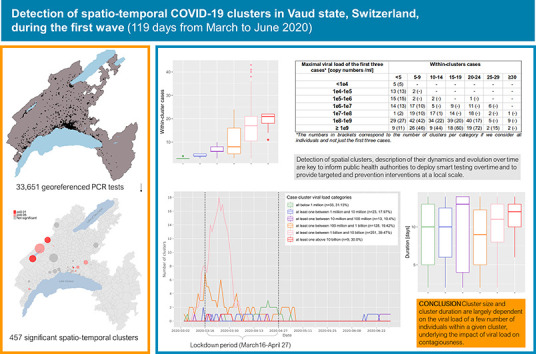
Graphical abstract

1. Introduction

The novel coronavirus SARS-CoV-2 that causes the COVID-19 disease has impacted society at an unprecedented scale. The number of infected people increased rapidly around the globe, with over 141 million confirmed cases as of April 2021 and more than 3 million deaths (World Health Organization, 2021a; World Health Organization, 2021b). The rapid dissemination of the disease has challenged international experts and policymakers to implement strategies with regards to local viral spread, healthcare resources, economic and political factors (Nicola et al., 2020; see also the cross-country analysis of COVID-19 response: https://analysis.covid19healthsystem.org/). Contact tracing, lockdowns and quarantines have been implemented around the world in a bid to contain the virus spread, and has impacted over four billion people worldwide (Chu et al., 2020). These measures are aimed at protecting approximately 22% of the world's population at risk of severe COVID-19 complications (Clark et al., 2020), with important social and economic consequences (Chu et al., 2020; Ruktanonchai et al., 2020; Faber et al., 2020).

COVID-19 outbreaks occur via close contacts, which form clusters of positive cases. Critical challenges for containing the spread of the virus lie (i) in the early detection of clusters, which reflect active viral transmission (De Ridder et al., 2020a), and (ii) in the understanding of the spatial and temporal evolution of clusters (Hohl et al., 2020). Geospatial tools using the precise location of the place of residence of tested individuals are highly effective to monitor an epidemic (Franch-Pardo et al., 2020; Keesara et al., 2020). They allow for the implementation of targeted strategies to control the local spread of disease through space and time (Cromley, 2019).

Although widely used, there is no general agreement on the definition and concepts relating to clusters, outbreaks and hotspots, particularly given a spatial context. Yet, information available from public health departments around the world converge despite existing differences. The term “cluster” generally refers to a temporal aggregation and a spatial concentration of infection cases. Generally, COVID-19 clusters are defined as two or more test-confirmed cases – though this varies to three or more in France (www.santepubliquefrance.fr) and Switzerland, up to 10 or more in New Zealand (www.health.govt.nz) – between individuals associated with a specific non-residential setting with illness onset dates within 7 to 14 days. To further label clusters as an “outbreak”, one must also have either (i) identified direct exposure between at least two of the test-confirmed cases in that setting (for example under one meter face-to-face) during the infectious period of one of the cases, or (ii) if there is no sustained local community transmission, noticed the absence of an alternative source of infection outside the setting for the initially identified positive case (Public Health England, 2020). Clusters are also assimilated to the concept of “hotspot”, which is not clearly defined neither but often used in spatial epidemiology (Lessler et al., 2017). The World Health Organization (WHO) has defined a set of methods and procedures to identify epidemic hotspots for use in global surveillance of populations (UNAIDS/WHO, 2013). Additionally, infectious diseases studies have proposed methods to identify and characterize spatial clusters (Bejon et al., 2010; Bousema et al., 2012).

The identification of high prevalence areas for any phenomenon constitutes a specific research domain in spatial statistics. Point pattern analysis (Gatrell et al., 1996) and local spatial autocorrelation methods have previously been applied in the detection of disease clusters (Jacquez and Greiling, 2003). In the current COVID-19 pandemic, Zhang et al. (2020) used local Moran's statistics to identify clusters in China at a large geographic scale using incident cases aggregated at the level of large administrative units. Among studies involving geospatial information reviewed by Franch-Pardo et al. (2020), few have characterized the spread of COVID-19 across space and time (e.g. Desjardins et al., 2020), and even fewer studies used spatial statistics to detect clusters at a local scale (De Ridder et al., 2020a; De Ridder et al., 2020b). More studies at local and regional scales that consider demographic characteristics of a population at risk are needed to provide timely information to enable accurate prevention and containment measures (Franch-Pardo et al., 2020). Indeed, the precise detection of spatial clusters, the description of their dynamics and evolution over time in a geographical context are key to inform decision-makers, to deploy smart testing overtime, and to provide targeted health and prevention interventions at a local scale (Kamel Boulos and Geraghty, 2020).

The persistence in time of clusters were shown to be associated with socio-economic deprivation (De Ridder et al., 2020b), but the size and duration of clusters are also likely to be due to “super-spreader” individuals or events (Danis et al., 2020). These super-spreader individuals or events are considered to greatly contribute to the transmission of an infectious disease (Lau et al., 2020). This process relates to the evidence for large variation in individual reproductive number, where some individuals contribute more than others to epidemics (Lloyd-Smith et al., 2005). Super-spreaders correspond to the small percentage of individuals (20%) within any population to control most (80%) transmission events (the 20/80 rule; see (Stein, 2011)). Super-spreaders are also present for the SARS-CoV-2 virus (Lau et al., 2020; Frieden and Lee, 2020); these individuals are more likely to be highly infectious, which is suggested to be related to high viral loads (Beldomenico, 2020). Notably, as recently shown in (Jacot et al., 2020), the viral load of people infected with SARS-CoV-2 appears to be similar to what is observed for other respiratory viruses such as influenza B. It remains to be explored why SARS-CoV-2 exhibits such a high reproductive number (R0) of about 2 to 3.5 (Liu et al., 2020), and if the transmission pattern, cluster duration and size somehow correlate with viral load within a detailed spatio-temporal context.

Here, we characterize the spatial and temporal dynamics of the first wave of SARS-CoV-2 infections in the state of Vaud (western Switzerland) through the detection and location of clusters. Clusters are defined by location and time where individuals are expected to have been in contact (rather than by observed contacts between individual). For each cluster, we measure size, duration and composition (number and age of individuals, as well as their viral load). We use the results of the SARS-CoV-2 RT-PCR tests (n = 33,651) performed by the Microbiology Laboratory of the Lausanne University Hospital (CHUV) between January 10 and June 30, 2020 (with a first positive case on March 2, 2020). The data used here include the results of RT-PCR tests, viral loads (copies/ml) for positive tests, individual age, and geographic location of residence for individuals tested. We used a spatial scan approach (Kulldorff, 1997; Moraga and Montes, 2011) to (i) detect spatio-temporal clusters of COVID-19 on a daily basis, (ii) disentangle the relationships between cluster size, duration and composition, and (iii) assess the importance of viral load in the evolution of clusters. We also implemented a Modified Space-Time DBSCAN (MST-DBSCAN) algorithm (Kuo et al., 2018) to characterize the diffusion dynamics of transmission clusters. Finally, we discuss the effects of a soft lockdown used across Switzerland between March 19 and April 27, 2020, on the spread dynamics of the virus.

2. Material and methods

2.1. Patients

Patients exhibiting symptoms compatible with COVID-19, including fever, cough, dyspnea, and loss of smell or taste, were tested using RT-PCR for the presence of the SARS-CoV-2 in their nasopharyngeal secretions, particularly for those considered as either vulnerable (e.g., immunosuppressed, obese, with chronic obstructive lung disease or age > 65 years) or likely to be exposed to vulnerable people (e.g. healthcare workers or those living with vulnerable persons). The studied population therefore predominantly includes vulnerable symptomatic individuals. Moreover, people who had been in contact with positive cases were also tested and included in the study, even if asymptomatic, to determine the necessity of a 10 day quarantine or isolation period. The precise residential address and age of the patient was collected at the time of sampling.

2.2. SARS-COV-2 RT-PCR

Most RT-PCR were performed using the automated molecular platform implemented at the Institute of Microbiology (Lausanne University Hospital, CHUV). It uses the Magnapure automated RNA extraction method followed by PCR amplification on QuantStudio automated systems (Greub et al., 2016) with primers described by Corman et al. (2020), later slightly modified according to Pillonel et al. (2020) to further improve PCR sensitivity. From March 24, 2020, most RT-PCR were performed with the COBAS 6800 RT-PCR test, which exhibited similar performance than the home-brew automated approach (Opota et al., 2020). Some cases (n = 71) were tested using the GeneXpert approach to reduce processing time (Moraz et al., 2020). Viral load was calculated based on the “cycle threshold” (Ct) defined as the number of cycles required for the fluorescent signal to cross a given value threshold (Opota et al., 2020; Moraz et al., 2020).

2.3. Study area

Data were collected in the south-western Swiss state of Vaud, north of Lake Geneva. Vaud has an area of 3212 km² (Fig. 6A) with a population of 811,203 (end of 2019), giving an average density of 249 inhabitants/km². Notably there are population density differences between the urban area of Lausanne-Morges on the shores of Lake Geneva (~3000 inhabitants/km²) and rural areas towards the north (~200 inhabitants/km²). An exception is the area of Yverdon-les-Bains, located directly south of the Lake of Neuchâtel with ~2200 inhabitants/km².

Fig. 6.

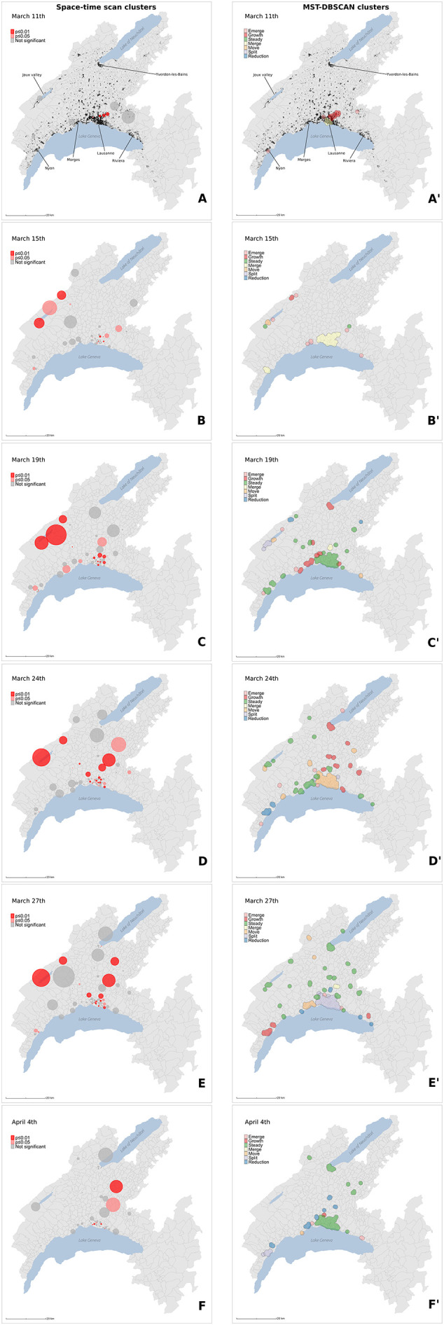
Spatial distribution of case clusters (A-F) and diffusion dynamics of transmission clusters (A′–F′) for 6 key dates (March 11, March 15, March 19, March 24, March 27, April 4) during the first epidemic wave. Case clusters resulting from the prospective Poisson space-time scan statistics (A–F) are shaded according to their significance level: dark red for statistically significant clusters with alpha = 0.01, light red for statistically significant clusters with alpha = 0.05, and grey for non-significant clusters (p > 0.05). Transmission clusters resulting from the MST-DBSCAN algorithm (A′–F′) are shaded according to their evolution type: emerge (pink), growth (red), steady (green), merge (yellow), move (orange), split (purple), and reduction (blue). Black points in (A) and (A′) represent the 33,651 individuals tested during the study period (January 10 to June 30). (For interpretation of the references to color in this figure legend, the reader is referred to the web version of this article.)

2.4. Spatio-temporal clusters

We used SaTScan software (version 9.6.1) to detect daily space-time clusters of individuals who were tested positive for SARS-COV-2 in the state of Vaud from March 2 to June 30, 2020, (no positive cases between January 10 and March 2, 2020). The algorithm developed by Kulldorff (1997) tests whether a disease is uniformly distributed among individuals over space and time. It uses a “moving cylinder”, with the base and height corresponding to the spatial and temporal components, respectively. Significance tests evaluate excess relative risk, i.e., more observed COVID-19 cases than expected within the moving cylinder relative to randomly distributed cases over space and time. We implemented this algorithm across a daily prospective surveillance analysis. We used a discrete Poisson model, where the number of events in the geographic area (total number of positive tests) is Poisson-distributed, according to a known underlying population at risk. Though typical SaTScan applications use the default value of 50% of the population at risk for the spatial size cluster's radius, here we selected a radius covering a maximum of 0.5% of the total resident population (population at risk) in the state of Vaud (N = 811,203 inhabitants; SFSO, 2019), as a smaller value emphasizes the discovery of small and homogeneous clusters (Chen et al., 2008). Tested individuals and the underlying population at risk were georeferenced at the centroids of a hectometric grid (SFSO, 2020) covering the entire study area. The minimum number of positive cases considered to constitute a cluster was set to three, and we restricted the temporal scanning window to a minimum of two days and a maximum of 14 days (see Supp. Mat. 1). The upper limit of 14 days accounts for the incubation period (generally 2 to 7 days) and infectious time (generally 7 to 10 days from symptom onset, as deduced from different culture-based and RT-PCR-based investigations; Jaafar et al., 2020; Jeong et al., 2020; Caruana et al., 2021; To et al., 2020). The significance of the clusters was evaluated on the basis of 999 Monte-Carlo permutations that randomized both locations (Besag and Diggle, 1977) and times of the cases.

2.5. Cluster evolution and diffusion zones

We used MST-DBSCAN (modified space–time density-based spatial clustering of application with noise; Kuo et al., 2018) to characterize the diffusion dynamics of clusters. MST-DBSCAN is an algorithm used to detect, characterize, and visualize disease cluster evolution in geographic space and time. It geographically computes a kernel density that considers the effect of the incubation period of an infectious disease. It is based on DBSCAN (Ester et al., 1996), a non-parametric density-based clustering algorithm that groups together objects (here, SARS-COV-2 positive cases) that are closely packed together (points with many nearby neighbors), marking points falling in low-density regions as outliers. The MST-DBSCAN identifies seven different cluster behaviors: a) emerge, b) grow, c) remain steady, d) merge, e) move, f) split or g) reduce.

We applied the MST-DBSCAN analysis to the 3317 COVID-19 positive cases identified (among 33,651 tested individuals), georeferenced at their precise residential address in the state of Vaud. Disease clusters were computed daily from March 4, 2020, to June 30, 2020. The maximum spatial radius considered was 1000 m, with a time window of 1 to 7 days to reflect the average infectious period after a positive test (see Supp. Mat. 1). A cluster was defined as a minimum of three positive cases. For all identified clusters, we established a typology of similar diffusion patterns in the geographical space. We associated clusters with postcodes areas (557 units; MicroGIS, 2019) in the state of Vaud to use as spatial references. Then, we focused on three main behaviors to characterize the diffusion type through the postcode areas: a) Increase, if an area was covered by clusters whose evolution type was Emerge, Growth, or Merge; b) Keep, if an area was covered by clusters whose evolution type was Steady or Move; c) Decrease, if an area was covered by clusters whose evolution type was Reduction or Split. Postcodes with similar diffusion patterns over the entire study period were grouped using the Louvain method, a group detection algorithm that uses network analysis (Blondel et al., 2008). This approach synthetizes the spatio-temporal information and facilitates its visualization on a single map. Equations for the MST-DBSCAN approach are provided in Supp. Mat. 2.

3. Results

3.1. Epidemic trajectories of positive cases

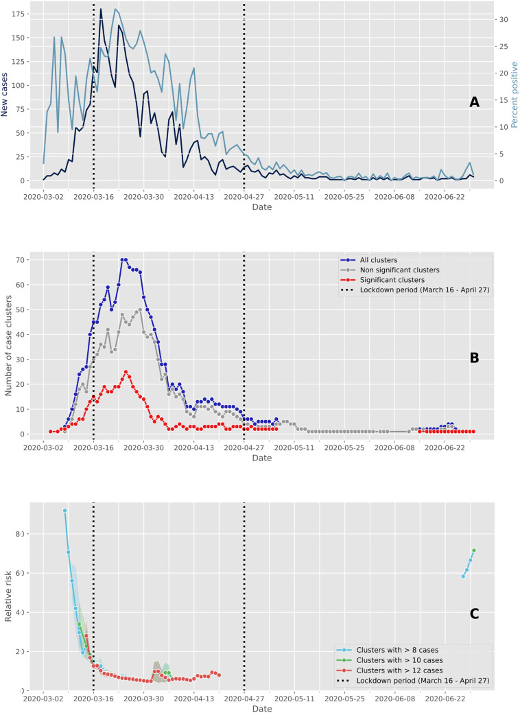
A total of 33,651 individuals were tested over a period of 6 months (March 2 to June 30, 2020), of which 3317 (9.86%) were confirmed as positive using RT-PCR. Of these positive cases, 79% (2609/3317) occurred between March 9 and April 5, though this four week period corresponds to only 16% of the study period total duration (Fig. 1A). The peak of the first epidemic wave occurred on March 18, which was two days after the soft lockdown was implemented in Switzerland, that lasted from March 16 to April 27 (vertical dashed lines in Fig. 1A). Up to 180 individuals a day were documented as “positive” in our laboratory at the peak number of cases during the study period (Fig. 1A, dark blue). The number of positive cases then decreased considerably from the first of May. The highest proportion of positive tests was observed four days after the peak of the epidemic wave, with a rate of positive tests reaching 32% (Fig. 1A, light blue). The rate of positive cases was relatively high at the start of the epidemic when few individuals were tested. After this, the shape of the curve of the percentage of positive tests followed the one of the number of cases. This is likely because at the beginning of the epidemic, only individuals with symptoms and those at risk were tested, and it was only later that a much wider range of individuals were tested such that all symptomatic individuals and asymptomatic individuals in contact could access a test.

Fig. 1.

Evolution of cases and clusters through time. The vertical dashed lines delimit the Swiss lockdown period (March 16 to April 27). (A) Epidemic trajectory of positive tests. The daily new confirmed cases are represented in dark blue and the percent of positive tests are represented in light blue. (B) Number of case clusters over time. The total number of clusters detected daily by space-time scan statistics are represented in dark blue, and the red and grey lines represent the proportion of significant clusters (p ≤ 0.05) and non-significant clusters (p > 0.05), respectively. (C) Average relative risk of significant space-time clusters (p ≤ 0.05) over time according to within-cluster cases. (For interpretation of the references to color in this figure legend, the reader is referred to the web version of this article.)

3.2. Cluster detection and temporal dynamics

We identified 1684 space-time clusters of more than two cases using residential address for individuals tested positive to SARS-CoV-2. Of these, 457 clusters were considered significant based on the within-proportion of positive cases compared to the total documented positive cases. Highest values of both significant and non-significant clusters were observed between March 9 and April 5 (Fig. 1B) and then the number of clusters decreased. The decrease in positive cases following the beginning of the soft lockdown (Fig. 1A) occurred approximately two weeks before the decrease in the number of clusters (Fig. 1B). The number of clusters displays a similar pattern through time but with a difference in amplitude. As shown in Fig. 1C, the estimated relative risk for new clusters was greater before the soft lockdown and approximately 80 days after the end of the lockdown. The size of the clusters (i.e., number of cases within clusters) used to compute the relative risk did not strongly change the value of the relative risk during the core of the epidemic wave. However, cluster size affected relative risk when the number of positive cases was small, such as at the beginning and at the end of the epidemic wave.

3.3. Cluster composition

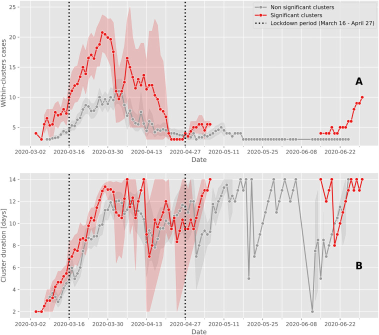
Significant space-time clusters generally involved a larger number of positive cases (maximum mean of 21 cases, where the largest cluster had 43 cases on March 25) compared to non-significant clusters (maximum mean of 11 positive cases; Fig. 2A). Notably, significant clusters with more than 15 positive cases were predominantly observed shortly after the soft lockdown was implemented from March 16 to April 27, with one exception on April 3 (Fig. 2A). Cluster durations – although limited to 14 days - increased over time from the start of the epidemic wave, showing little differences between significant and non-significant clusters. There was an absence of significant clusters from May 3 to June 16 (Fig. 2B).

Fig. 2.

Case cluster characteristics over time.

The mean and confidence intervals of the number of cases within clusters (A) and the duration of clusters (B) are calculated for significant (red line) and non-significant clusters (grey line). Between May 6 and June 15, the prospective space-time scan statistic detected no significant clusters. The vertical dashed lines delimit the Swiss lockdown period (March 16 to April 27). (For interpretation of the references to color in this figure legend, the reader is referred to the web version of this article.)

3.4. Viral load in clusters

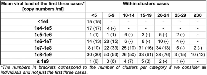
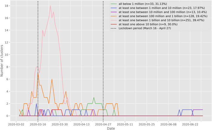
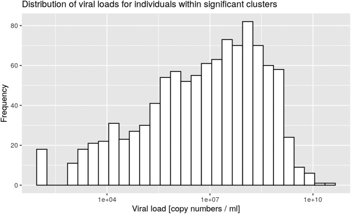
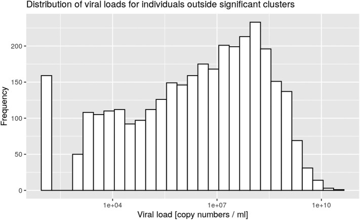
Clusters were defined by the presence of at least three positive cases within a limited geographic area, as documented in the SaTScan analysis. All clusters were then characterized according to the nasopharyngeal viral load of the cases for each cluster (Table 1). Five significant clusters were composed of three cases exhibiting a viral load below 10,000 copies/ml at time of testing, which is the same low load as found in non-significant clusters (Supp. Mat. 5). However, significant clusters were more likely to be detected when viral loads were above 100 million copies/ml (Fig. 3). Finally 18 significant clusters with at least one individual showing between 1 billion and 10 billion copies/ml were documented on March 24 (Fig. 3, pink curve). There was a significant difference between the frequency distribution of viral loads in significant clusters compared with non-significant clusters and outside clusters (Kolmogorov–Smirnov test, two-sample case, p < 0.001, see Supp. Mat. 3, Supp. Mat. 4).

Table 1.

Classification of the space-time clusters according to the viral load of the cases involved. Within-cluster cases were identified by matching both geographically and temporally positive test subjects, geocoded at the residential address, with space-time clusters. For example, a cluster was classified as “all below 1 million” if all individuals tested positive within the cluster during its active period had a viral load below 1 million copies/ml.

For each cluster category, the total number of case clusters detected by prospective space-time scan statistics over the entire study period (March 2 to June 20) and the proportion of significant clusters (p ≤ 0.05) are reported.

Case cluster viral load category	Total number of clusters	Number of significant clusters
All below 1 million	106	33 (31.1%)
At least one between 1 million and 10 million	128	23 (17.9%)
At least one between 10 million and 100 million	125	13 (10.4%)
At least one between 100 million and 1 billion	659	128 (19.4%)
At least one between 1 billion and 10 billion	636	251 (39.4%)
At least one above 10 billion	30	9 (30.0%)
Total	1684	457

Supp. Mat. 5.

Mean viral load of the first three cases within clusters

Fig. 3.

Number of significant (p ≤ 0.05) case clusters over time characterized according to the viral load of the cases documented in each cluster. The vertical dashed lines delimit the Swiss lockdown period (March 16 to April 27). For each cluster, we extracted the positive test individuals intersecting the cluster both geographically and temporally, and we characterized the clusters according to the viral load of the individuals composing it. The clusters represented in green are composed only of individuals with a viral load of less than 1 million copies/ml. The clusters shown in blue are made up of at least one individual with a viral load between 1 million and 10 million copies/ml, and so on. (For interpretation of the references to color in this figure legend, the reader is referred to the web version of this article.)

Supp. Mat. 3.

Distribution of viral loads for individuals within significant clusters

Supp. Mat. 4.

Distribution of viral loads for individuals outside significant clusters

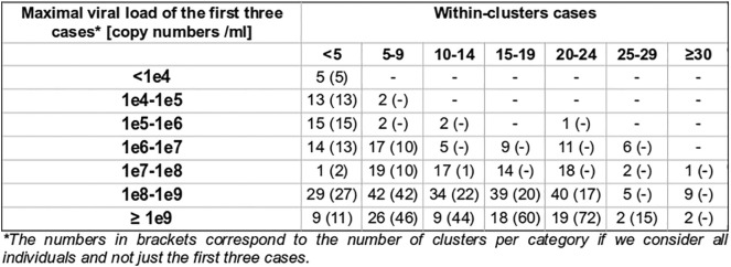
The mean viral load of the first three cases was also studied, in order to gain insight of the possible relationship between nasopharyngeal viral load and contagiousness, indirectly measured by the documentation of subsequent clusters. For 20 significant clusters, all first three cases exhibited a viral load below 100,000 copies/ml, suggesting that individuals with fewer than 100,000 copies/ml may still be contagious (Supp. Mat. 6). Moreover, the nasopharyngeal viral load of the first three cases was below 1 million copies for 40 significant clusters.

Supp. Mat. 6.

Maximal viral load of the first three cases within clusters

3.5. Cluster size, duration and viral load

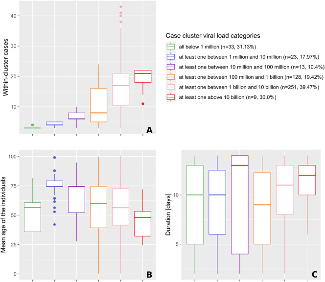
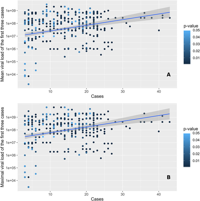
Cluster size was positively associated with the presence of individuals with high viral loads (Fig. 4A). The highest viral loads measured were greater than 10 billion copies/ml and occurred in the largest clusters (median of 21 positive cases). This was used to identify super-spreading events. When comparing clusters harboring individuals with all viral loads below 1 million copies/ml with the ones where at least one case had a viral load above 1 million copies/ml, the cluster sizes were significantly different, with median cases per cluster increasing from three to four (p < 0.001; Fig. 4A). Similar relationships were observed when considering the mean and maximal values of viral loads of the first three positive cases (Fig. 5A & B).

Fig. 4.

Characteristics (size, age and duration) of significant space-time clusters (p ≤ 0.05) over the study period, categorized according to the viral load of the cases involved.

The classification procedure is explained in more details in the legend of Table 1. Characteristics include the number of cases observed in clusters (A), the mean age of the positive tests individuals forming clusters (B), and the duration of clusters (C).

Fig. 5.

Number of cases observed within significant space-time clusters (p ≤ 0.05) in function of the mean (A) and maximal (B) viral loads of the first three cases involved. Points are colored according to the significance level of the cluster, as assessed through 999 Monte Carlo random permutations.

Highest viral loads were found in clusters with individuals showing the lowest average age group considered in the investigation. Clusters composed of individuals in the highest average age group showed low to middle viral loads (Fig. 4B). The median age of individuals within a cluster was significantly higher when the cluster viral load was between 1 and 10 million copies/ml. The average age group then progressively decreased from 74 to 48 years, while viral load increased. Cluster duration was only significantly different between the orange category (100 million to 1 billion/ml) and the pink category (1 to 10 billion/ml), where clusters of the latter lasted half a day longer (mean of +0.46 days, p < 0.001; see Fig. 4C).

Clusters with individuals in the lowest average age group considered in the investigation and clusters with the highest viral loads (Fig. 4B) also constitute the largest clusters (Fig. 4A) and those that last the longest (Fig. 4C), respectively.

3.6. Geographic distribution of the first epidemic wave

We chose six key dates to illustrate the evolution of the two cluster types during the first wave of the epidemic in the state of Vaud. Animations showing the spatio-temporal evolution of the clusters for the entirety of the first wave and showing the dynamics of clusters' behavior can be found in Supp. Mat. 7 and Supp. Mat. 8, respectively. Fig. 6 shows the spatial distribution of space-time clusters (A–F) and compares it to information translating the diffusion dynamics of the clusters (A′–F′). A detailed description of the first SARS-CoV-2 epidemic wave in the of Vaud can be found in Box 1, illustrating the powerful and critical information that the approach offers.

Box 1. The first SARS-CoV-2 epidemic wave in the state of Vaud, Switzerland.

On March 11, 2020, 7 days after the first detection of a positive case (Fig. 6A), we observe a phase of rapid growth and merging (see Fig. 6A′), where a series of significant clusters appear directly north of Lausanne, the main city of the state. Interestingly, three out of the four clusters shown are located in wealthy areas. March 15 (Fig. 6B and B′) is the day before the soft-lockdown. There are multiple clusters in the Lausanne area, among which a large fraction are significant (Fig. 6B). Fig. 6B′ shows that these clusters rapidly merged into a single “super cluster” deployed over the urban agglomeration. In the rural areas, active clusters emerge and grow north of the lake in the Joux valley, located in the Jura mountains, where population density is low. Four days later, on March 19 (Fig. 6C and C′), the peak of the first wave is approaching (see Fig. 1B). The number of case clusters is high in the Lausanne area (Fig. 6C) but stabilizes. Similar behavior is observed towards the east along Lake Geneva; only one moving cluster is observed in the Riviera area (Fig. 6C′), compared with new clusters appearing in the Morges area to the west. In the Joux valley, the activity remains important, and a cluster grows in Yverdon-les-Bains, south of the Lake of Neuchâtel. On March 24 (Fig. 6D and D′), the peak of the first wave is reached (see Fig. 1B). New cases reactivate moving clusters in the center of Lausanne, while towards west the situation stabilizes and even reduces towards Geneva with no further significant cluster in the Nyon area. At the peak, a large significant cluster remains steady in the Jura, and several clusters grow in the remote, rural periphery north of the main urban area (Fig. 6D and D′). In the north, close to the Lake of Neuchâtel, the clusters are not significant despite growing. On March 27 (Fig. 6E and E′), all clusters start an important and rapid reduction phase (see Fig. 1B). The merged clusters of the Lausanne area split, and most clusters in the country-side remain steady. However, a significant cluster emerges in the west, in the Nyon area. On April 4 (Fig. 6F and F′), the peak ends. The Joux valley cluster ends after 25 days and clusters in the state are either no longer significant, or are steady, split of reduce. There is one exception north of Lausanne with a single growing cluster located in a leisure area and is likely related to the presence of a school (with boarding).

Alt-text: Box 1

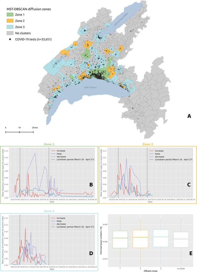
Cluster behaviors described in Box 1 were summarized with four diffusion zones shown in Fig. 7A and identified at the level of postal code areas using MST-DBSCAN (Fig. 7B, C, D). The grey diffusion zone corresponds to areas where no clusters emerged, while the green, orange and blue diffusion zones differ in the way clusters evolved over time. The green diffusion zones correspond to areas where the clusters immediately increased in size at the beginning of the epidemic wave (red line, Fig. 7B), but decreased drastically once the soft lockdown (vertical dash line) was implemented. We then observed a second peak associated with an important increase of clusters that reduced in size (red line, Fig. 7B). Both red and purple curves are bimodal and tended to decrease afterwards, with a few numbers of new small peaks that plateau forming a distribution with a long right tail. Conversely, orange and blue diffusion zones show a first peak of increasing clusters later, at about the time of the start of the soft lockdown (orange & blue areas, Fig. 7C and D). Both zones also show clusters that remained stable in size during the soft lockdown (blue line). Only the blue diffusion zone showed no further clusters after April 27, which corresponds with the end of the lockdown, and is the only zone that did not display a bimodal distribution of clusters. Note that no difference in viral load was documented among these different diffusion zones (Fig. 7E).

Fig. 7.

(A) Diffusion zones identified by the MST-DBSCAN algorithm. Postcode areas with the same color share similar diffusion patterns, and areas without any transmission clusters are represented in grey. The black dots on the map indicate the 33,651 individuals tested for COVID-19 in the state of Vaud between January 10 and June 30, 2020. Below the map are the frequencies of major evolution types over time for zone 1 (B), zone 2 (C) and zone 3 (D). The red line corresponds to the “increase” diffusion type whose area grows with time, the blue line corresponds to the “keep” diffusion type assigned to clusters whose area remains stable, and the purple line corresponds to the “decrease” diffusion type whose area becomes smaller. The vertical dashed lines delimit the Swiss lockdown period (March 16 to April 27). (E) Distribution of the viral load of test-confirmed cases living in each diffusion zone. (For interpretation of the references to color in this figure legend, the reader is referred to the web version of this article.)

4. Discussion

The discussion is divided into three major parts. The first highlights results that uncover new information on COVID-19 clusters, the second summarizes limitations of the interpretation of the results, and the third describes the added value of these methods for tackling epidemic problems and evaluating the effects of lockdown strategies.

4.1. New information on COVID-19 clusters

4.1.1. A temporal lag between documentation of positive cases and clusters burden

Significant clusters were predominantly observed from March 15 to April 5 (red curve in Fig. 1B), while non-significant clusters in high population-density areas, such as Lausanne, were documented 4 to 5 days earlier and continuously occurred until mid-May (grey curve on Figs. 1B, and 6A). We observed a time-shift between the decrease in the number of positive cases and the decrease in the number of clusters. This delay could be explained by the fact that most positive cases might have been at the origin of lasting clusters, i.e. clusters that last longer than 10 days from when their first positive cases are identified. Interestingly, the number of patients hospitalized at Lausanne University Hospital (CHUV) and the number of COVID-19-related deaths in the state of Vaud also followed the same epidemic curve, but with a two weeks delay (personal communication, G. Greub).

4.1.2. Viral load is strongly informative about the presence and size of SARS-CoV-2 clusters

Our results show that clusters at the peak of the SARS-CoV-2 epidemic wave were composed of individuals with a high viral load. Cluster size is positively associated with the presence of individuals with a high viral load in significant clusters, though in 40 clusters the first three cases exhibited a viral load below 1 million copies/ml, including 33 clusters with individuals that had a nasopharyngeal viral load below 1 million copies/ml. Moreover, as many as 20 clusters were composed of cases that initially had a viral load below 100,000 copies/ml, suggesting that subjects with fewer than 100,000 copies/ml may still have been contagious.

The fact that significant clusters are composed of patients with viral loads as low as those found in non-significant clusters further supports the hypothesis that community transmission can occur with low levels of viral load. Nevertheless, this may also reflect a statistical bias as large clusters with more than 10 individuals are more likely to have at least one individual with a very high viral load.

4.1.3. Advantage of RT-PCRs over antigen-based testing

Given the relatively low sensitivity of antigen tests, we estimate that we would have missed or had delayed identification of approximately 24 clusters. Indeed, the 20 significant clusters with a viral load of the three first cases below 100,000 copies/ml would not have been detected with antigen tests, given that the best tests have a detection limit of about 100 to 200,000 copies/ml (Caruana et al., 2021). Moreover, the clusters with a case between 100,000 copies/ml and 1 million copies/ml would not have been detected in 5% of cases given an overall antigen sensitivity for such viral load of about 80% (Caruana et al., 2021). Thus, an antigen-based strategy would have missed about 5% (24/457) of the significant clusters. Therefore, for the second wave that began in October 2020 across western Switzerland, we advocated against the use of antigen tests for the vulnerable population and healthcare workers, as well as with non-vulnerable subjects during non-acute periods of SARS-CoV-2 infection (1 to 4 days of symptoms), despite encouraging results for antigen tests in subjects within the first four days of symptom onset (Schwob et al., 2020).

4.1.4. High viral load in large clusters within the youngest group age

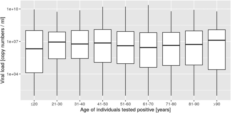
Within clusters, we found a clear negative relationship between age and level of viral load (Fig. 4B), and between cluster size and viral load (Fig. 4A). Indeed, while a high viral load was found in large clusters with the youngest group age considered in this study, low to intermediate viral load was measured in small clusters composed of older age groups. This suggests that large clusters were generated by active individuals from the working population, and super-spreader events may be at the origin of such large clusters. Surprisingly, when the level of viral load was analyzed across age groups, no relationship was found (Supp. Mat. 9), meaning that useful information emerges within clusters. Indeed, the characterization of the clusters provides a deeper analysis of the mechanisms behind the progression of an epidemic and the geographic analysis of clusters of cases might constitute a type of investigations to favor in the future.

Supp. Mat. 9.

Boxplots of viral load per age class of individuals tested positive

4.1.5. Non-significant clusters also convey information on the progression of the epidemic

Significant and non-significant clusters both show the same epidemiological trajectories. Indeed, they display similar patterns in terms of changes in size, differing only in amplitude. This suggests that the occurrence of clusters, even if non-significant, is a good estimator of the epidemic situation. Significant and non-significant clusters differ in terms of number of cases and measured viral load, but not in duration. This suggests that non-significant clusters (i) might correspond to transmission events unrelated to subjects with very high viral load, (ii) translate a lower impact on the population in terms of viral spread, and (iii) express a transition towards or from a significant spatio-temporal configuration.

4.2. Limitations

4.2.1. Tested population is not homogeneous through time

During the course of the studied epidemic wave, recommendations for testing as requested by the authorities changed. Initially, only symptomatic patients at risk and health workers were tested. Then, from mid-March a wider proportion of the population was progressively tested, though younger individuals still were reluctant to get tested. This may have generated heterogeneity in our longitudinal investigation. Moreover, tests were likely performed at different stages of infection (early, late, etc.) and might not be representative of the correct window of infection. The day of the week may also have generated differences in the number of positive tests. Indeed the number of tests was often smaller during weekends, as some individuals preferred being tested only on the following Monday to avoid quarantining over the weekend.

4.2.2. Positive cases might be missing

Our estimate of the number of positive cases is not fully representative of the epidemic, particularly at the beginning when only symptomatic at-risk patients and health workers were tested. We might expect that close relatives of positive cases were also infected but not tested due to reagent shortage. However, this bias might have a limited impact on the assessment of cluster size, as any person in contact with a positive case (documented by the contact tracing team) was tested. An additional source of underestimation could be from the false negative RT-PCRs results due to imperfect nasopharyngeal sampling, though the clinical sensitivity of RT-PCR performed on nasopharyngeal samples in our laboratory is very sensitive, with 96 to 98% accuracy (Schwob et al., 2020; Mueller et al., 2020). Similarly, the rate of false positives in the same laboratory was estimated to be lower than 1/10,000 tests, due to full automation and bar-coding that was used to prevent human error and samples/tubes inversion (Greub et al., 2016). Asymptomatic patients might also contribute to the spread of the disease, though those individuals were not detected and thus could not be accounted for in this study unless they were among the contacts traced from positive cases. Finally, missing positive cases could be from people living or working at the state border, such that they were tested elsewhere. However, this seems to have a limited impact as over 80% of all samples tested for SARS-CoV-2 in 2020 were obtained from individuals living in the state of Vaud.

4.2.3. Many space-time scan clusters

In this study, we adopted a posture to reproduce the daily monitoring of the epidemic. As a result, the analysis was repeated each day. In this configuration the number of clusters detected is unusually high compared to the total number of positive cases. Indeed, the same subset of positive cases can be responsible for several clusters if an area presents an excessive relative risk for several days in a row, as we consider a time window of 14 days. This is why the clusters' summary statistics for viral load, cluster's duration, and age of the subjects is smoothed.

4.3. Added value of the methods used

4.3.1. Geographic clusters to characterize epidemics: a key tool for intervention

Despite the lack of a formal definition for clusters in a geographical context, the statistical approaches used here make implicit assumptions that – through different parameters – have a direct influence on cluster detection and interpretation. We used two complementary approaches that highlight different key aspects of disease clustering. Space-time scan statistics detect the geographical location of case clusters, assess their significance, and characterize their relative risk and duration. This prospective approach is particularly appropriate for the establishment of a daily surveillance system, as it identifies ‘alive’ clusters only, i.e. having an excess of relative risk on the day of analysis (Kulldorff, 2001). Unlike other detection methods, this approach searches for clusters without imposing the specification of their size and allows for the analysis of areas with heterogeneous population densities. Indeed, it identifies a cluster if the risk of disease within a space-time cylinder (radius = space, and height = time) is higher than outside the cluster. This information is key for public health authorities to target neighborhoods and calibrate protective or preventive measures to be deployed.

The MST-DBSCAN algorithm characterizes the diffusion dynamic of the epidemic. Here, the input parameters require a precise definition of the incubation period, the cluster transmission areas, and a minimum number of spatio-temporal neighbors required to form a cluster (Kuo et al., 2018). The algorithm returns a typology of the evolution of transmission clusters, and identifies administrative units that are undergoing a similar diffusion process. Compared to space-time scan statistics, the MST-DBSCAN algorithm explicitly considers transmission relationships between cases but does not provide information about the cluster size (i.e., the within-number of cases) nor its statistical significance. The two approaches used together therefore allow for detailed monitoring of the disease's epidemic trajectory and populations at risk, and offer adequate tools for governments to both prioritize interventions on excess-risk locations and to develop adapted strategies to control cluster diffusion types.

4.3.2. Maps reflect the chronology of the epidemic

The results displayed on static and animated maps reflect the chronology of the sanitary situation during the first wave of the epidemic. For instance, the major clusters in the Joux valley area can be clearly observed on different maps (Fig. 6B, B′, C, C′). Notably, these large clusters originate from a super-spreader event that took place at the end of February in a religious ceremony in Mulhouse, France. Many Swiss residents participated in this ceremony, and related clusters were then observed during the same period north of the Lausanne urban area and along the Jura mountains (e.g., in Morges and Nyon). Conversely, Lausanne was hit early-on by clusters, which is likely due to a first transmission event that occurred in Northern Italy.

Interestingly, the initial phase observed in the state of Vaud differs from what happened in Geneva, where the first clusters emerged in deprived neighborhoods eight days (March 5) after the first positive case (February 26) was detected (De Ridder et al., 2020a; De Ridder et al., 2020b). In Vaud, however, the initial cluster was directly detected the day of the first cases (March 4), with nine positive results in a wealthy neighborhood.

4.3.3. Positive impact of soft lockdown

The soft lockdown was directly associated with a rapid reduction in the number of positive cases despite the increased rate of testing. This important reduction takes place in two clear phases in the main urban areas (see Fig. 7B), while the reduction of positive cases occurs as a succession of clusters increase and decrease in smaller urban centers and less dense areas (Fig. 7D). However, due to the time lag between the identification of positive individuals and the constitution of clusters, the cluster burden occurred directly after the implementation of the soft lockdown. Similarly, the largest clusters, the longest duration and the clusters with individuals showing large viral loads were observed just after the same time-lag. This time lag appears to be shorter in urban areas than in rural areas, likely reflecting the faster spread of the virus in large towns such as Lausanne, Morges, Nyon, Yverdon and along the Vaud Riviera. This faster spread is likely due to differences in social and cultural organization between rural and urban areas, including denser housing, which puts a higher risk of subsequent infection in families with lower socio-economic situations.

Our results highlight the efficacy of this soft lockdown strategy in controlling the epidemic and decreasing the number of positive cases. It also demonstrates the importance of acting quickly when the number of positive cases increases and not waiting for the settlement of clusters. Additionally, our results show that the relative risk remained very low throughout the lockdown period. Of note, the compliance of Swiss residents during the first soft lockdown is signaled by the absence of any significant cluster from May 3 to June 16. Finally, it has not escaped our notice that it is already possible to observe the beginnings of the second wave from June 22, 2020 (Fig. 2A), which occurred exactly two weeks after a series of relaxations to the protective measures, including the authorization of public demonstrations of up to 300 people and the opening of nightclubs (June 6, 2020).

5. Conclusion

Our results highlight that cluster size is positively related to the presence of individuals with high viral loads, the latter being more commonly found in clusters harboring the youngest age group investigated in this study. This work also stresses the fact that cluster size and cluster duration are largely dependent on the viral load of a few number of individuals within a given cluster, underlying the impact of viral load on contagiousness.

Altogether, we provide robust data suggesting that transmission may occur despite source cases in a cluster presenting a viral load below 100,000 copies/ml. Such low viral load cases remain undetected by antigen testing, highlighting the importance of RT-PCRs assays in detecting cases and defining subsequent tracing strategies. This in-depth analysis suggests that even older at-risk individuals might get infected by SARS-CoV-2 despite active prevention, even if all cluster individuals exhibit a low viral load (below 100,000 copies/ml).

Finally, such a spatio-temporal characterization of clusters demonstrates the huge effect of the soft lockdown that took place in Switzerland from March 16 to April 27, 2020. These important results have been documented due to the contribution of the geospatial analysis of clusters.

The following are the supplementary data related to this article.

Supp. Mat. 1

Definition of time windows with SaTScan and MST-DBSCAN

Supp. Mat. 2

Main stages of the MST-DBSCAN algorithm

Supp. Mat. 7

Animated map showing the spatio-temporal evolution of the clusters during the first wave in the Vaud State

Supp. Mat. 8

Animated map showing the dynamics of clusters’ behavior during the first wave in the Vaud State

CRediT authorship contribution statement

Anaïs Ladoy: Investigation, Data curation, Methodology, Formal analysis, Software, Writing – review & editing. Onya Opota: Writing – review & editing, Resources, Validation. Pierre-Nicolas Carron: Resources, Writing – review & editing, Validation. Idris Guessous: Validation, Writing – review & editing. Séverine Vuilleumier: Writing – original draft, Writing – review & editing, Supervision. Stéphane Joost: Conceptualization, Writing – original draft, Validation, Writing – review & editing, Supervision. Gilbert Greub: Conceptualization, Writing – original draft, Validation, Writing – review & editing, Supervision.

Declaration of competing interest

The authors declare that they have no known competing financial interests or personal relationships that could have appeared to influence the work reported in this paper.

Editor: Jay Gan

References

- Bejon P., Williams T.N., Liljander A., Noor A.M., Wambua J., Ogada E., Olotu A., Osier F.H.A., Hay S.I., Färnert A., Marsh K. Stable and unstable malaria hotspots in longitudinal cohort studies in Kenya. PLoS Med. 2010;7 doi: 10.1371/journal.pmed.1000304. [DOI] [PMC free article] [PubMed] [Google Scholar]
- Beldomenico P.M. Do superspreaders generate new superspreaders? A hypothesis to explain the propagation pattern of COVID-19. Int. J. Infect. Dis. 2020;96:461–463. doi: 10.1016/j.ijid.2020.05.025. [DOI] [PMC free article] [PubMed] [Google Scholar]
- Besag J., Diggle P.J. Simple Monte Carlo tests for spatial pattern. J. R. Stat. Soc. Ser. C Appl. Stat. 1977;26:327–333. [Google Scholar]
- Blondel V.D., Guillaume J.-L., Lambiotte R., Lefebvre E. Fast unfolding of communities in large networks. J. Stat. Mech. Theory Exp. 2008;2008 [Google Scholar]
- Bousema T., Griffin J.T., Sauerwein R.W., Smith D.L., Churcher T.S., Takken W., Ghani A., Drakeley C., Gosling R. Hitting hotspots: spatial targeting of malaria for control and elimination. PLoS Med. 2012;9 doi: 10.1371/journal.pmed.1001165. [DOI] [PMC free article] [PubMed] [Google Scholar]
- Caruana G., Croxatto A., Kampouri E., Kritikos A., Opota O., Foerster M., Brouillet R., Senn L., Lienhard R., Egli A., Pantaleo G., Carron P.-N., Greub G. Implementing SARS-CoV-2 rapid antigen testing in the emergency ward of a Swiss University Hospital: the INCREASE study. 4. Microorganisms. 2021;9:798. doi: 10.3390/microorganisms9040798. [DOI] [PMC free article] [PubMed] [Google Scholar]
- Chen J., Roth R.E., Naito A.T., Lengerich E.J., MacEachren A.M. Geovisual analytics to enhance spatial scan statistic interpretation: an analysis of U.S. cervical cancer mortality. Int. J. Health Geogr. 2008;7:57. doi: 10.1186/1476-072X-7-57. [DOI] [PMC free article] [PubMed] [Google Scholar]
- Chu I.Y.-H., Alam P., Larson H.J., Lin L. Social consequences of mass quarantine during epidemics: a systematic review with implications for the COVID-19 response. J. Travel Med. 2020;27 doi: 10.1093/jtm/taaa192. [DOI] [PMC free article] [PubMed] [Google Scholar]
- Clark A., Jit M., Warren-Gash C., Guthrie B., Wang H.H.X., Mercer S.W., Sanderson C., McKee M., Troeger C., Ong K.L., Checchi F., Perel P., Joseph S., Gibbs H.P., Banerjee A., Eggo R.M., Nightingale E.S., O’Reilly K., Jombart T., Edmunds W.J., Rosello A., Sun F.Y., Atkins K.E., Bosse N.I., Clifford S., Russell T.W., Deol A.K., Liu Y., Procter S.R., Leclerc Q.J., Medley G., Knight G., Munday J.D., Kucharski A.J., Pearson C.A.B., Klepac P., Prem K., Houben R.M.G.J., Endo A., Flasche S., Davies N.G., Diamond C., van Zandvoort K., Funk S., Auzenbergs M., Rees E.M., Tully D.C., Emery J.C., Quilty B.J., Abbott S., Villabona-Arenas C.J., Hué S., Hellewell J., Gimma A., Jarvis C.I. Global, regional, and national estimates of the population at increased risk of severe COVID-19 due to underlying health conditions in 2020: a modelling study. Lancet Glob. Health. 2020;8:e1003–e1017. doi: 10.1016/S2214-109X(20)30264-3. [DOI] [PMC free article] [PubMed] [Google Scholar]
- Corman V.M., Landt O., Kaiser M., Molenkamp R., Meijer A., Chu D.K., Bleicker T., Brünink S., Schneider J., Schmidt M.L., Mulders D.G., Haagmans B.L., Veer B. van der, Brink S. van den, Wijsman L., Goderski G., Romette J.-L., Ellis J., Zambon M., Peiris M., Goossens H., Reusken C., Koopmans M.P., Drosten C. Detection of 2019 novel coronavirus (2019-nCoV) by real-time RT-PCR. Eurosurveillance. 2020;25:2000045. doi: 10.2807/1560-7917.ES.2020.25.3.2000045. [DOI] [PMC free article] [PubMed] [Google Scholar]
- Cromley E.K. Using GIS to address epidemiologic research questions. Curr. Epidemiol. Rep. 2019;6:162–173. [Google Scholar]
- Danis K., Epaulard O., Bénet T., Gaymard A., Campoy S., Botelho-Nevers E., Bouscambert-Duchamp M., Spaccaferri G., Ader F., Mailles A., Boudalaa Z., Tolsma V., Berra J., Vaux S., Forestier E., Landelle C., Fougere E., Thabuis A., Berthelot P., Veil R., Levy-Bruhl D., Chidiac C., Lina B., Coignard B., Saura C., Investigation Team Cluster of coronavirus disease 2019 (COVID-19) in the French Alps, February 2020. Clin. Infect. Dis. 2020;71:825–832. doi: 10.1093/cid/ciaa424. [DOI] [PMC free article] [PubMed] [Google Scholar]
- De Ridder D., Sandoval J., Vuilleumier N., Stringhini S., Spechbach H., Joost S., Kaiser L., Guessous I. Geospatial digital monitoring of COVID-19 cases at high spatiotemporal resolution. Lancet Digit. Health. 2020;2:e393–e394. doi: 10.1016/S2589-7500(20)30139-4. [DOI] [PMC free article] [PubMed] [Google Scholar]
- De Ridder D., Sandoval J., Vuilleumier N., Azman A.S., Stringhini S., Kaiser L., Joost S., Guessous I. Socioeconomically disadvantaged neighborhoods face increased persistence of SARS-CoV-2 clusters. Front. Public Health. 2020;8 doi: 10.3389/fpubh.2020.626090. [DOI] [PMC free article] [PubMed] [Google Scholar]
- Desjardins M.R., Hohl A., Delmelle E.M. Rapid surveillance of COVID-19 in the United States using a prospective space-time scan statistic: detecting and evaluating emerging clusters. Appl. Geogr. 2020;118:102202. doi: 10.1016/j.apgeog.2020.102202. [DOI] [PMC free article] [PubMed] [Google Scholar]
- Ester M., Kriegel H.-P., Xu X. Proceedings of the Second International Conference on Knowledge Discovery and Data MiningEvangelos Simoudis, Jiawei Han, and Usama Fayyad. AAAI Press; Menlo Park, California: 1996. A density-based algorithm for discovering clusters in large spatial databases with noise; p. 6. [Google Scholar]
- Faber M., Ghisletta A., Schmidheiny K. A lockdown index to assess the economic impact of the coronavirus. Swiss J. Econ. Stat. 2020;156:11. doi: 10.1186/s41937-020-00056-8. [DOI] [PMC free article] [PubMed] [Google Scholar]
- Franch-Pardo I., Napoletano B.M., Rosete-Verges F., Billa L. Spatial analysis and GIS in the study of COVID-19. A review. Sci. Total Environ. 2020;739:140033. doi: 10.1016/j.scitotenv.2020.140033. [DOI] [PMC free article] [PubMed] [Google Scholar]
- Frieden T.R., Lee C.T. Identifying and interrupting superspreading events-implications for control of severe acute respiratory syndrome coronavirus 2. Emerg. Infect. Dis. 2020;26:1059–1066. doi: 10.3201/eid2606.200495. [DOI] [PMC free article] [PubMed] [Google Scholar]
- Gatrell A.C., Bailey T.C., Diggle P.J., Rowlingson B.S. Spatial point pattern analysis and its application in geographical epidemiology. Trans. Inst. Br. Geogr. 1996;21:256–274. [Google Scholar]
- Greub G., Sahli R., Brouillet R., Jaton K. Ten years of R&D and full automation in molecular diagnosis. Future Microbiol. 2016;11:403–425. doi: 10.2217/fmb.15.152. [DOI] [PubMed] [Google Scholar]
- Hohl A., Delmelle E.M., Desjardins M.R., Lan Y. Daily surveillance of COVID-19 using the prospective space-time scan statistic in the United States. Spat. Spatio-Temporal Epidemiol. 2020;34:100354. doi: 10.1016/j.sste.2020.100354. [DOI] [PMC free article] [PubMed] [Google Scholar]
- Jaafar R., Aherfi S., Wurtz N., Grimaldier C., Hoang V.T., Colson P., Raoult D., La Scola B. Correlation between 3790 qPCR positives samples and positive cell cultures including 1941 SARS-CoV-2 isolates. Clin. Infect. Dis. Off. Publ. Infect. Dis. Soc. Am. 2020 doi: 10.1093/cid/ciaa1491. [DOI] [Google Scholar]
- Jacot D., Greub G., Jaton K., Opota O. Viral load of SARS-CoV-2 across patients and compared to other respiratory viruses. Microbes Infect. 2020;22:617–621. doi: 10.1016/j.micinf.2020.08.004. [DOI] [PMC free article] [PubMed] [Google Scholar]
- Jacquez G.M., Greiling D.A. Local clustering in breast, lung and colorectal cancer in Long Island, New York. Int. J. Health Geogr. 2003;2:3. doi: 10.1186/1476-072X-2-3. [DOI] [PMC free article] [PubMed] [Google Scholar]
- Jeong H.W., Kim S.-M., Kim H.-S., Kim Y.-I., Kim J.H., Cho J.Y., Kim S.-H., Kang H., Kim S.-G., Park S.-J., Kim E.-H., Choi Y.K. Viable SARS-CoV-2 in various specimens from COVID-19 patients. Clin. Microbiol. Infect. Off. Publ. Eur. Soc. Clin. Microbiol. Infect. Dis. 2020;26:1520–1524. doi: 10.1016/j.cmi.2020.07.020. [DOI] [PMC free article] [PubMed] [Google Scholar]
- Kamel Boulos M.N., Geraghty E.M. Geographical tracking and mapping of coronavirus disease COVID-19/severe acute respiratory syndrome coronavirus 2 (SARS-CoV-2) epidemic and associated events around the world: how 21st century GIS technologies are supporting the global fight against outbreaks and epidemics. Int. J. Health Geogr. 2020;19:8. doi: 10.1186/s12942-020-00202-8. [DOI] [PMC free article] [PubMed] [Google Scholar]
- Keesara S., Jonas A., Schulman K. Covid-19 and health care’s digital revolution. N. Engl. J. Med. 2020;382 doi: 10.1056/NEJMp2005835. [DOI] [PubMed] [Google Scholar]
- Kulldorff M. A spatial scan statistic. Commun. Stat. Theory Methods. 1997;26:1481–1496. [Google Scholar]
- Kulldorff M. Prospective time periodic geographical disease surveillance using a scan statistic. J. R. Stat. Soc. Ser. A Stat. Soc. 2001;164:61–72. [Google Scholar]
- Kuo F.-Y., Wen T.-H., Sabel C.E. Characterizing diffusion dynamics of disease clustering: a modified space–time DBSCAN (MST-DBSCAN) algorithm. Ann. Am. Assoc. Geogr. 2018;108:1168–1186. [Google Scholar]
- Lau M.S.Y., Grenfell B., Thomas M., Bryan M., Nelson K., Lopman B. Characterizing superspreading events and age-specific infectiousness of SARS-CoV-2 transmission in Georgia, USA. Proc. Natl. Acad. Sci. 2020;117:22430–22435. doi: 10.1073/pnas.2011802117. [DOI] [PMC free article] [PubMed] [Google Scholar]
- Lessler J., Azman A.S., McKay H.S., Moore S.M. What is a hotspot anyway? Am. J. Trop. Med. Hyg. 2017;96:1270–1273. doi: 10.4269/ajtmh.16-0427. [DOI] [PMC free article] [PubMed] [Google Scholar]
- Liu Y., Gayle A.A., Wilder-Smith A., Rocklöv J. The reproductive number of COVID-19 is higher compared to SARS coronavirus. J. Travel Med. 2020;27 doi: 10.1093/jtm/taaa021. [DOI] [PMC free article] [PubMed] [Google Scholar]
- Lloyd-Smith J.O., Schreiber S.J., Kopp P.E., Getz W.M. Superspreading and the effect of individual variation on disease emergence. 7066. Nature. 2005;438:355–359. doi: 10.1038/nature04153. [DOI] [PMC free article] [PubMed] [Google Scholar]
- MicroGIS S. 2019. LC Swiss Localities - Swiss Postcode Database. [Google Scholar]
- Moraga P., Montes F. Detection of spatial disease clusters with LISA functions. Stat. Med. 2011;30:1057–1071. doi: 10.1002/sim.4160. [DOI] [PubMed] [Google Scholar]
- Moraz M., Jacot D., Papadimitriou-Olivgeris M., Senn L., Greub G., Jaton K., Opota O. Universal admission screening strategy for COVID-19 highlighted the clinical importance of reporting SARS-CoV-2 viral loads. New Microbes New Infect. 2020;38:100820. doi: 10.1016/j.nmni.2020.100820. [DOI] [PMC free article] [PubMed] [Google Scholar]
- Mueller L., Scherz V., Greub G., Jaton K., Opota O. Computer-aided medical microbiology monitoring tool: a strategy to adapt to the SARS-CoV-2 epidemic and that highlights RT-PCR consistency. medRxiv. 2020 doi: 10.1101/2020.07.27.20162123. (2020.07.27.20162123) [DOI] [PMC free article] [PubMed] [Google Scholar]
- Nicola M., Sohrabi C., Mathew G., Kerwan A., Al-Jabir A., Griffin M., Agha M., Agha R. Health policy and leadership models during the COVID-19 pandemic: a review. Int. J. Surg. 2020;81:122–129. doi: 10.1016/j.ijsu.2020.07.026. [DOI] [PMC free article] [PubMed] [Google Scholar]
- Opota O., Brouillet R., Greub G., Jaton K. Comparison of SARS-CoV-2 RT-PCR on a high-throughput molecular diagnostic platform and the cobas SARS-CoV-2 test for the diagnostic of COVID-19 on various clinical samples. Pathog. Dis. 2020;78 doi: 10.1093/femspd/ftaa061. [DOI] [PMC free article] [PubMed] [Google Scholar]
- Pillonel T., Scherz V., Jaton K., Greub G., Bertelli C. Letter to the editor: SARS-CoV-2 detection by real-time RT-PCR. Euro Surveill. Bull. Eur. Sur. Mal. Transm. Eur. Commun. Dis. Bull. 2020;25 doi: 10.2807/1560-7917.ES.2020.25.21.2000880. [DOI] [PMC free article] [PubMed] [Google Scholar]
- Public Health England . GOVUK; 2020. COVID-19: Epidemiological Definitions of Outbreaks and Clusters in Particular Settings. [Google Scholar]
- Ruktanonchai N.W., Floyd J.R., Lai S., Ruktanonchai C.W., Sadilek A., Rente-Lourenco P., Ben X., Carioli A., Gwinn J., Steele J.E., Prosper O., Schneider A., Oplinger A., Eastham P., Tatem A.J. Assessing the impact of coordinated COVID-19 exit strategies across Europe. Science. 2020;369:1465–1470. doi: 10.1126/science.abc5096. [DOI] [PMC free article] [PubMed] [Google Scholar]
- Schwob J.M., Miauton A., Petrovic D., Perdrix J., Senn N., Jaton K., Onya O., Maillard A., Minghelli G., Cornuz J., Greub G., Genton B., D’Acremont V. Antigen rapid tests, nasopharyngeal PCR and saliva PCR to detect SARS-CoV-2: a prospective comparative clinical trial. medRxiv. 2020 doi: 10.1101/2020.11.23.20237057. (2020.11.23.20237057) [DOI] [PMC free article] [PubMed] [Google Scholar]
- SFSO . Fed Stat Off; 2019. STATPOP - Population and Households Statistics. [Google Scholar]
- SFSO . Fed Stat Off; 2020. Population and Household Statistics (STATPOP), Spatial Data 2019. [Google Scholar]
- Stein R.A. Super-spreaders in infectious diseases. Int. J. Infect. Dis. 2011;15:e510–e513. doi: 10.1016/j.ijid.2010.06.020. [DOI] [PMC free article] [PubMed] [Google Scholar]
- To K.K.-W., Tsang O.T.-Y., Leung W.-S., Tam A.R., Wu T.-C., Lung D.C., Yip C.C.-Y., Cai J.-P., Chan J.M.-C., Chik T.S.-H., Lau D.P.-L., Choi C.Y.-C., Chen L.-L., Chan W.-M., Chan K.-H., Ip J.D., Ng A.C.-K., Poon R.W.-S., Luo C.-T., Cheng V.C.-C., Chan J.F.-W., Hung I.F.-N., Chen Z., Chen H., Yuen K.-Y. Temporal profiles of viral load in posterior oropharyngeal saliva samples and serum antibody responses during infection by SARS-CoV-2: an observational cohort study. Lancet Infect. Dis. 2020;20:565–574. doi: 10.1016/S1473-3099(20)30196-1. [DOI] [PMC free article] [PubMed] [Google Scholar]
- UNAIDS/WHO Working Group on Global HIV/AIDS and STI Surveillance, Joint United Nations Programme on HIV/AIDS, World Health Organization . 2013. Guidelines for Second Generation HIV Surveillance: An Update: Know Your Epidemic. [PubMed] [Google Scholar]
- World Health Organization . Wkly Epidemiol Update - 13 April 2021. 2021. Weekly epidemiological update - 13 April 2021. [Google Scholar]
- World Health Organization . 2021. WHO Coronavirus Disease (COVID-19) Dashboard. [Google Scholar]
- Zhang X., Rao H., Wu Y., Huang Y., Dai H. Comparison of spatiotemporal characteristics of the COVID-19 and SARS outbreaks in mainland China. BMC Infect. Dis. 2020;20:805. doi: 10.1186/s12879-020-05537-y. [DOI] [PMC free article] [PubMed] [Google Scholar]
Associated Data
This section collects any data citations, data availability statements, or supplementary materials included in this article.
Supplementary Materials