Implicit Solvents for the Polarizable Atomic Multipole AMOEBA Force Field

Abstract

Computational protein design, ab initio protein/RNA folding, and protein-ligand screening can be too computationally demanding for explicit treatment of solvent. For these applications, implicit solvent offers a compelling alternative, which we describe here for the polarizable atomic multipole AMOEBA force field based on three treatments of continuum electrostatics: numerical solutions to the nonlinear and linearized versions the Poisson-Boltzmann equation (PBE), the domain-decomposition Conductor-like Screening Model (ddCOSMO) approximation to the PBE, and the analytic generalized Kirkwood (GK) approximation. The continuum electrostatic models are combined with a nonpolar estimator based on novel cavitation and dispersion terms. Electrostatic model parameters are numerically optimized using a least squares style target function based on a library of 103 small molecule solvation free energy differences. Mean signed errors for the APBS, ddCOSMO, and GK models are 0.05, 0.00, and 0.00 kcal/mol, respectively, while the mean unsigned errors are 0.70, 0.63, and 0.58 kcal/mol, respectively. Validation of the electrostatic response of the resulting implicit solvents, which are available in the Tinker (or Tinker-HP), OpenMM, and Force Field X software packages, is based on comparisons to explicit solvent simulations for a series of proteins and nucleic acids. Overall, the emergence of performative implicit solvent models for polarizable force fields will open the door to their use for folding and design applications.

Graphical Abstract

Introduction

Solvation plays a key role in accurately portraying the natural processes of molecules in vitro and in vivo¹ Hydrophilic and hydrophobic interactions govern protein folding² and impact molecular recognition³. For these reasons, solvent⁴ must be considered during computational protein design and optimization^5–9, RNA folding^{10, 11}, and biocatalyst design¹². While explicit solvent often provides a more complete depiction of solvation effects on molecular interactions, its use can become impractical for biomolecular folding and design applications. To help alleviate this computational expense, implicit solvation models have been developed.^{13, 14}

Implicit solvents are designed to replicate explicit solvent while treating water as a continuum to avoid the cost of calculating the interactions of thousands of individual water molecules. The total implicit solvent potential of mean force ΔW_hydration(X) as function of atomic coordinates X can be formulated as a sum of cavitation, dispersion, and electrostatic contributions

$$\Delta {\text{W}}_{\text{hydration}}\left(\mathbf{X}\right)=\Delta {\text{W}}_{\mathrm{cav}}\left(\mathbf{X}\right)+\Delta {\text{W}}_{\mathrm{disp}}\left(\mathbf{X}\right)+\Delta {\text{W}}_{\mathrm{elec}}\left(\mathbf{X}\right)$$ Equation 1.

where ΔW_cav is the unfavorable cost of forming a solute shaped cavity within solvent, ΔW_disp is the favorable contribution of including solute-solvent van der Waals interactions, and ΔW_elec captures the difference between charging the molecule in solvent and in vacuum environments (Figure 1)^{13, 15, 16}. Collectively, cavitation and dispersion are termed the nonpolar contribution^17–21 to solvation free energy, while the electrostatics term is referred to as the polar contribution^{4, 22–27}. For the latter, previous widely used implicit solvents for biomolecules include approaches based on numerical solutions to the Poisson-Boltzmann Equation (PBE)^{26, 28–31} and the analytic generalized Born (GB) approximation^32–40. The majority are built upon fixed partial charge force fields that maintain constant dipole moments across vacuum and aqueous environments. On the other hand, the family of implicit solvents described here are parameterized for use with the polarizable atomic multipole AMOEBA force field^{41, 42}. These models combine intramolecular solute polarization with the electrostatic response of the dielectric continuum via a self-consistent reaction field (SCRF) that leverages numerical solutions to the PBE^{43, 44} or the much faster analytic generalized Kirkwood (GK) approximation⁴⁵ (GK extends GB to polarizable multipoles using work from Kirkwood⁴⁶). In principle, polarizable biomolecular charge distributions (i.e. induced dipoles for the AMOEBA model) are then able to respond to both low dielectric (e.g. benzene or carbon tetrachloride) and high dielectric (e.g. methanol or water) environments.

Figure 1.

The total implicit solvent potential of mean force ΔW_hydration(X) can be formulated using a thermodynamic cycle composed of five steps. Step 1: the solute is decharged in $\mathrm{vacuum}-U_{\mathit{elec}}^{\mathit{vacuum}}(\mathbf{X})$. Step 2: dispersion interactions are removed between the solute and surrounding medium, which has no energetic cost in vacuum. Step 3: a solute-shaped cavity is fonned in water ΔW_cav(X), which is unfavorable and proportional to solvent excluded volume for small solutes. Step 4: favorable solute-solvent dispersion interactions are added ΔW_disp(X). Step 5: the solute is charged in solvent $U_{\mathit{elec}}^{\mathit{water}}(\mathbf{X})$ to yield an overall electrostatic contribution of $\Delta {\text{W}}_{\mathrm{elec}}(\mathbf{X})=U_{\mathit{elec}}^{\mathit{water}}(\mathbf{X})-U_{\mathit{elec}}^{\mathit{vacuum}}(\mathbf{X})$.

Efforts to combine polarizable biomolecular force fields with implicit solvents began in the ~2000s with the introduction of the Polarizable Force Field (PFF) and its initial application to protein-ligand interactions⁴⁷. The PFF defines solute electrostatics using permanent atomic multipoles (through dipole order) and induced dipoles, while the PBE was solved using a finite element mesh⁴⁸. A more recent example combined a Drude oscillator force field^{49, 50} with numerical solutions of the PBE⁵¹. Application of this model to pK_a prediction⁵² showed superior accuracy relative to the additive CHARMM36 force field^{53, 54}, although at increased computational cost. A second recent example combined the Bond Capacity (BC) polarization model with both the generalized Born model (GB) and conductor-like polarizable continuum model (C-PCM)⁵⁵. For the BC-GB model, NVE molecular dynamics was shown to conserve energy at a modest increase in cost of only 15% relative to vacuum⁵⁶. Cooper et. al have developed an electrostatics solver called PyGBe which employs a tree-code accelerated boundary-element formulation. PyGBe specifically addresses the multi-surface problems common to boundary element method (BEM) solvers and is able to achieve directly comparable accuracy to APBS with increased speed^{57, 58}. Although beyond our focus on implicit solvents for biomolecular polarizable force fields, there is a large body of work dedicated to quantum mechanical SCRF implicit solvents^59–61, including the Polarizable Continuum Model (PCM)^{62, 63}, the Solvent Model (SM) series^64–66, and Conductor-like Screening Models (COSMO)^{67, 68}.

Here we describe the theory, implementation, and parametrization of implicit solvents compatible with the polarizable AMOEBA force field. We describe a nonpolar estimator consisting of novel cavitation and dispersion terms, which is combined with electrostatic contributions based on solving the PBE numerically with the Adaptive Poisson-Boltzmann Solver (APBS)⁴³, the domain decomposition COSMO (ddCOSMO) approach⁴⁴, and the analytic generalized Kirkwood (GK) model⁴⁵. Model parameters are fit to experimental solvation free energy differences for a set of 103 small molecules. The resulting implicit solvent hydration free energy differences are compared to those obtained previously using explicit solvent AMOEBA free energy simulations. Furthermore, the electrostatic response of the resulting models is validated for a series of proteins and nucleic acids in continuum water compared to both explicit solvent AMOEBA simulations and to widely used fixed charge force fields. Finally, the relative computational speed of the models is compared.

Methods

AMOEBA Parameterization Using PolType2

The PolType2 protocol was used to generate AMOEBA small molecule parameters, beginning from an initial optimization at the MP2/6-31G* level of theory. Ab initio quantum mechanics calculations (QM) were performed using Gaussian 09. All molecular mechanics (MM) force field-based calculations needed for parameterization were performed using the Tinker 8 Software⁶⁹. Valence parameters were taken from the small molecule parameter database in PolType2. Atomic multipole moments were initially assigned from QM electron density calculated at the MP2/6-311G** level via Stone’s distributed multipole analysis⁷⁰. Further optimization of permanent multipoles was performed using the Tinker Potential program to fit the electrostatic potential around each molecule to a QM electron density at the MP2/6-311++G(2d,2p) level. All small molecule AMOEBA parameter files (Tinker “prm” format) are available as Supporting Information.

Small Molecule Data Set

A test set of 103 small molecules was used to parameterize the implicit solvent models. The experimental solvation free energy differences for neutral compounds were taken from the FreeSolv Database, version 0.51^{71, 72}, unless otherwise indicated^{73, 74}. Experimental hydration free energy differences for charged compounds $(\Delta G_{\mathit{solv}}^{\mathit{ion}})$ were calculated using Equation 2:

$$\Delta G_{solv}^{ion}=\Delta G_{solv}^{neutral}\pm \Delta G_{gas}^{basicity}\pm \Delta G_{solv}^{H+}\mp 2.303RT\ast \text{p}{K}_a$$ Equation 2.

where the upper signs are used for cations and the lower signs for anions. $\Delta G_{\mathit{solv}}^{\mathit{neutral}}$ is the solvation free energy difference of the neutral molecule, $\Delta G_{\mathit{gas}}^{\mathit{basicity}}$ the gas phase basicity from NIST^{75, 76}, $\Delta G_{\mathit{solv}}^{H+}$ is the solvation free energy difference of a proton, R is the universal gas constant in kcal/mol, T is the temperature in Kelvin, and pK_a is the negative decimal logarithm of the acid dissociation constant from Stewart⁷⁷. For phosphate and guanidinium compounds, experimental values for the neutral solvation free energy difference and/or gas phase basicity were not available. Due to their importance in fitting electrostatic implicit solvent parameters for proteins (i.e. arginine) and nucleic acids (i.e. the phosphate backbone), target solvation free energy differences for these compounds were calculated from AMOEBA explicit solvent solvation free energy simulations.

The value for the solvation free energy difference of the proton used here (−254.22 kcal/mol) was calculated as the sum of potassium ion solvation free energy (−74.32 kcal/mol⁷⁸) and the experimental free energy of transfer K+ → H+ (−179.90 kcal/mol⁷⁹). By using an intrinsic value for proton solvation, we avoid implicitly fitting to the interface potential (i.e. the potential created by preferential orientation of water molecules at the vacuum-liquid interface; see Supplementary Figure S1), while the preferential orientation of water around uncharged solute cavities (i.e. the cavity potential) is included. The potential energy contribution due to a charged molecule crossing the vacuum-liquid interface can be added to implicit solvent free energy differences in the same manner as for periodic explicit solvent simulations⁸⁰. By excluding the interface potential from implicit solvent parameterization, ensemble averages, conformational distributions and free energy differences from implicit solvent and periodic boundary explicit solvent simulations are directly comparable^{78, 81}.

Of the molecules tested, 91 were neutral and 12 were charged. Charged compounds were chosen based on their chemical similarity to charged groups in biomolecules. All starting structures were obtained from PubChem and parameterized for AMOEBA using PolType2 as described above⁸², then energy minimized in vacuum. We see close agreement between the vacuum dipole moments from single point MP2/6-311G**(2d,2p) calculations and those from the AMOEBA small molecule parameters, shown in Figure 2.

Figure 2.

The total dipole moment for the parameterization set of 103 molecules from QM using MP2/6-311G**(2d,2p) are compared to those of the resulting AMOEBA models (red dashed line: Y = 0.9986 · X +0.0011; R² = 0.9999).

Cavitation Free Energy

The Lum-Chandler-Weeks theory of hydrophobicity predicts contrasting behavior for the cavitation free energy of small and large solutes.^{1, 83–85} At all length scales, the driving force for phase separation is proportional to solute volume, while the cost to form an interface is proportional to surface area. These competing factors manifest in a cross-over in the dependence of the cavitation free energy change between volume scaling for small solutes and surface area scaling for large solutes, which, for a spherical cavity, occurs at a radius of approximately 10 Å.

$$\Delta {\text{W}}_{\mathrm{cav}}\left(r\right)\propto \{\begin{array}{ll}\text{Volume},& r\le ~10\AA \\ \text{Surface Area},& r>~10\AA \end{array}$$ Equation 3.

For spherical solutes with a radius below this threshold, water molecules are generally able to form a hydrogen bond network surrounding the solute that maintains a complement of hydrogen bonds similar to bulk water (i.e. ~4 per water). As solute size increases toward mimicking a flat liquid-vacuum interface, each water molecule on average sacrifices a single hydrogen bond (i.e. one hydrogen from each water is directed toward vacuum giving rise to a phase potential). For solutes with varying shapes, such as biomolecules, the cavitation cost is neither proportional to volume nor surface area, but rather some local mixture of the two regimes. For example, the cost to form a cavity scales more with volume character for an extended chain than for a compact spherical conformation, where both conformations have equal surface areas. One can imagine protein conformations with both extended loops and large compact regions, suggesting that cavitation terms that do not consider local conformation are clearly an approximation. It is beyond the scope of the current work to develop a general functional form for the cavitation free energy of a biomolecular solute of arbitrary size and shape, although approaches that adjust effective surface tension based on local curvature are promising.⁸⁶ Fortunately, as small molecule cavitation free energies are in the volume scaling regime, the magnitude of the cavitation term for the AMOEBA implicit solvents is not expected to change for the small molecule parameterization discussed here, even if an improved cavitation model for larger biomolecules is defined in the future.

An effective radius for a non-spherical solute conformation X can be determined from calculation of either solvent excluded volume SEV(X)

$$r_{\text{SEV}}\left(\mathbf{X}\right)=\sqrt[3]{3\times \text{SEV}\left(\mathbf{X}\right)/4\pi }$$ Equation 4.

or solvent accessible surface area SASA(X)

$$r_{\text{SASA}}\left(\mathbf{X}\right)=\sqrt{\text{SASA}\left(\mathbf{X}\right)/4\pi }$$ Equation 5.

using algorithms developed by Connolly^87–89 and implemented in Tinker⁶⁹ and Force Field X⁹⁰. As first described by Richards, SEV and SASA are defined by rolling a spherical probe (i.e. with a radius of 1.4 Å to approximate water) around the surface of a molecule⁹¹. The cavitation free energy of an (approximately) spherical solute can then be described by a piecewise continuous function of its effective radius

$$\Delta {\text{W}}_{\text{sphere}}\left(r\right)=\{\begin{array}{ll}\lambda \times \text{SEV}\left(\mathbf{X}\right),& r\le \chi \\ \gamma \times \text{SASA}\left(\mathbf{X}\right),& r>\chi \end{array}$$ Equation 6.

where in the volume scaling regime, cavitation free energy is defined by the product of SEV with solvent pressure (SP) denoted by λ (kcal/mole/ų); in the surface area scaling regime, cavitation free energy is defined by the product of SASA with surface tension (ST) denoted by γ (kcal/mole/Ų). For our model, SP was assessed using two explicit solvent simulation approaches that are in general agreement. The first approach assumes the SEV and SASA cavitation free energies are equal at the cross-over point χ for a spherical solute, which yields the relationship λ = 3 · γ/χ. This defines SP to be 0.031 kcal/mole/ų, using the experimental surface tension of water (0.103 kcal/mole/Ų) and an approximate cross-over point of 10 Å from fixed charge simulations¹. The second approach leverages explicit solvent free energy perturbation simulations⁹² using the AMOEBA water model⁹³ and 39 AMOEBA small molecules as described elsewhere⁴¹, which resulted in a mean SP of 0.0334 kcal/mole/ų. Using the relationship between the experimental surface tension of water and the latter SP, the volume to surface area cross-over radius is 9.251 Å. Both SP estimates are within 0.003 kcal/mole/ų of each other, and both define cross-over radii that differ by less than 0.75 Å. For the current model, the latter SP of 0.0334 kcal/mole/ų and cross-over radius of 9.251 Å were chosen due to their consistency with the AMOEBA model.

The simple definition in Equation 6 for the transition between the volume scaling and surface area scaling regimes is not useful for molecular dynamics simulations or optimization algorithms because it lacks continuous first and second derivatives. To address this, it is possible to introduce a simple multiplicative switch s_v(r) to smoothly turn off the volume term and a second switch s_sa(r) to smoothly turn on the surface area term. Each switch acts over a window of length w = 7 Å centered on the cross-over point χ, such that the switch begins at b = χ − w/2 and ends at e = χ + w/2 to give

$$\Delta {\text{W}}_{\text{switch}}\left(r\right)=\{\begin{array}{cc}\lambda \times \text{SEV}\left(\mathbf{X}\right),\hfill & \hfill r\le b\hfill \\ \lambda \times \text{SEV}\left(\mathbf{X}\right)\times {\text{s}}_{\text{v}}\left(r\right)+\gamma \times \text{SASA}\left(\mathbf{X}\right)\times {\text{s}}_{\text{sa}}\left(r\right),\hfill & \hfill b<r\le e\hfill \\ \gamma \times \text{SASA}\left(\mathbf{X}\right),\hfill & \hfill e<r\hfill \end{array}$$ Equation 7.

The volume scaling switch s_v(r) is a 5^th order polynomial whose 6 coefficients are uniquely determined by constraining its value at b to s_v(b) = 1 and its value at e to s_v(e) = 0, as well as constraining first and second derivatives at b and e to be zero. This gives

$$s_v\left(r\right)=c_0+c_{1}r+c_2{r}^2+c_3{r}^3{c}_4{r}^4+c_5{r}^5$$ Equation 8.

where

$$\begin{gathered} c_0=e^3\left(e^2-5eb+10b^2\right)/d \\ {c}_1=-30e^2{b}^2/d \\ {c}_2=30eb\left(e+b\right)/d \\ {c}_3=-10\left(e^2+4eb+b^2\right)/d \\ {c}_4=15\left(e+b\right)/d \\ {c}_5=\raisebox{1ex}{$-6$}\!\left/ \!\raisebox{-1ex}{$d$}\right. \\ d={\left(e-b\right)}^5 \end{gathered}$$ Equation 9.

The surface area switch in this symmetric case is

$${\text{s}}_{\text{sa}}\left(r\right)=1-{\text{s}}_{\text{v}}\left(r\right)$$ Equation 10.

The behavior of the cavitation free energy using a symmetric switch showed a modest peak at the cross-over point, which is removed by shifting the center of the switching region for the SA term to larger effective radius values by a small offset o = 0.2 Å. This gives the final functional form used here

$$\Delta {\text{W}}_{\text{cav}}\left(\mathbf{X}\right)=\{\begin{array}{cc}\lambda \times \text{SEV}\left(\mathbf{X}\right),\hfill & \hfill r\le b\hfill \\ \lambda \times \text{SEV}\left(\mathbf{X}\right)\times {\text{s}}_{\text{v}}\left(r\right),\hfill & \hfill b<r\le e\hfill \\ 0,\hfill & \hfill e<r\hfill \end{array}+\{\begin{array}{cc}0,\hfill & \hfill r\le b+o\hfill \\ \gamma \times \text{SASA}\left(\mathbf{X}\right)\times {\text{s}}_{\text{sa}}\left(r-o\right),& \hfill b+o<r\le e+o\hfill \\ \gamma \times \text{SASA}\left(\mathbf{X}\right),\hfill & \hfill e+o<r\hfill \end{array}$$ Equation 11.

where the surface area switch is now slightly offset from the volume switch. The smooth behavior of ΔW_cav(X) as a function of effective radius is shown Figure 3. In this work, the effective radius of the molecule is determined using SASA (Equation 5), rather than SEV (Equation 4), due to the former being faster to compute for large solutes (i.e. SEV does not need to be computed for large biomolecules). The gradient of the SEV and SASA with respect to atomic coordinates has been described previously^94–96.

Figure 3.

Surface tension is not constant for small solutes, but increases approximately linearly until the effective radius of the solute grows to beyond ~10 Å. For large (flat) solutes, surface tension asymptotes toward the experimental value for a water-vapor interface of 0.103 kcal/mol/Ų.⁹⁷ This length scale dependence can be approximately captured by a cavitation free energy difference that switches between using SEV and SASA via either a simple, non-differentiable form (ΔW_sphere(r) given by Equation 6, black dashes) or the smooth form used in this work (ΔW_cav (r) given by Equation 11, green solid line). The asymptotic surface tension of ΔW_cav (r) can be reduced relative to the experimental value (e.g. to 0.08 kcal/mol/Ų, dashed blue line) to capture cavitation for solutes with a large effective radius, but which are more highly curved than a simple sphere (e.g. a DNA double helix, RNA molecule, or protein).

Dispersion Free Energy

The pairwise dispersion energy for the AMOEBA model is given by a buffered-14-7 potential⁹⁸

$$U_{14-7}\left(r_{ij}\right)={\epsilon }_{ij}{\left(\frac{1.07r_{0,ij}}{r_{ij}+0.07r_{0,ij}}\right)}^7\left(\frac{1.12{r_{0,ij}}^7}{r_{ij}^7+0.12{r_{0,ij}}^7}-2\right)$$ Equation 12.

where r_ij is the separation distance between atoms i and j, ε_ij is the well depth, and r_0,ij is the minimum energy separation distance⁴¹. This can be used to define a purely repulsive Weeks-Chandler-Andersen (WCA) potential^{99, 100} as

$$U_{\text{rep}}\left(r_{ij}\right)=\{\begin{array}{cc}{U}_{14-7}\left(r_{ij}\right)+{\epsilon }_{ij}& r_{ij}<r_{0,ij}\\ 0& r_{ij}\ge r_{0,ij}\end{array}$$ Equation 13.

which is shown in Figure 4.

Figure 4.

The pairwise buffered 14-7 potential (U_{14 – 7}) can be decomposed into purely repulsive (U_rep, Equation 13) and attractive (U_WCA, Equation 16) contributions, which are plotted for the AMOEBA water oxygen atom (r_0,ij = 3.405 Å, ε_ij = 0.11 kcal/mol). The cavitation free energy (ΔW_cav) represents the process of growing in the repulsive potential (U_rep) for solute atoms. Subsequently, the dispersion free energy (ΔW_disp) models the process of adding the attractive U_WCA solute-solvent interactions to recover the full U_{14 – 7} potential in the context of an uncharged solute.

Work by Gallicchio, Kubo, and Levy (GKL) demonstrated that the free energy of adding dispersion interactions to the WCA repulsive potential, thereby restoring full van der Waals interactions between solute and solvent, is nearly equal to the change in solute-solvent enthalpy for a series of small alkanes studied using free energy perturbation (FEP)¹⁰¹

$$\Delta {\text{W}}_{\text{disp}}\approx \langle U_{14-7}\rangle -\langle U_{rep}\rangle$$ Equation 14.

This led to their suggestion of a dispersion free energy estimator based on Born radii, such that the dispersion free energy of the solute is

$$\Delta {\text{W}}_{GKL}=\sum _{i=1}^n\frac{-16\pi {\rho }_w{\epsilon }_{iw}{\sigma }_{iw}^6}{3R_i^3}$$

where ρ_w is the number density of water (0.033428 per ų), ε_iw and σ_iw are the well depth and sigma value of the interaction of atom i with the TIP3P water model, respectively, n is the number of solute atoms, and R_i is the Born radius.^{37, 73} In effect, the term acts like a tail correction, assuming solvent to be a continuum outside the solute and integrating the 1/r⁶ attractive portion of a 6-12 Lennard-Jones potential. In the limit of a spherical solute, use of the Born radii in Equation 15 is exact, however, for other geometries it is an approximation.

The goal for the dispersion free energy model is to build on the insights described above by removing the Born radii from the GKL model given in Equation 15 and instead integrating the true WCA attractive potential (Figure 4) outside of the solute cavity for each atom.

$$U_{\mathrm{WCA}}\left(r_{ij}\right)=U_{14-7}\left(r_{ij}\right)-U_{\mathrm{rep}}\left(r_{ij}\right)=\{\begin{array}{ll}-{\epsilon }_{ij},& r_{ij}<r_{0,ij}\\ U_{14-7}\left(r_{ij}\right),& r_{ij}\ge r_{0,ij}\end{array}$$ Equation 16.

We present an analytic approach based on the HCT pairwise integration method also used for GK.^{34, 102} Due to use of the buffered-14-7 potential by AMOEBA, the underlying pairwise integration machinery needs to account for the constant portion of the WCA potential for r < r_0,io (where in this case r_0,io is the minimum energy separation for solute atom i with an AMOEBA water oxygen) and integrate both 1/r⁷ and 1/r¹⁴ for r > r_0,io. The general analytic form for the dispersion free energy, ΔW_disp(X), of a solute with coordinates X is given by

$$\Delta {\text{W}}_{\text{disp}}\left(\mathbf{X}\right)={\rho }_w\sum _{i=1}^n\underset{R_0}{\overset{\infty }{\int }}\underset{0}{\overset{\pi }{\int }}\underset{0}{\overset{2\pi }{\int }}{U}_{\mathrm{WCA}}\left(r\right)S\left(r,\theta ,\varphi ,\mathbf{X},\mathbf{R}\right)\sin \theta r^{2}d\varphi d\theta dr$$ Equation 17.

where the solvent indicator function S is unity if the point (r,θ,φ) is located within the solvent, but zero otherwise, ρ_w is the number density of water, and R are the AMOEBA minimum energy separation distance values (r_0,ij) for each atom. The radial integral for atom i with continuum water oxygen begins from half their combined r_0,ij (in this case, r_0,io for atom i with water oxygen) value plus an offset (d = 1.056 Å), which is one of two free parameters in the model. The beginning of the radial integral is defined as R₀ = r_0,ij/2+d. The second free parameter is a scale factor (s = 0.75) that accounts for the overlapping volumes of neighboring atoms during evaluation of the dispersion integral over solute atoms. Both parameters, which appear below in Equation 18 for ΔW_disp(X), were fit against dispersion enthalpies (Equation 14) measured from explicit solvent simulations as described in the Supplementary Materials (Table S1). For a single water oxygen atom, the behavior of ΔW_disp is shown in Figure 5A, and the dispersion interactions of explicit water atoms (oxygen and hydrogen) with continuum water oxygen and hydrogen are shown in Figures 5B and 5C.

Figure 5.

Panel A. Dispersion free energy differences (ΔW_disp, solid black curve) are given by the integral of the attractive WCA potential (U_WCA, dotted blue curve) over solvent for the interaction of two AMOEBA water oxygen atoms. The derivative of ΔW_disp with respect to R₀ (dashed green curve) shows a maximum slightly beyond the minimum energy separation distance (vertical red line) due to the volume element 4πr²dr increasing more quickly than U_WCA approaches zero just beyond r_0,ij. Panel B. Dispersion interactions of an explicit water oxygen with continuum water oxygen (also plotted in Panel A) and hydrogen. The interaction of oxygen with continuum hydrogen is multiplied by 2 (two hydrogen per water). Panel C. Same as Panel B, but for two explicit water hydrogen interacting with continuum water.

After performing the two angular integrals in Equation 16, inverting the integration domain and applying the HCT pairwise approximation³⁴ gives

$$\Delta {\text{W}}_{\text{disp}}\left(\mathbf{X}\right)={\rho }_w\sum _{i=1}^n\left[{\text{U}}_{\text{tail,water}}\left(d\right)-4\pi \sum _{j\ne i}\underset{L}{\overset{U}{\int }}{\text{U}}_{\text{WCA,water}}^{*}\left(r\right)\text{H}\left(r,r_{ij},{\rho }_j\right)r^{2}dr\right]$$ Equation 18.

where H is the fraction of the area of the current spherical integration shell of radius r that is covered by atom j located a distance r_ij from atom i and whose radius is scaled to ρ_j = sR_j, and H is given by (Equation 12 in Hawkins et al.³⁴)

$$\text{H}\left(r,r_{ij},{\rho }_j\right)=\frac{1}{2}-\frac{1}{4}\left[\frac{r_{ij}^2+r^2-{\rho }_j^2}{r_{ij}r}\right]$$ Equation 19.

The integrated WCA potential ${\text{U}}_{\text{WCA}}^{\text{*}}\left(r_{ij}\right)$ uses a simplified form of the buffered 14-7 for the interaction of solute atoms with water (i.e. the buffering constants are set to zero)

$${\text{U}}_{\text{WCA}}^{\text{*}}\left(r_{ij},\epsilon ,r_{0,ij}\right)=\{\begin{array}{ll}-\epsilon ,& r_{ij}<r_{0,ij}\\ \epsilon r_{0,ij}^7\left(\frac{r_{0,ij}^7}{r_{ij}^{14}}-\frac{2}{r_{ij}^7}\right),& r_{ij}\ge r_{0,ij}\end{array}$$ Equation 20.

Fortunately, the difference between this (unbuffered) ${\text{U}}_{\text{WCA}}^{\text{*}}$ potential and the buffered 14-7 form is negligible for separations greater than the minimum energy distance. The analytic tail correction based on Equation 20 is given by

$${\text{U}}_{\text{tail}}\left(d,\epsilon ,r_{0,ij}\right)=\underset{R_0=r_{0,ij}/2+d}{\overset{\infty }{\int }}{\text{U}}_{\text{WCA}}^{\text{*}}\left(r,\epsilon ,r_{0,ij}\right)4\pi r^{2}dr=\{\begin{array}{ll}-\frac{4}{3}\pi \epsilon \left(r_{0,ij}^3-R_0^3\right)-\frac{18}{11}\pi {\epsilon }_{io}{r}_{0,ij}^3& R_0<r_{0,ij}\\ \pi \epsilon r_{0,ij}^7\left(\frac{4r_{0,ij}^7}{11R_0^{11}}-\frac{2}{R_0^4}\right)& R_0\ge r_{0,ij}\end{array}$$ Equation 21.

and the total tail correction for the interaction of atom i with water is then given by

$${\text{U}}_{\text{tail,water}}\left(d\right)={\text{U}}_{\text{tail}}\left(d,{\epsilon }_{io},r_{0,io}\right)+2\times {\text{U}}_{\text{tail}}\left(d,{\epsilon }_{ih},r_{0,ih}\right)$$ Equation 22.

where the well depths (ε_io, ε_ih) and minimum energy distances (r_0,io,r_0,ih) are based on the AMOEBA mixing rules for atom i with the AMOEBA water model⁹³. The final piece to this model is the solution to the integral in Equation 18, which uses integration bounds shown in Figure 6.

Figure 6.

Illustration of the integration limits for the dispersion free energy based on solute van der Waals parameters and separation distance. Panel A: The minimum separation distance r_0,ij for atoms i and j is based on AMOEBA mixing rules and used to determine the beginning of the WCA dispersion integral R₀. When R₀ < r_0,ij, integration for the constant portion of the WCA potential begins at either R₀ or r_ij − ρ_j, whichever is larger, and ends at r_0,ij or r_ij + ρ_i, whichever is smaller. If R₀ > r_0,ij, then only the variable portion of WCA potential factors into the dispersion free energy. Panel B: If atom j is completely engulfed by the sphere defined by R₀, no solvent is blocked and no dispersion energy must be removed. Panel C: When the two atoms overlap or are close together such that r_ij − ρ_j < R₀, integration of the attractive WCA potential begins at R₀ and ends at r_ij + ρ_j (the furthest edge of atom j). Panel D: When atom j is outside the beginning of the integration, integration of the variable portion of the WCA potential begins at r_ij − ρ_j (the closest edge of atom j) and ends at r_ij + ρ_j.

If integration of the WCA dispersion begins inside the minimum energy distance R₀ < r_0,ij, then a contribution of

$$I_{\epsilon }\left(U,L,\epsilon \right)=\underset{L}{\overset{U}{\int }}\epsilon \times \text{H}\left(r,r_{ij},{\rho }_j\right)r^{2}dr=\epsilon {\left[r^2\left(3r^2-8r_{ij}r+6r_{ij}^2-6{\rho }_j^2\right)/48r_{ij}\right]}_L^U$$ Equation 23.

is included. The lower limit L is R₀ or r_ij − ρ_j, whichever is greater. The upper limit U of this integral is r_0,ij or r_ij + ρ_j, whichever is smaller. If r_ij + ρ_j is greater than r_0,ij, the integration of the repulsive contribution outside r_0,ij is given by

$$I_{14}\left(L,U,\epsilon ,r_{0,ij}\right)=\underset{L}{\overset{U}{\int }}\frac{\epsilon r_{0,ij}^{14}}{r^{12}}H\left(r,r_{ij},{\rho }_j\right)dr=\epsilon r_{0,ij}^{14}{\left[\left(-120r_{ij}r+66r^2+55r_{ij}^2-55{{\rho }_j}^2\right)/2640r_{ij}{r}^{12}\right]}_L^U$$ Equation 24.

and the attractive contribution by

$$I_7\left(L,U,\epsilon ,r_{0,ij}\right)=-2\underset{L}{\overset{U}{\int }}\frac{\epsilon r_{0,ij}^7}{r^5}H\left(r,r_{ij},{\rho }_j\right)dr=-2\epsilon r_{0,ij}^7{\left[\left(-15r_{ij}r+10r^2+6r_{ij}^2-6{\rho }_j^2\right)/120r_{ij}{r}^5\right]}_L^U$$ Equation 25.

where the upper limit is always r_ij + ρ_j. As before, the lower limit L is R₀ or r_ij − ρ_j, whichever is greater, unless this result is inside the minimum energy distance r_0,ij. In this case, a contribution up to r_0,ij has already been included from Equation 23 and L takes the value r_0,ij. The distances and parameters used to define integration limits for the WCA potential are shown in Figure 6.

Electrostatic Free Energy

The continuum electrostatics contribution to solvation free energy of a small molecule can be determined by solving the non-linear PBE (NPBE) or the linearized PBE (LPBE) form shown here

$$\nabla ·\left[\epsilon \left(\mathbf{r}\right)\nabla \varphi \left(\mathbf{r}\right)\right]-{\stackrel{\_}{\kappa }}^2\left(\mathbf{r}\right)\varphi \left(\mathbf{r}\right)=-4\pi \rho \left(\mathbf{r}\right)$$ Equation 26.

for all r in a domain Ω, where ε(r) is the dielectric constant, ϕ(r) is the electrostatic potential, ${\stackrel{\_}{\kappa }}^2\left(\mathbf{r}\right)$ is the modified Debye-Hückel screening factor, and ρ(r) is the solute charge density. For polarizable force fields, the solute charge density ρ(r) responds to the reaction field of the solvent, and thus Equation 26 is solved repeatedly during iterations of an SCRF solver (e.g. Jacobi Over-Relaxation (SOR)⁹³, Conjugate Gradient (CG) methods^{103, 104}, the Jacobi algorithm coupled to Direct Inversion in the Iterative Subspace (JI/DIIS)¹⁰³ and an optimized perturbation theory (OPT) method¹⁰⁵). This work compares three distinct continuum electrostatics models: numerical solutions to both the NPBE and LPBE using the Adaptive Poisson-Boltzmann Solver (APBS)³¹, a domain decomposition solution of the Conductor-like Screening Model (ddCOSMO)^{44, 106–108}, and the analytic Generalized Kirkwood (GK) theory⁴⁵.

Adaptive Poisson-Boltzmann Solver

APBS determines the solution to the PBE using parallelized finite difference multi-grid and finite element algebraic multi-grid numerical methods. Finite difference methods subdivide the domain in which the PBE is to be solved, using Taylor expansions to model the differential operators in each subdomain as difference matrices and solving them via linear algebra techniques. The final algebraic equations obtained by this discretization can be solved via a multi-level solver: iteration is used to reach solutions at varying resolutions, where long-range errors in the iterations are allowed to converge on coarser grid spacings before using a finer grid for the final solution. Though it provides one of the more accurate numerical solutions to the PBE, APBS can become computationally expensive for larger domains and finer final multi-grid spacings. The combination of Tinker¹⁰⁹ with APBS to support the AMOEBA force field has been described previously⁴³, including convergence of the SCRF and calculation of atomic forces for the LPBE. APBS was run in Tinker using a grid spacing of 129³ and a probe of radius 0.0 Å to define a van der Waals solute cavity. The average grid length for the small molecule test set was 0.105 Å. APBS was run using multiple Debye-Huckle boundary conditions, a water dielectric constant of 78.3 and a solute dielectric constant of 1.0. The APBS parallel multigrid solver (PMG)^{26, 110, 111} was used for all calculations, as it is currently the only solver within APBS available for use with AMOEBA via Tinker.

Domain Decomposition Conductor-like Screening Model

The ddCOSMO electrostatics model^{44, 106–108} treats the solvent as an infinite conductor surrounding a solute-shaped cavity Ω, determined by a union of spheres (one sphere per atom of solute)

$$\Omega =\bigcup _{j=1}^M{\Omega }_j\left(R_j,r_j\right)$$ Equation 27.

The electrostatic interactions are calculated by integrating the charge density ρ of the solute molecule multiplied by the reaction potential W of the conductor over the molecular cavity

$$E_s=\frac{1}{2}f\left(\epsilon \right){\int }_{\Omega }\rho \left(r\right)W\left(r\right)dr$$ Equation 28.

where f(ε) is a scaling factor used to adjust for the non-conductor nature of the solvent based on its dielectric constant ε. The scaling factor f(ε) is defined as

$$f\left(\epsilon \right)=\frac{\epsilon -1}{\epsilon +x}$$ Equation 29.

where x is an empirical constant¹¹². In the original derivation of COSMO, x was set to 0.5. This value was later updated to use x = 0.5 for neutral molecules and x = 0 for ionic molecules^{113, 114} The value of x used here was 0 in all cases, such that parameterized electrostatic radii described below are implicitly optimized for transferability between small molecules and charged biomolecules. The value of W in Equation 28 is obtained from the solution of the following boundary value problem

$$\{\begin{array}{cc}\hfill -\Delta \text{W}\left(\mathbf{r}\right)=0,& \hfill \mathbf{r}\in \Omega \hfill \\ \hfill \text{W}\left(\mathbf{s}\right)=-\Phi \left(\mathbf{s}\right),& \hfill \mathbf{s}\in \Gamma \hfill \end{array}$$ Equation 30.

where Φ is the solute’s electrostatic potential in vacuum and Γ is the boundary of the cavity. ddCOSMO uses Schwarz’s Domain Decomposition Method to solve this boundary value problem by splitting it into a series of smaller problems, each defined on a single spherical domain. This decomposition allowed the ddCOSMO implementation for AMOEBA (including convergence of the SCRF and calculation of atomic forces⁴⁴) to be parallelized and is available in the Tinker-HP package¹¹⁵, which is part of the Tinker 8 distribution.

Generalized Kirkwood

GK is an analytic approximation to the PBE that simplifies to the generalized Born (GB) model in the absence of permanent multipoles and induced dipoles (e.g. for fixed partial charge force fields). The GB electrostatic energy¹¹⁶ (equivalent to the GK monopole term ${\text{G}}_{\mathrm{GK}}^{\left(0\right)}$) is given

$$\Delta {\text{G}}_{GB}={\text{G}}_{\mathrm{GK}}^{\left(0\right)}=-\frac{1}{2}\left(\frac{1}{{ϵ}_h}-\frac{1}{{ϵ}_s}\right)\sum _{i,j}\frac{q_i{q}_j}{f_{\mathrm{GB}}}$$ Equation 31.

where ϵ_s is the permittivity of the solvent, ϵ_h is the permittivity of a homogeneous reference state, q_i and q_j are partial charges, and the empirical generalizing function f_GB is given by

$$f_{\mathrm{GB}}=\sqrt{r_{ij}^2+a_i{a}_j{f}_{ij}}$$ Equation 32.

where r_ij is the distance between sites i and j, effective “Born radii” a_i and a_j are given by an integral over solvent^117–119.

$$\frac{1}{a_i}={\left(\frac{3}{4\pi }{\int }_{\mathit{ex}}\frac{1}{r^6}dV\right)}^{1/3}$$ Equation 33.

and f_ij is given by

$$f_{ij}=e^{-{r_{ij}}^2/c_{GK}{a}_i{a}_j}$$ Equation 34.

where c_GK is a tuning parameter that typically ranges from 2 to 4. GK extends GB methods to polarizable atomic multipole charge distributions by using Kirkwood’s analytic solution to the electrostatic component of solvation free energy for an arbitrary (i.e. multipolar) charge distribution⁴⁶. For example, the GK interaction between two permanent dipoles is expressed as

$${\text{G}}_{\mathrm{GK}}^{\left(1\right)}=\frac{1}{2}\left[\frac{12\left({\epsilon }_h-{\epsilon }_s\right)}{{\epsilon }_{h}2{\epsilon }_s+{\epsilon }_h}\right]\sum _{i,j}{u}_{i,\alpha }{u}_{j,\beta }\left[\frac{3r_{\alpha }{r}_{\beta }\left(1-f_{ij}\right)}{f_{GB}^5}+\frac{{\delta }_{\alpha \beta }}{f_{GB}^3}\right]$$ Equation 35.

Where u_i and u_j are permanent dipole vectors and the subscripts α and β indicate use of the Einstein summation convention. GK interaction tensors up to quadrupole-quadrupole order, as well as their inclusion in the AMOEBA SCRF calculation and calculation of atomic forces, were described previously⁴⁵.

Perfect self and cross-term energies were calculated with APBS for each of the 1424 atoms in our set of 103 test molecules. The results were used to fit a unitless generalizing constant in the cross-term (c_GK = 2.455) and a unitless scale factor (c_HCT = 0.72) that avoids overestimation of descreening due to atomic overlaps when computing Born radii¹²⁰. An initial fit based on small molecule self-energies produced a scale factor of 0.77, however, testing with larger macromolecules led to excessive descreening. For this reason, the scale factor was reduced to 0.72. PB self and cross-term energies were calculated using Tinker with an APBS grid spacing of 129³ and a van der Waals definition of solute cavity using AMOEBA force field radii. Since Born radii are used in the calculation of cross term energies, the HCT scale factor was chosen before finalizing the generalizing constant by minimizing the mean signed error (MSE) between PB and GK self-energy values. The final HCT scale factor of 0.72 gave an MSE of −0.10, METE of 0.29, and RMSE of 0.87 (Figure 7, Panel A). The slightly negative MSE is compensated for implicitly during fitting of base solute radii described below. Testing with generalizing constants (c_GK) between 2 and 4 showed little change in the MSE between PB and GK cross-term energies. The final value of 2.455 was chosen for consistency with prior work⁴⁵ and gave an MSE of 0.07, MUE of 0.35, and RMSE of 1.17 (Figure 7, Panel B). In both cases, GK energies are strongly correlated with PB energies, with R-squared values of 0.996 and 0.994, respectively.

Figure 7.

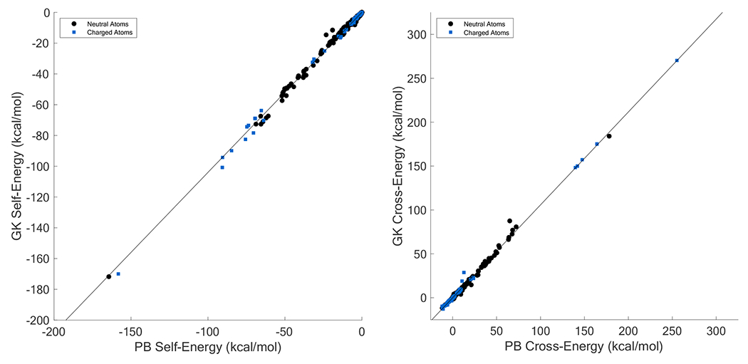
Panel A: Fit of GK self energies to perfect PB self energies (Y = 1.040X + 0.048, R² = 0.996). Panel B: Fit of GK cross term energies to perfect PB cross tenn energies (Y = 1.059X − 0.089, R² = 0.994). Both self and aggregate cross-term energies are reported for 1424 atoms.

Target Function for Electrostatic Radii Optimization

Electrostatic radii for 41 atom types were fit using the following target function

$$\text{E}\left(\mathbf{P}\right)={\text{W}}_{\text{MUE}}\sum _{i=1}^n{\left({\Delta \text{G}}_{\text{i}}^{\text{Expt}}-{\Delta \text{G}}_i^{\text{Model}}\left(\mathbf{P}\right)\right)}^2+{\text{W}}_{\text{MSE}}{\left(\sum _{i=1}^n{\Delta \text{G}}_i^{\text{Expt}}-\sum _{i=1}^n{\Delta \text{G}}_i^{\text{Model}}\left(\mathbf{P}\right)\right)}^2+{\text{W}}_{\text{Regularization}}\sum _{i=1}^{N_{\text{radii}}}{\left(R_i^{\text{Model}}-R_i^{\text{vdW}}\right)}^2$$ Equation 36.

where the first term favors minimizing the unsigned error between experimental and model solvation free energy over n molecules, the second term favors minimizing the overall signed error, and the final term penalizes electrostatic radii that deviate from the AMOEBA force field definition of minimum energy van der Waals separation (R_min). The optimization was performed using an L-BFGS minimizer for each of the APBS, ddCOSMO, and GK models. The optimization was seeded with electrostatic radii based on AMOEBA van der Waals R_min values, and after trial and error all three optimization weights were set to 1.0.

Results

Small Molecule Hydration Free Energy

The nonpolar portion of the model consists of an unfavorable cavitation free energy term and a favorable dispersion free energy term. One tunable parameter – solvent pressure – was used in calculating cavitation and two tunable parameters – a dispersion offset and an atomic overlap scale factor – were used in calculating dispersion. The solvent pressure of 0.0334 kcal/mol/ų for cavitation was chosen based on previous testing. The dispersion integral offset (d = 1.056 Å) and unitless HCT dispersion atomic overlap scale factor (s = 0.75) were chosen to match dispersion values from solute-solvent enthalpy simulations in explicit water (Supplementary Table S1).

For the electrostatic portion of the model, a total of 41 solute radii classes were optimized using L-BFGS minimization as described above. Solvation free energy difference values from the FreeSolv database^{71, 72} were used as experimental targets. Each radii class was determined based on SMARTS strings that were automatically generated for each atom type by PolType2. A total of 78 unique SMARTS strings were generated for the test set of 103 molecules. These 78 SMARTS strings were then reduced into 41 groups based on element, chemical environment, and electrostatic radii sizes from an initial optimization using all SMARTS strings under GK electrostatics (Supplementary Table S2). The use of fewer parameters helps to avoid overfitting and improve generalizability. Optimization was performed using the 41 radii classes to parameterize the APBS, ddCOSMO, and GK electrostatic models¹²¹. Parameterized radii deviated from original AMOEBA van der Waals radii by an average of 9.3% for APBS, 9.9% for ddCOSMO, and 14.9% for GK. The quality of the resulting implicit solvent model for small molecules using APBS, ddCOSMO, and GK is shown below in Figures 8, 9, and 10, respectively, and full data is available in Supplementary Tables S3–S8.

Figure 8.

Shown is a comparison of experimental and APBS solvation free energy differences using either AMOEBA van der Waals R_min radii to describe the solute-solvent boundary (Panel A) or using fit radii (Panel B). When using AMOEBA R_min radii, the linear regression gave Y = 0.9683 · X + 0.3215 with R² = 0.9702. When using fit radii, the linear regression gave Y = 1.0080 · X + 0.1416 with R² = 0.9979.

Figure 9.

Shown is a comparison of experimental and ddCOSMO solvation free energy differences using either AMOEBA van der Waals R_min radii to describe the solute-solvent boundary (Panel A) or using fit radii (Panel B). When using AMOEBA R_min radii, the linear regression gave Y = 1.0017 · X − 0.1465 with R² = 0.9738. When using fit radii, the linear regression gave Y = 1.0001 · X + 0.0015 with R² = 0.9981.

The data shown in Figures 8–10 is summarized Tables 1A and 1B, which give the root mean square error (RMSE) and mean signed error (MSE) between experimental and computed solvation free energy differences. Overall, parameterized solute radii resulted in RMSE/MUE MSE values of 1.00/0.70/0.05, 0.92/0.63/0.00, and 0.75/0.58/0.00 kcal/mol for the APBS, ddCOSMO, and GK models, respectively (Table 1B).

Figure 10.

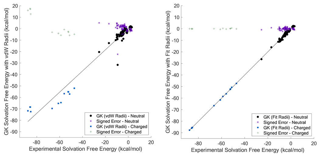
Shown is a comparison of experimental and GK solvation free energy differences using either AMOEBA van der Waals R_min radii to describe the solute-solvent boundary (Panel A) or using fit radii (Panel B). When using AMOEBA R_min radii, the linear regression gave Y = 0.9245 · X + 0.0360 with R² = 0.9567. When using fit radii, the linear regression gave Y = 0.9999 · X − 0.0046 with R² = 0.9987.

Table 1A.

RMSE/MSE for test molecules using AMOEBA van der Waals radii are given by functional group categories and overall (kcal/mol).

		AMOEBA Radii
Functional Group	N	APBS	ddCOSMO	GK
Alkanes	18	0.50/−0.24	0.71/−0.47	1.16/−0.89
Alcohols and Phenols	16	1.48/+1.27	2.02/−0.19	2.40/+2.09
Amines	12	2.51/+2.40	2.36/+2.17	3.04/+1.10
Amides	8	2.25/+1.98	1.28/+0.40	3.18/+2.63
Nitrogen Heterocyclic	8	2.02/+0.99	1.93/+0.14	2.33/+1.60
Arenes	5	0.77/−0.57	0.95/−0.56	1.35/−0.54
Ethers	5	0.86/+0.80	0.74/+0.49	1.45/+1.41
Oxanes and Oxines	4	1.05/+0.79	0.58/−0.16	2.29/+1.75
Thiols	4	1.68/−1.63	1.25/−1.16	1.93/−1.85
Carboxylic Acids	3	1.31/+1.18	0.68/+0.38	2.58/+2.39
Sulfides	3	1.20/−1.17	0.61/−0.48	1.49/−1.46
Aldehydes	2	0.61/+0.58	0.22/−0.16	1.52/+1.52
Other	3	1.55/+0.49	3.01/−1.38	13.04/−6.04
Total Neutrals	91	1.58/+0.76	1.58/+0.09	3.22/+0.62
Charged	12	9.90/+0.01	9.13/−2.12	9.80/+2.80
Total	103	3.69/+0.67	3.45/−0.17	4.51/+0.87

Table 1B.

RMSE/MSE for test molecules using parameterized electrostatic radii are given by functional group categories and overall (kcal/mol).

		Fit Solute Radii
Functional Group	N	APBS	ddCOSMO	GK
Alkanes	18	0.49/−0.24	0.42/−0.20	0.49/−0.17
Alcohols and Phenols	16	1.01/+0.50	1.31/+0.65	1.00/+0.56
Amines	12	1.49/+0.92	1.37/+0.06	0.92/−0.20
Amides	8	0.66/+0.13	0.66/+0.13	0.76/−0.12
Nitrogen Heterocyclic	8	1.31/+0.56	0.50/+0.07	0.88/+0.27
Arenes	5	0.50/−0.44	1.00/−0.61	0.80/−0.20
Ethers	5	0.23/−0.03	0.35/−0.11	0.57/−0.36
Oxanes and Oxines	4	1.16/−0.33	0.58/−0.36	1.05/+0.07
Thiols	4	0.65/−0.49	0.38/−0.26	0.32/−0.09
Carboxylic Acids	3	0.09/−0.08	0.11/−0.01	0.24/+0.00
Sulfides	3	0.36/−0.33	0.19/+0.09	0.32/−0.29
Aldehydes	2	0.48/−0.38	0.39/−0.39	0.11/−0.03
Other	3	1.96/−0.06	0.88/−0.56	0.51/−0.31
Total Neutrals	91	0.97/+0.14	0.87/+0.01	0.76/+0.00
Charged	12	1.18/−0.59	1.25/−0.07	0.73/−0.03
Total	103	1.00/+0.05	0.92/+0.00	0.75/+0.00

Comparison to Explicit Solvent Free Energy Differences

Although the implicit solvents described here were fit to experimental data, direct comparison to AMOEBA explicit solvent hydration free energy differences helps illuminate if the continuum models are either overfit or exhibit relatively higher errors. A subset of 26 neutral small molecules used to parameterize the implicit solvent model are compared to available data from a recent AMOEBA explicit solvent study¹²² in Table 2. Explicit solvent gave an RMSE of 0.70 kcal/mol compared to experiment, while implicit solvents using APBS, ddCOSMO, and GK electrostatics gave RMSEs of 0.91, 0.65, and 0.63 kcal/mol, respectively. The concordance between the RMSEs for the explicit and implicit hydration free energy differences support the conclusion that the continuum models are neither clearly overfit nor of worse quality than what is observed for AMOEBA solutes in explicit solvent.

Table 2.

Comparison of solvation free energy differences in AMOEBA explicit and implicit solvents to experimental solvation free energy differences (all values in kcal/mol).

		Explicit Solvent		ΔGimplicit			Signed Error
Molecule	ΔGexpt	ΔG	Error	APRS	COSMO	GK	APRS	COSMO	GK
isopropanol	−4.74	−4.21	0.28	−3.77	−3.66	−3.92	0.97	1.08	0.82
hydrogen sulfide	−0.70	−0.41	0.08	−1.06	−0.77	−0.80	−0.36	−0.07	−0.10
p-cresol	−6.13	−5.6	0.28	−6.22	−5.37	−4.99	−0.09	0.76	1.14
dimethylsulfide	−1.61	−1.85	0.06	−2.11	−1.56	−1.99	−0.50	0.05	−0.38
phenol	−6.60	−5.05	2.40	−6.23	−5.48	−5.49	0.37	1.12	1.11
benzene	−0.90	−1.23	0.11	−1.30	−1.70	−1.54	−0.40	−0.80	−0.64
ethanol	−5.00	−4.69	0.10	−4.09	−3.89	−3.57	0.91	1.11	1.43
ethane	1.83	1.73	0.01	2.31	2.10	2.54	0.48	0.27	0.71
n-butane	2.10	1.11	0.98	2.09	2.21	1.80	−0.01	0.11	−0.30
methylamine	−4.55	−5.46	0.83	−4.00	−4.53	−4.71	0.55	0.02	−0.16
dimethylamine	−4.29	−3.04	1.56	−2.72	−4.03	−5.48	1.57	0.26	−1.19
trimethylamine	−3.20	−2.09	1.23	−3.34	−3.09	−1.78	−0.14	0.11	1.42
propane	2.00	1.69	0.10	2.24	2.28	2.39	0.24	0.28	0.39
methane	2.00	1.73	0.07	2.43	2.39	1.89	0.43	0.39	−0.11
methanol	−5.10	−4.79	0.10	−3.55	−3.51	−3.40	1.55	1.59	1.70
n-propanol	−4.85	−4.85	0.00	−4.33	−4.53	−4.23	0.52	0.32	0.62
toluene	−0.90	−1.53	0.40	−1.41	−1.60	−1.12	−0.51	−0.70	−0.22
ethylbenzene	−0.79	−0.8	0.00	−1.21	−1.41	−0.87	−0.42	−0.62	−0.08
n-methylacetamide	−10.00	−8.66	1.80	−9.50	−9.09	−9.05	0.50	0.91	0.95
water	−6.30	−5.86	0.19	−5.36	−6.34	−6.27	0.94	−0.04	0.03
acetic acid	−6.69	−5.63	1.12	−6.56	−6.75	−6.37	0.13	−0.06	0.32
methylethylsulfide	−1.50	−1.98	0.23	−1.64	−1.19	−1.89	−0.14	0.31	−0.39
imidazole	−9.63	−10.25	0.38	−9.43	−9.79	−9.36	0.20	−0.16	0.27
acetamide	−9.70	−9.3	0.16	−10.78	−10.22	−10.46	−1.08	−0.52	−0.76
ethylamine	−4.50	−4.33	0.03	−4.14	−4.97	−4.28	0.36	−0.47	0.22
pyrrolidine	−5.48	−4.88	0.36	−2.31	−4.61	−4.24	3.17	0.87	1.24
MSE			0.19				0.36	0.24	0.31
MUE			0.57				0.64	0.50	0.64
RMSE			0.70				0.91	0.65	0.63

Validation Simulations on Proteins, DNA and RNA

Nine nucleic acids (≤ 24 nucleotides) and nine proteins (≤ 129 residues) of modest size were used to test the electrostatic energy and polarization response of the implicit solvents. Of the nucleic acids, seven were RNA and two were DNA. Starting structures for all 18 validation set molecules are shown in Figure 11 and were obtained from the Protein Data Bank (PDB). In the case of NMR ensembles, the first conformer was used. For explicit solvent simulations, each molecule was solvated in an explicit water box with neutralizing sodium or chloride ions. With the validation set molecule fixed, minimization to an RMS gradient of 0.1 kcal/mol/Å was performed on each system to allow relaxation of the water and ions.

Figure 11.

The validation set includes nine nucleic acids and nine proteins. The nucleic acid set can be further broken down into sets of four RNA helices (2JXQ, 1F5G, 1MIS, and 2L8F), three RNA hair pins (1ZIH, 2KOC, and 1SZY), and two DNA double helices (1D20 and 2HKB). Additional information on individual molecules and simulation conditions can be found in Supplementary Table S10. Coordinate files for each molecule (Tinker “XYZ” format) are provided in the Supporting Information.

Electrostatic energies were calculated for each validation set molecule with van der Waals and fit radii using all three electrostatics models. When using van der Waals radii (Figure 12A), the mean GK electrostatic energy was 1.65% more positive than APBS (R² = 0.9999), while that for ddCOSMO was 6.71% more negative (R² = 0.9990). The relatively large disparity between ddCOSMO and APBS when using identical van der Waals radii suggests that the COSMO approximation is not entirely ameliorated by its empirical scaling function. When using fit radii (Figure 12A), the mean GK electrostatic energy was 0.01% more negative than APBS (R² = 0.9991), while that for ddCOSMO was 0.11% more positive (R² = 0.9991). This shows that the COSMO approximation is compensated for to a large degree implicitly during the fitting of electrostatic radii. The slight reduction in R² between APBS and GK electrostatic energies moving from van der Waals radii to fit radii suggests that use a of single HCT overlap scale factor is not perfectly transferable across the range of atomic sizes found in proteins and nucleic acids. The optimization of element-specific HCT scale factors for GK electrostatics will be explored in future work that also focuses on handling interstitial spaces too small to accommodate water molecules (i.e. calculation of Born radii based on integration over a molecular volume rather than a van der Waals volume).

Figure 12.

The APBS energy values for the biomolecular validation set are plotted vs. ddCOSMO and GK for both van der Waals radii and fit radii. Panel A. APBS electrostatics energy using van der Waals radii vs ddCOSMO (Y = 1.0523X, R² = 0.9990) and GK (Y = 0.9854X, R² = 0.9999). Panel B. APBS PBE electrostatics energy using fit radii vs ddCOSMO (Y = 0.9884X, R² = 0.9991) and GK (Y = 0.9833X, R² = 0.9991). Full data is available in Supplementary Tables S11 and S13.

Dipole moment magnitudes were calculated for each validation set molecule in vacuum, explicit solvent, and implicit solvent. Prior to computing explicit solvent dipole moments, a series of short molecular dynamics (MD) simulations were used to equilibrate the system. Ensemble average dipole moment values were then calculated from 1 nsec MD simulations with the biomolecule fixed (i.e. solvent degrees of freedom were converged). For detailed simulation conditions, see Supplementary Table S10. In addition, dipole moment magnitudes were calculated for the validation set using three fixed charge force fields – AMBER ff99SB¹²³, OPLS-AA/L¹²⁴, and CHARMM22/CMAP¹²⁵, ¹²⁶. Tinker version 8.8.1 (August 2020) did not include nucleic acid force field parameters for OPLS-AA/L or CHARMM22/CMAP, so only AMOEBA and AMBER ff99SB dipole moment magnitudes are reported for nucleic acids. Dipole moment magnitudes calculated using available force fields for nucleic acids and proteins are presented in Figure 13. All fixed charge dipole moment magnitudes are plotted against ensemble average AMOEBA explicit solvent dipole moment magnitudes, as well as AMOEBA vacuum dipole moments. AMBER ff99SB, OPLS-AA/L, and CHARMM22/CMAP dipole moment magnitudes had R-squared values of 0.987, 0.979, and 0.982, respectively, when compared to AMOEBA vacuum dipole moment magnitudes, and R-squared values of 0.998, 0.996, and 0.996, respectively, when compared to AMOEBA explicit solvent dipole moment magnitudes. The better agreement of the fixed charge force fields with AMOEBA in explicit (or implicit) solvent, relative to worse agreement with AMOEBA in vacuum, is consistent with fixed charge biomolecular force fields being pre-polarized for aqueous simulations. This also demonstrates that the AMOEBA electrostatics model produces molecular dipole moments that are consistent with previous generation force fields.

Figure 13.

Comparison of dipole moment magnitudes for fixed charge force fields and AMOEBA across environments. Panel A: AMOEBA vacuum dipole moment magnitudes vs those for fixed charge force fields (AMBER ff99SB R²: 0.987, OPLS-AA/L R²: 0.979, CHARMM22/CMAP R²: 0.982). Panel B: AMOEBA explicit solvent dipole moment magnitudes vs those for fixed charge force fields (AMBER ff99SB R²: 0.998, OPLS-AA/L R²: 0.996, CHARMM22/CMAP R²: 0.996). Dotted lines at x = y are to guide the eye.

AMOEBA implicit solvent dipole moment magnitudes were calculated using each of the three parameterized electrostatics models and compared to those from explicit solvent ensemble averages as shown in Figure 14. All three electrostatics models achieved near perfect correlation with explicit solvent values based on R-squared values for the APBS, ddCOSMO, and GK models of 0.999 in each case. Notably, each AMOEBA implicit solvent electrostatic model produces dipoles moments that agree more closely with AMOEBA in explicit solvent than does any fixed charge force field. This supports the conclusion that if the AMOEBA biomolecular dipole moments are closer to reality than those from any of the fixed charge model, then AMOEBA simulations in implicit solvent are in some ways more realistic than fixed charge simulations in explicit solvent. The relative merits of fixed charge explicit water simulations compared to polarizable implicit solvent simulations will be explored more in the future. For Figure 14, dipole moment magnitudes for the APBS electrostatics model were calculated without implicitly adding ions. A full comparison of dipole moment magnitudes and electrostatic energy components for all validation set molecules is available in Supplementary Tables S11–S13. This includes dipole moment magnitudes calculated in APBS using the non-linear and linearized forms of the PBE with 150 mM salt. Overall, these results suggest the electrostatics models scale up well from initial optimization against small molecule hydration free energy differences to applications on larger biomolecules.

Figure 14.

Comparison of dipole moment magnitudes for AMOEBA in explicit solvent vs. vacuum, PB, ddCOSMO and GK environments for the validation set (vacuum R²: 0.990, PB/ddCOSMO/GK R²: 0.999 in each case). The dotted line at x = y is to guide the eye.

The performance of the APBS, ddCOSMO, and GK electrostatics models implemented in Tinker were compared by timing an energy and gradient calculation on a single CPU core (Intel® Xeon® CPU E5-2680 v4 at 2.40 GHz). Calculations were performed for one nucleic acid (1ZIH) and one protein (1VII) from the validation set. Results in Table 3 show that APBS is the costliest model, while GK is currently the most efficient. Timings for the same systems using AMOEBA/GK electrostatics implemented within FFX-OpenMM and executing on single GPU (NVIDIA® GeForce® RTX 2080 Ti) were also collected. The latter performance (less than 0.005 seconds per time step) is consistent with molecular dynamics performance of ~20 nsec per day using a conservative 1 fsec integration scheme, which opens the door to tuning the AMOEBA/GK continuum model using extensive simulations of proteins and nucleic acids. As of this writing, the APBS and ddCOSMO electrostatics models are not yet available for use on GPUs.

Table 3.

Performance of the APBS, ddCOSMO, and GK electrostatics models implemented in Tinker on a single CPU core; and for the GK model using FFX-OpenMM on a single GPU.

	Calculation of the Energy and Gradient (seconds)
	Tinker (1 CPU Thread)			FFX-OpenMM (1 GPU)
Molecule	APBS	ddCOSMO	GK	GK
1ZIH	48.804	11.285	0.250	0.0042
1VII	53.772	21.245	0.533	0.0047

Conclusions

Implicit solvent models were developed for use with the polarizable AMOEBA force field. Novel cavitation and dispersion non-polar terms were designed to replicate explicit solvent free energy differences using only three free parameters – a single cavitation parameter to describe solvent pressure for small cavities and two dispersion parameters (one to define the beginning of the dispersal integral and a second to account for atomic overlaps during integration). Based on these non-polar terms, the solute-solvent electrostatic boundary (i.e. atomic radii) was optimized for three continuum electrostatics models – ABPS, ddCOSMO, and GK – using numerical optimization against experimental small molecule solvation free energy differences. Overall, the APBS, ddCOSMO, and GK models produced mean unsigned errors of 0.70, 0.63, and 0.58 kcal/mol compared to experiment. All three implicit solvent models produced hydration free energy difference RMSEs within 0.2 kcal/mol of AMOEBA explicit solvent solvation free energy difference simulations for a collection of 26 small molecules (Table 2). This supports the conclusion that the implicit solvent models presented here are of similar quality to explicit solvent for hydration free energy differences and are not clearly overfit to the test data (i.e. overfitting might be suggested by implicit solvent RMSEs that are artificially much lower than those achieved by explicit solvent simulations).

Each small molecule used to parameterize the implicit solvent model fell within the volume scaling regime of the cavitation model, such that the contribution to solvation was calculated using SEV. For larger proteins or nucleic acids, the cavitation free energy of the model will fall within the surface area scaling regime. A future goal is to account for local molecular curvature to promote transferability of cavitation free energy to biomolecules of complex shapes. The dispersion model integrates the WCA attractive potential for each atom in the solute. This analytic, pairwise approach is well equipped to handle non-spherical solutes, which adds physical detail to the previously described Born radii-based dispersion model⁷³. Both the cavitation and dispersion models described here are currently limited by their lack of treatment of interstitial spaces, which is elaborated on below.

To optimize agreement of GK self-energies with calculated perfect PB multipolar selfenergies, it may be beneficial to use separate HCT scaling factors for each chemical element, instead of a single parameter as was done here. Precedent for this split is given in the original description of the HCT pairwise descreening approximation, where the scale factor magnitude generally decreases with increasing atomic size³⁴. Additionally, agreement between GK cross term energies and calculated perfect PB multipolar cross term energies might be improved by using separate generalizing function constants for monopoles, dipoles, and quadrupoles, rather than a single constant. The physical motivation is that the electrostatic potential is of longer range for monopoles than for dipoles. Therefore, the transition between the Born ion regime (or Kirkwood multipole regime) and the Coulomb regime, which is tuned by the constant in the generalizing function (Equation 34), could in principle be optimized for each multipole order separately. For simplicity, this work used a single HCT scale factor (0.72) and a single generalizing constant (2.455) for GK.

At the length scale of small molecules, continuum electrostatics is known to be sensitive to the definition of the solute-solvent boundary^127–131, and thus optimization of electrostatic radii is required to implicitly account for physical details like solute-water hydrogen bonding. Overall, the quality of the resulting models using fit solute radii for PB (RMSE 1.0, MSE 0.1), ddCOSMO (RMSE 0.9, MSE 0.0), and GK (RMSE 0.8, MSE 0.0) is comparable to the recent Drude/PB implicit solvent (RMSE 0.8, MSE 0.0)⁵¹. The fit radii reproduce experimental solvation free energy differences better than original van der Waals radii, which gave RMS errors of 3.69, 3.45, and 4.51 kcal/mol for APBS, ddCOSMO, and GK, respectively (Table 1A). Additionally, it may be beneficial to consider using optimized GK (or ddCOSMO) electrostatic radii as a starting point for electrostatics calculations in quantum mechanical continuum solvents^{61, 132}.

Dipole moment calculations using each AMOEBA implicit solvent for 18 protein and nucleic acid biomolecules show nearly exact agreement with explicit solvent dipole moments computed by averaging over solvent degrees of freedom (Figure 14). This suggests that all three models (APBS, ddCOSMO, and GK) successfully reproduce the polarization response observed in explicit water simulations at the resolution of overall biomolecules. Future work will focus on molecular dynamics simulations of biomolecules in implicit solvent compared to explicit solvent to access stability and the agreement of conformational ensembles. Furthermore, although the implicit solvent models discussed here have been developed for use with the AMOEBA polarizable force field, their support for polarizable atomic multipole electrostatics should permit adaptation to emerging models such as AMOEBA+ and HIPPO^133–135.

An important limitation of the current models is their focus on the use of a van der Waals description of the solute for cavitation, dispersion, and electrostatic contributions, rather than a molecular surface^{136, 137} The approximation of a van der Waals description is modest for small solutes but becomes problematic as molecular size and complexity increases (e.g. for biomolecules). For example, a simple van der Waals surface does not account for interstitial spaces (i.e. spaces between biomolecular residues or domains where water molecules cannot fit), and thereby allows continuum water access to spaces not accessible to explicit water. Favorable hydration effects of continuum water in interstitial spaces promotes swelling of biomolecules and opposes hydrophobic compaction forces. For this reason, future work will incorporate methods that have been proposed to account for interstitial spaces^{119, 137–139} into the AMOEBA family of implicit solvents.

References

- 1.Chandler D, Interfaces and the driving force of hydrophobic assembly. Nature 2005, 437 (7059), 640–647. [DOI] [PubMed] [Google Scholar]
- 2.Dill KA; MacCallum JL, The Protein-Folding Problem, 50 Years On. Science 2012, 338 (6110), 1042–1046. [DOI] [PubMed] [Google Scholar]
- 3.Zhang QC; Petrey D; Deng L; Qiang L; Shi Y; Thu CA; Bisikirska B; Lefebvre C; Accili D; Hunter T; Maniatis T; Califano A; Honig B, Structure-based prediction of protein-protein interactions on a genome-wide scale. Nature 2012, 490 (7421), 556–60. [DOI] [PMC free article] [PubMed] [Google Scholar]
- 4.Ren P; Chun J; Thomas DG; Schnieders MJ; Marucho M; Zhang J; Baker NA, Biomolecular electrostatics and solvation: a computational perspective. Q. Rev. Biophys 2012, 45 (4), 427–91. [DOI] [PMC free article] [PubMed] [Google Scholar]
- 5.LuCore Stephen D.; Litman Jacob M.; Powers Kyle T.; Gao S; Lynn Ava M.; Tollefson William T. A.; Fenn Timothy D.; Washington MT; Schnieders Michael J., Dead-end elimination with a polarizable force field repacks PCNA structures. Biophys. J 2015, 109 (4), 816–826. [DOI] [PMC free article] [PubMed] [Google Scholar]
- 6.Huang P-S; Boyken SE; Baker D, The coming of age of de novo protein design. Nature 2016, 537, 320. [DOI] [PubMed] [Google Scholar]
- 7.Hallen MA; Martin JW; Ojewole A; Jou JD; Lowegard AU; Frenkel MS; Gainza P; Nisonoff HM; Mukund A; Wang S; Holt GT; Zhou D; Dowd E; Donald BR, OSPREY 3.0: Open-source protein redesign for you, with powerful new features. J. Comput. Chem 2018, 39 (30), 2494–2507. [DOI] [PMC free article] [PubMed] [Google Scholar]
- 8.Villa F; Panel N; Chen XY; Simonson T, Adaptive landscape flattening in amino acid sequence space for the computational design of protein:peptide binding. J. Chem. Phys 2018, 149 (7), 8. [DOI] [PubMed] [Google Scholar]
- 9.Tollefson MR; Litman JM; Qi G; O’Connell CE; Wipfler MJ; Marini RJ; Bernabe HV; Tollefson WTA; Braun TA; Casavant TL; Smith RJH; Schnieders MJ, Structural insights into hearing loss genetics from polarizable protein repacking. Biophys. J 2019, 117 (3), 602–612. [DOI] [PMC free article] [PubMed] [Google Scholar]
- 10.Cheatham TE; Case DA, Twenty-five years of nucleic acid simulations. Biopolymers 2013, 99 (12), 969–977. [DOI] [PMC free article] [PubMed] [Google Scholar]
- 11.Bergonzo C; Henriksen NM; Roe DR; Cheatham TE, Highly sampled tetranucleotide and tetraloop motifs enable evaluation of common RNA force fields. Rna 2015, 21 (9), 1578–1590. [DOI] [PMC free article] [PubMed] [Google Scholar]
- 12.Musil M; Konegger H; Hong J; Bednar D; Damborsky J, Computational Design of Stable and Soluble Biocatalysts. Acs Catalysis 2019, 9 (2), 1033–1054. [Google Scholar]
- 13.Roux B; Simonson T, Implicit solvent models. Biophys. Chem 1999, 78 (1–2), 1–20. [DOI] [PubMed] [Google Scholar]
- 14.Onufriev AV; Izadi S, Water models for biomolecular simulations. Wiley Interdiscip. Rev.-Comput. Mol. Sci 2018, 8 (2), 40. [Google Scholar]
- 15.Tan C; Tan YH; Luo R, Implicit nonpolar solvent models. J. Phys. Chem. B 2007, 111 (42), 12263–12274. [DOI] [PubMed] [Google Scholar]
- 16.Decherchi S; Masetti M; Vyalov I; Rocchia W, Implicit solvent methods for free energy estimation. Eur. J. Med. Chem 2015, 91, 27–42. [DOI] [PMC free article] [PubMed] [Google Scholar]
- 17.Levy RM; Zhang LY; Gallicchio E; Felts AK, On the nonpolar hydration free energy of proteins: Surface area and continuum solvent models for the solute-solvent interaction energy. J. Am. Chem. Soc 2003, 125 (31), 9523–9530. [DOI] [PubMed] [Google Scholar]
- 18.Wagoner JA; Baker NA, Assessing implicit models for nonpolar mean solvation forces: the importance of dispersion and volume terms. Proc. Natl. Acad. Sci. U. S. A 2006, 103 (22), 8331–8336. [DOI] [PMC free article] [PubMed] [Google Scholar]
- 19.Chen Z; Zhao S; Chun J; Thomas DG; Baker NA; Bates PW; Wei GW, Variational approach for nonpolar solvation analysis. J. Chem. Phys 2012, 137 (8), 9. [DOI] [PMC free article] [PubMed] [Google Scholar]
- 20.Harris RC; Pettitt BM, Effects of geometry and chemistry on hydrophobic solvation. Proc. Natl. Acad. Sci. U. S. A 2014, 111 (41), 14681–14686. [DOI] [PMC free article] [PubMed] [Google Scholar]
- 21.Michael E; Polydorides S; Simonson T; Archontis G, Simple models for nonpolar solvation: parameterization and testing. J. Comput. Chem 2017, 38 (29), 2509–2519. [DOI] [PubMed] [Google Scholar]
- 22.Gilson MK; Honig BH, Calculation of electrostatic potentials in an enzyme active-site. Nature 1987, 330 (6143), 84–86. [DOI] [PubMed] [Google Scholar]
- 23.Gilson MK; Honig B, Calculation of the total electrostatic energy of a macromolecular system - solvation energies, binding-energies, and conformational-analysis. Proteins-Structure Function and Genetics 1988, 4 (1), 7–18. [DOI] [PubMed] [Google Scholar]
- 24.Jeancharles A; Nicholls A; Sharp K; Honig B; Tempczyk A; Hendrickson TF; Still WC, Electrostatic contributions to solvation energies - comparison of free-energy perturbation and continuum calculations. J. Am. Chem. Soc 1991, 113 (4), 1454–1455. [Google Scholar]
- 25.Honig B; Nicholls A, Classical electrostatics in biology and chemistry. Science 1995, 268 (5214), 1144–1149. [DOI] [PubMed] [Google Scholar]
- 26.Baker NA; Sept D; Joseph S; Holst MJ; McCammon JA, Electrostatics of nanosystems: application to microtubules and the ribosome. Proc. Natl. Acad. Sci. U.S.A 2001, 98 (18), 10037–41. [DOI] [PMC free article] [PubMed] [Google Scholar]
- 27.Simonson T, Macromolecular electrostatics: continuum models and their growing pains. Curr. Opin. Struct. Biol 2001, 11 (2), 243–252. [DOI] [PubMed] [Google Scholar]
- 28.Kollman PA; Massova I; Reyes C; Kuhn B; Huo SH; Chong L; Lee M; Lee T; Duan Y; Wang W; Donini O; Cieplak P; Srinivasan J; Case DA; Cheatham TE, Calculating structures and free energies of complex molecules: Combining molecular mechanics and continuum models. Acc. Chem. Res 2000, 33 (12), 889–897. [DOI] [PubMed] [Google Scholar]
- 29.Tan YH; Luo R, Continuum treatment of electronic polarization effect. J. Chem. Phys 2007, 126 (9), 6. [DOI] [PubMed] [Google Scholar]
- 30.Tan YH; Tan CH; Wang J; Luo R, Continuum polarizable force field within the Poisson-Boltzmann framework. J. Phys. Chem. B 2008, 112 (25), 7675–7688. [DOI] [PMC free article] [PubMed] [Google Scholar]
- 31.Jurrus E; Engel D; Star K; Monson K; Brandi J; Felberg LE; Brookes DH; Wilson L; Chen J; Liles K; Chun M; Li P; Gohara DW; Dolinsky T; Konecny R; Koes DR; Nielsen JE; Head-Gordon T; Geng W; Krasny R; Wei G-W; Holst MJ; McCammon JA; Baker NA, Improvements to the APBS biomolecular solvation software suite. Protein Sci. 2018, 27 (1), 112–128. [DOI] [PMC free article] [PubMed] [Google Scholar]
- 32.Rashin AA; Honig B, Reevaluation of the Born model of ion hydration. J. Phys. Chem 1985, 89 (26), 5588–5593. [Google Scholar]
- 33.Roux B; Yu HA; Karplus M, Molecular-basis for the Born model of ion solvation. J. Phys. Chem 1990, 94 (11), 4683–4688. [Google Scholar]
- 34.Hawkins GD; Cramer CJ; Truhlar DG, Pairwise solute descreening of solute charges from a dielectric medium. Chem. Phys. Lett 1995, 246 (1–2), 122–129. [Google Scholar]
- 35.Qiu D; Shenkin PS; Hollinger FP; Still WC, The GB/SA continuum model for solvation: a fast analytical method for the calculation of approximate Born radii. J. Phys. Chem. A 1997, 101 (16), 3005–14. [Google Scholar]
- 36.Nina M; Beglov D; Roux B, Atomic radii for continuum electrostatics calculations based on molecular dynamics free energy simulations. J. Phys. Chem. B 1997, 101 (26), 5239–5248. [Google Scholar]
- 37.Gallicchio E; Levy RM, AGBNP: An analytic implicit solvent model suitable for molecular dynamics simulations and high-resolution modeling. J. Comput. Chem 2004, 25 (4), 479–499. [DOI] [PubMed] [Google Scholar]
- 38.Gallicchio E; Paris K; Levy RM, The AGBNP2 implicit solvation model. J. Chem. Theory Comput 2009, 5 (9), 2544–2564. [DOI] [PMC free article] [PubMed] [Google Scholar]
- 39.Mukhopadhyay A; Aguilar BH; Tolokh IS; Onufriev AV, Introducing charge hydration asymmetry into the generalized Born model. J. Chem. Theory Comput 2014, 10 (4), 1788–1794. [DOI] [PMC free article] [PubMed] [Google Scholar]
- 40.Onufriev AV; Case DA, Generalized Born implicit solvent models for biomolecules. In Annual Review of Biophysics, Vol 48, Dill KA, Ed. Annual Reviews: Palo Alto, 2019; Vol. 48, pp 275–296. [DOI] [PMC free article] [PubMed] [Google Scholar]
- 41.Ren P; Wu C; Ponder JW, Polarizable atomic multipole-based molecular mechanics for organic molecules. J. Chem. Theory Comput 2011, 7 (10), 3143–3161. [DOI] [PMC free article] [PubMed] [Google Scholar]
- 42.Zhang C; Lu C; Jing Z; Wu C; Piquemal J-P; Ponder JW; Ren P, AMOEBA polarizable atomic multipole force field for nucleic acids. J. Chem. Theory Comput 2018, 14 (4), 2084–2108. [DOI] [PMC free article] [PubMed] [Google Scholar]
- 43.Schnieders MJ; Baker NA; Ren PY; Ponder JW, Polarizable atomic multipole solutes in a Poisson-Boltzmann continuum. J. Chem. Phys 2007, 126 (12), 124114. [DOI] [PMC free article] [PubMed] [Google Scholar]
- 44.Lipparini F; Lagardère L; Raynaud C; Stamm B; Cancès E; Mennucci B; Schnieders M; Ren P; Maday Y; Piquemal J-P, Polarizable Molecular Dynamics in a Polarizable Continuum Solvent. J. Chem. Theory Comput 2015, 11 (2), 623–634. [DOI] [PMC free article] [PubMed] [Google Scholar]
- 45.Schnieders MJ; Ponder JW, Polarizable atomic multipole solutes in a generalized Kirkwood continuum. J. Chem. Theory Comput 2007, 3 (6), 2083–2097. [DOI] [PMC free article] [PubMed] [Google Scholar]
- 46.Kirkwood JG, Theory of solutions of molecules containing widely separated charges with special application to zwitterions. J. Chem. Phys 1934, 2 (7), 351–361. [Google Scholar]
- 47.Maple JR; Cao YX; Damm WG; Halgren TA; Kaminski GA; Zhang LY; Friesner RA, A polarizable force field and continuum solvation methodology for modeling of protein-ligand interactions. J. Chem. Theory Comput 2005, 1 (4), 694–715. [DOI] [PubMed] [Google Scholar]
- 48.Cortis CM; Friesner RA, Numerical solution of the Poisson-Boltzmann equation using tetrahedral finite-element meshes. J. Comput. Chem 1997, 18 (13), 1591–1608. [Google Scholar]
- 49.Lemkul JA; Huang J; Roux B; MacKerell AD, An Empirical Polarizable Force Field Based on the Classical Drude Oscillator Model: Development History and Recent Applications. Chem. Rev 2016, 116 (9), 4983–5013. [DOI] [PMC free article] [PubMed] [Google Scholar]
- 50.Lemkul JA; MacKerell AD Jr., Polarizable force field for RNA based on the classical drude oscillator. J. Comput. Chem 2018, 39 (32), 2624–2646. [DOI] [PMC free article] [PubMed] [Google Scholar]
- 51.Aleksandrov A; Lin FY; Roux B; MacKerell AD, Combining the polarizable Drude force field with a continuum electrostatic Poisson-Boltzmann implicit solvation model. J. Comput. Chem 2018, 39 (22), 1707–1719. [DOI] [PMC free article] [PubMed] [Google Scholar]
- 52.Aleksandrov A; Roux B; MacKerell AD, pKa Calculations with the Polarizable Drude Force Field and Poisson–Boltzmann Solvation Model. J. Chem. Theory Comput 2020, 16 (7), 4655–4668. [DOI] [PMC free article] [PubMed] [Google Scholar]
- 53.MacKerell AD; Bashford D; Bellott M; Dunbrack RL; Evanseck JD; Field MJ; Fischer S; Gao J; Guo H; Ha S; Joseph-McCarthy D; Kuchnir L; Kuczera K; Lau FTK; Mattos C; Michnick S; Ngo T; Nguyen DT; Prodhom B; Reiher WE; Roux B; Schlenkrich M; Smith JC; Stote R; Straub J; Watanabe M; Wiorkiewicz-Kuczera J; Yin D; Karplus M, All-atom empirical potential for molecular modeling and dynamics studies of proteins. J. Phys. Chem. B 1998, 102 (18), 3586–616. [DOI] [PubMed] [Google Scholar]
- 54.Best RB; Zhu X; Shim J; Lopes PEM; Mittal J; Feig M; MacKerell AD, Optimization of the additive CHARMM all-atom protein force field targeting improved sampling of the backbone phi, psi and side-chain chi(1) and chi(2) dihedral angles. J. Chem. Theory Comput 2012, 8 (9), 3257–3273. [DOI] [PMC free article] [PubMed] [Google Scholar]
- 55.Poier PP; Jensen F, Including implicit solvation in the bond capacity polarization model. J. Chem. Phys 2019, 151 (11), 6. [DOI] [PubMed] [Google Scholar]
- 56.Poier PP; Jensen F, Polarizable charges in a generalized Born reaction potential. The Journal of Chemical Physics 2020, 153 (2), 024111. [DOI] [PubMed] [Google Scholar]
- 57.Cooper CD, A boundary-integral approach for the poisson-boltzmann equation with polarizable force fields. J. Comput. Chem 2019, 40 (18), 1680–1692. [DOI] [PubMed] [Google Scholar]
- 58.Cooper CD; Bardhan JP; Barba LA, A biomolecular electrostatics solver using Python, GPUs and boundary elements that can handle solvent-filled cavities and Stern layers. Computer Physics Communications 2014, 185 (3), 720–729. [DOI] [PMC free article] [PubMed] [Google Scholar]
- 59.Cramer CJ; Truhlar DG, Implicit solvation models: Equilibria, structure, spectra, and dynamics. Chem. Rev 1999, 99 (8), 2161–2200. [DOI] [PubMed] [Google Scholar]
- 60.Tomasi J, Thirty years of continuum solvation chemistry: a review, and prospects for the near future. Theor. Chem. Acc 2004, 112 (4), 184–203. [Google Scholar]
- 61.Tomasi J; Mennucci B; Cammi R, Quantum mechanical continuum solvation models. Chem. Rev 2005, 105 (8), 2999–3093. [DOI] [PubMed] [Google Scholar]
- 62.Mierts S; Scrocco E; Tomasi J, Electrostatic interaction of a solute with a continuum. A direct utilizaion of ab initio molecular potentials for the prevision of solvent effects. Chem. Phys 1981, 55(1), 117–129. [Google Scholar]
- 63.Cances E; Mennucci B; Tomasi J, A new integral equation formalism for the polarizable continuum model: Theoretical background and applications to isotropic and anisotropic dielectrics. J. Chem. Phys 1997, 107 (8), 3032–3041. [Google Scholar]
- 64.Cramer CJ; Truhlar DG, An SCF solvation model for the hydrophobic effect and absolute free energies of aqueous solvation. Science 1992, 256 (5054), 213–217. [DOI] [PubMed] [Google Scholar]
- 65.Kelly CP; Cramer CJ; Truhlar DG, SM6: A density functional theory continuum solvation model for calculating aqueous solvation free energies of neutrals, ions, and solute-water clusters. J. Chem. Theory Comput 2005, 1 (6), 1133–1152. [DOI] [PubMed] [Google Scholar]
- 66.Marenich AV; Cramer CJ; Truhlar DG, Universal solvation model based on solute electron density and on a continuum model of the solvent defined by the bulk dielectric constant and atomic surface tensions. J. Phys. Chem. B 2009, 113 (18), 6378–6396. [DOI] [PubMed] [Google Scholar]
- 67.Klamt A; Schuurmann G, COSMO - a new approach to dielectric screening in solvents with explicit expressions for the screening energy and its gradient. Journal of the Chemical Society: Perkin Transactions 2 1993, (5), 799–805. [Google Scholar]
- 68.Klamt A, Conductor-like screening model for real solvents - a new approach to the quantitative calculation of solvation phenomena. J. Phys. Chem 1995, 99 (7), 2224–2235. [Google Scholar]
- 69.Rackers JA; Wang Z; Lu C; Laury ML; Lagardère L; Schnieders MJ; Piquemal J-P; Ren P; Ponder JW, Tinker 8: Software Tools for Molecular Design. J. Chem. Theory Comput 2018, 14 (10), 5273–5289. [DOI] [PMC free article] [PubMed] [Google Scholar]
- 70.Stone AJ, Distributed multipole analysis: Stability for large basis sets. J. Chem. Theory Comput 2005, 1 (6), 1128–1132. [DOI] [PubMed] [Google Scholar]
- 71.Mobley DL; Guthrie JP, FreeSolv: a database of experimental and calculated hydration free energies, with input files. J. Comput.-Aided Mol. Des 2014, 28 (7), 711–720. [DOI] [PMC free article] [PubMed] [Google Scholar]
- 72.Matos GDR; Kyu DY; Loeffler HH; Chodera JD; Shirts MR; Mobley DL, Approaches for calculating solvation free energies and enthalpies demonstrated with an update of the FreeSolv database. J. Chem. Eng. Data 2017, 62 (5), 1559–1569. [DOI] [PMC free article] [PubMed] [Google Scholar]
- 73.Gallicchio E; Zhang LY; Levy RM, The SGB/NP hydration free energy model based on the surface Generalized Born solvent reaction field and novel nonpolar hydration free energy estimators. J. Comput. Chem 2002, 23 (5), 517–529. [DOI] [PubMed] [Google Scholar]
- 74.Rizzo RC; Aynechi T; Case DA; Kuntz ID, Estimation of absolute free energies of hydration using continuum methods: accuracy of partial charge models and optimization of nonpolar contributions. J. Chem. Theory Comput 2006, 2 (1), 128–139. [DOI] [PubMed] [Google Scholar]
- 75.Bartmess JE, “Negative ion energetics data”. In NIST Chemistry WebBook, Technology, N. I. o. S. a., Ed. Gaithersburg, MD, p 20899. [Google Scholar]
- 76.Hunter EP; Lias SG, “Proton affinity evaluation”. In NIST Chemistry WebBook, National Institute of Standards and Technology: Gaithersburg, MD, p 20899. [Google Scholar]
- 77.Stewart R, The proton: applications to organic chemistry. Academic Press, Inc.: New York, 1985; Vol. 46. [Google Scholar]
- 78.Wang Z Polarizable force field development, and applications to conformational sampling and free energy calculation. Dissertation, Washington University in St Louis, St Louis, MO, 2018. [Google Scholar]
- 79.Fawcett WR, Thermodynamic parameters for the solvation of monatomic ions in water. The Journal of Physical Chemistry B 1999, 103 (50), 11181–11185. [Google Scholar]
- 80.Ashbaugh HS, Convergence of molecular and macroscopic continuum descriptions of ion hydration. The Journal of Physical Chemistry B 2000, 104 (31), 7235–7238. [Google Scholar]
- 81.Wu JC; Chattree G; Ren PY, Automation of AMOEBA polarizable force field parameterization for small molecules. Theor. Chem. Acc 2012, 131 (3), 11. [DOI] [PMC free article] [PubMed] [Google Scholar]
- 82.Wu JC; Chattree G; Ren P, Automation of AMOEBA polarizable force field parameterization for small molecules. Theor. Chem. Acc 2012, 131 (3), 1–11. [DOI] [PMC free article] [PubMed] [Google Scholar]
- 83.Huang DM; Chandler D, Temperature and length scale dependence of hydrophobic effects and their possible implications for protein folding. Proc. Natl. Acad. Sci. U. S. A 2000, 97 (15), 8324–8327. [DOI] [PMC free article] [PubMed] [Google Scholar]
- 84.Huang DM; Geissler PL; Chandler D, Scaling of hydrophobic solvation free energies. J. Phys. Chem. B 2001, 105 (28), 6704–6709. [Google Scholar]
- 85.Huang DM; Chandler D, The hydrophobic effect and the influence of solute-solvent attractions. J. Phys. Chem. B 2002, 106 (8), 2047–2053. [Google Scholar]
- 86.Chen JH; Brooks CL, Critical importance of length-scale dependence in implicit modeling of hydrophobic interactions. J. Am. Chem. Soc 2007, 129 (9), 2444-+. [DOI] [PMC free article] [PubMed] [Google Scholar]
- 87.Connolly ML, Analytical molecular surface calculation. J. Appl. Crystallogr 1983, 16 (5), 548–558. [Google Scholar]
- 88.Connolly ML, Computation of molecular volume. J. Am. Chem. Soc 1985, 107 (5), 1118–1124. [Google Scholar]
- 89.Connolly ML, The molecular-surface package. J. Mol. Graph 1993, 11 (2), 139–143. [DOI] [PubMed] [Google Scholar]
- 90.Schnieders MJ Force Field X, Version 1.0. https://ffx.biochem.uiowa.edu.
- 91.Richards FM, Areas, volumes, packing and protein structure. Annual review of biophysics and bioengineering 1977, 6 (1), 151–176. [DOI] [PubMed] [Google Scholar]
- 92.Schnieders MJ The Theory and Effect of Solvation on Biomolecules. Dissertation, Washington University in St. Louis, St. Louis, MO, 2007. [Google Scholar]
- 93.Ren P; Ponder JW, Polarizable atomic multipole water model for molecular mechanics simulation. J. Phys. Chem. B 2003, 107 (24), 5933–5947. [Google Scholar]
- 94.Richmond TJ, Solvent accessible surface area and excluded volume in proteins: Analytical equations for overlapping spheres and implications for the hydrophobic effect. J. Mol. Biol 1984, 178 (1), 63–89. [DOI] [PubMed] [Google Scholar]
- 95.Kundrot CE; Ponder JW; Richards FM, Algorithms for calculating excluded volume and its derivatives as a function of molecule-conformation and their use in energy minimization. J. Comput. Chem 1991, 12 (3), 402–409. [Google Scholar]
- 96.Wesson L; Eisenberg D, Atomic solvation parameters applied to molecular-dynamics of proteins in solution. Protein Sci. 1992, 1 (2), 227–235. [DOI] [PMC free article] [PubMed] [Google Scholar]
- 97.Steam, I. A. f. t. P. o. W. In IAPWS release on surface tension of heavy water substance, Physical Chemistry of Aqueous Systems: Proceedings of the 12th International Conference on the Properties of Water and Steam, Orlando, FL, Orlando, FL, 1994; pp a107–a138. [Google Scholar]
- 98.Halgren TA, The representation of van der Waals (vdW) interactions in molecular mechanics force fields: potential form, combination rules, and vdW parameters. J. Am. Chem. Soc 1992, 114 (20), 7827–7843. [Google Scholar]
- 99.Weeks JD; Chandler D; Andersen HC, Role of repulsive forces in determining the equilibrium structure of simple liquids. The Journal of Chemical Physics 1971, 54 (12), 5237–5247. [Google Scholar]
- 100.Chandler D; Weeks JD; Andersen HC, Van der Waals picture of liquids, solids, and phase transformations. Science 1983, 220 (4599), 787–794. [DOI] [PubMed] [Google Scholar]
- 101.Gallicchio E; Kubo MM; Levy RM, Enthalpy-entropy and cavity decomposition of alkane hydration free energies: Numerical results and implications for theories of hydrophobic solvation. J. Phys. Chem. B 2000, 104 (26), 6271–6285. [Google Scholar]
- 102.Hawkins GD; Cramer CJ; Truhlar DG, Parametrized models of aqueous free energies of solvation based on pairwise descreening of solute atomic charges from a dielectric medium. J. Phys. Chem 1996, 100 (51), 19824–19839. [Google Scholar]
- 103.Lipparini F; Lagardère L; Stamm B; Cancès E; Schnieders M; Ren P; Maday Y; Piquemal J-P, Scalable Evaluation of Polarization Energy and Associated Forces in Polarizable Molecular Dynamics: I. Toward Massively Parallel Direct Space Computations. J. Chem. Theory Comput 2014, 10 (4), 1638–1651. [DOI] [PMC free article] [PubMed] [Google Scholar]
- 104.Aviat F; Levitt A; Stamm B; Maday Y; Ren P; Ponder JW; Lagardère L; Piquemal J-P, Truncated Conjugate Gradient: An Optimal Strategy for the Analytical Evaluation of the Many-Body Polarization Energy and Forces in Molecular Simulations. J. Chem. Theory Comput 2017, 13 (1), 180–190. [DOI] [PMC free article] [PubMed] [Google Scholar]
- 105.Simmonett AC; IV FCP; Ponder JW; Brooks BR, An empirical extrapolation scheme for efficient treatment of induced dipoles. The Journal of Chemical Physics 2016, 145 (16), 164101. [DOI] [PMC free article] [PubMed] [Google Scholar]
- 106.Lipparini F; Lagardere L; Scalmani G; Stamm B; Cances E; Maday Y; Piquemal JP; Frisch MJ; Mennucci B, Quantum calculations in solution for large to very large molecules: a new linear scaling QM/continuum approach. J. Phys. Chem. Lett 2014, 5 (6), 953–958. [DOI] [PubMed] [Google Scholar]
- 107.Lipparini F; Scalmani G; Lagardere L; Stamm B; Cances E; Maday Y; Piquemal JP; Frisch MJ; Mennucci B, Quantum, classical, and hybrid QM/MM calculations in solution: general implementation of the ddCOSMO linear scaling strategy. J. Chem. Phys 2014, 141 (18), 13. [DOI] [PubMed] [Google Scholar]
- 108.Stamm B; Lagardere L; Scalmani G; Gatto P; Cances E; Piquemal JP; Maday Y; Mennucci B; Lipparini F, How to make continuum solvation incredibly fast in a few simple steps: a practical guide to the domain decomposition paradigm for the conductor-like screening model. Int. J. Quantum Chem 2019, 119 (1), 15. [Google Scholar]
- 109.Rackers JA; Wang Z; Lu C; Laury ML; Lagardere L; Schnieders MJ; Piquemal J-P; Ren P; Ponder JW, Tinker 8: software tools for molecular design. J. Chem. Theory Comput 2018. [DOI] [PMC free article] [PubMed] [Google Scholar]
- 110.Holst M; Saied F, Multigrid solution of the Poisson-Boltzmann equation. J. Comput. Chem 1993, 14 (1), 105–113. [Google Scholar]
- 111.Holst MJ; Saied F, Numerical solution of the nonlinear Poisson-Boltzmann equation: developing more robust and efficient methods. J. Comput. Chem 1995, 16 (3), 337–364. [Google Scholar]
- 112.Klamt A; Moya C; Palomar J, A comprehensive comparison of the IEFPCM and SS(V)PE continuum solvation methods with the COSMO approach. J. Chem. Theory Comput 2015, 11 (9), 4220–4225. [DOI] [PubMed] [Google Scholar]
- 113.Baldridge K; Klamt A, First principles implementation of solvent effects without outlying charge error. The Journal of Chemical Physics 1997, 106 (16), 6622–6633. [Google Scholar]
- 114.Cossi M; Rega N; Scalmani G; Barone V, Energies, structures, and electronic properties of molecules in solution with the C-PCM solvation model. J. Comput. Chem 2003, 24 (6), 669–681. [DOI] [PubMed] [Google Scholar]
- 115.Lagardere L; Jolly LH; Lipparini F; Aviat F; Stamm B; Jing ZFF; Harger M; Torabifard H; Cisneros GA; Schnieders MJ; Gresh N; Maday Y; Ren PYY; Ponder JW; Piquemal JP, Tinker-HP: a massively parallel molecular dynamics package for multiscale simulations of large complex systems with advanced point dipole polarizable force fields. Chem. Sci 2018, 9 (4), 956–972. [DOI] [PMC free article] [PubMed] [Google Scholar]
- 116.Bashford D; Case DA, Generalized Born models of macromolecular solvation effects. Annu. Rev. Phys. Chem 2000, 51, 129–152. [DOI] [PubMed] [Google Scholar]
- 117.Grycuk T, Deficiency of the Coulomb-field approximation in the Generalized Born model: An improved formula for Born radii evaluation. J. Chem. Phys 2003, 119 (9), 4817–4826. [Google Scholar]
- 118.Mongan J; Svrcek-Seiler WA; Onufriev A, Analysis of integral expressions for effective Born radii. J. Chem. Phys 2007, 127 (18), 10. [DOI] [PubMed] [Google Scholar]
- 119.Aguilar B; Shadrach R; Onufriev AV, Reducing the secondary structure bias in the generalized Born model via R6 effective radii. J. Chem. Theory Comput 2010, 6 (12), 3613–3630. [Google Scholar]
- 120.Onufriev A; Case DA; Bashford D, Effective Born radii in the Generalized Born approximation: The importance of being perfect. J. Comput. Chem 2002, 23 (14), 1297–1304. [DOI] [PubMed] [Google Scholar]
- 121.Schnieders MJ; Ponder JW, Implicit solvents for the AMOEBA force field based on Poisson-Boltzmann and Generalized Kirkwood electrostatics (in preparation). [Google Scholar]
- 122.Ponder J; Wu C; Ren P; Pande V; Chodera J; Schnieders M; Haque I; Mobley D; Lambrecht D; DiStasio R; Head-Gordon M; Clark G; Johnson M; Head-Gordon T, Current status of the AMOEBA polarizable force field. J. Phys. Chem. B 2010, 114 (8), 2549–2564. [DOI] [PMC free article] [PubMed] [Google Scholar]
- 123.Hornak V; Abel R; Okur A; Strockbine B; Roitberg A; Simmerling C, Comparison of multiple amber force fields and development of improved protein backbone parameters. Proteins 2006, 65 (3), 712–725. [DOI] [PMC free article] [PubMed] [Google Scholar]
- 124.Kaminski GA; Friesner RA; Tirado-Rives J; Jorgensen WL, Evaluation and reparametrization of the OPLS-AA force field for proteins via comparison with accurate quantum chemical calculations on peptides. J. Phys. Chem. B 2001, 105 (28), 6474–6487. [Google Scholar]
- 125.Foloppe N; MacKerell AD, Conformational properties of the deoxyribose and ribose moieties of nucleic acids: a quantum mechanical study. J. Phys. Chem. B 1998, 102 (34), 6669–6678. [Google Scholar]
- 126.Buck M; Bouguet-Bonnet S; Pastor RW; MacKerell AD, Importance of the CMAP correction to the CHARMM22 protein force field: dynamics of hen lysozyme. Biophys. J 2006, 90 (4), L36–L38. [DOI] [PMC free article] [PubMed] [Google Scholar]
- 127.Nina M; Im W; Roux B, Optimized atomic radii for protein continuum electrostatics solvation forces. Biophys. Chem 1999, 78 (1-2), 89–96. [DOI] [PubMed] [Google Scholar]
- 128.Swanson JMJ; Adcock SA; McCammon JA, Optimized radii for Poisson-Boltzmann calculations with the AMBER force field. J. Chem. Theory Comput 2005, 1 (3), 484–493. [DOI] [PubMed] [Google Scholar]
- 129.Swanson JMJ; Wagoner JA; Baker NA; McCammon JA, Optimizing the Poisson dielectric boundary with explicit solvent forces and energies: lessons learned with atom-centered dielectric functions. J. Chem. Theory Comput 2007, 3 (1), 170–183. [DOI] [PubMed] [Google Scholar]
- 130.Green DF, Optimized parameters for continuum solvation calculations with carbohydrates. J. Phys. Chem. B 2008, 112 (16), 5238–5249. [DOI] [PubMed] [Google Scholar]
- 131.Yamagishi J; Okimoto N; Morimoto G; Taiji M, A New Set of Atomic Radii for Accurate Estimation of Solvation Free Energy by Poisson-Boltzmann Solvent Model. J. Comput. Chem 2014, 35 (29), 2132–2139. [DOI] [PMC free article] [PubMed] [Google Scholar]
- 132.Bernales VS; Marenich AV; Contreras R; Cramer CJ; Truhlar DG, Quantum mechanical continuum solvation models for ionic liquids. J. Phys. Chem. B 2012, 116 (30), 9122–9129. [DOI] [PubMed] [Google Scholar]
- 133.Liu CW; Piquemal JP; Ren PY, AMOEBA plus classical potential for modeling molecular interactions. J. Chem. Theory Comput 2019, 15 (7), 4122–4139. [DOI] [PMC free article] [PubMed] [Google Scholar]
- 134.Rackers JA; Ponder JW, Classical Pauli repulsion: an anisotropic, atomic multipole model. J. Chem. Phys 2019, 150 (8), 22. [DOI] [PMC free article] [PubMed] [Google Scholar]
- 135.Liu C; Piquemal J-P; Ren P, Implementation of geometry-dependent charge flux into the polarizable AMOEBA+ potential. The Journal of Physical Chemistry Letters 2020, 11 (2), 419–426. [DOI] [PMC free article] [PubMed] [Google Scholar]
- 136.Swanson JMJ; Mongan J; McCammon JA, Limitations of atom-centered dielectric functions in implicit solvent models. J. Phys. Chem. B 2005, 109 (31), 14769–14772. [DOI] [PubMed] [Google Scholar]
- 137.Mongan J; Simmerling C; McCammon JA; Case DA; Onufriev A, Generalized Born model with a simple, robust molecular volume correction. J. Chem. Theory Comput 2007, 3 (1), 156–169. [DOI] [PMC free article] [PubMed] [Google Scholar]
- 138.Onufriev A; Bashford D; Case D, Exploring protein native states and large-scale conformational changes with a modified generalized born model. Proteins 2004, 55 (2), 383–394. [DOI] [PubMed] [Google Scholar]
- 139.Nguyen H; Roe DR; Simmerling C, Improved generalized Born solvent model parameters for protein simulations. J. Chem. Theory Comput 2013, 9 (4), 2020–2034. [DOI] [PMC free article] [PubMed] [Google Scholar]
Associated Data
This section collects any data citations, data availability statements, or supplementary materials included in this article.