Estimating US background ozone using data fusion

Abstract

US background (US-B) ozone (O₃) is the O₃ that would be present in the absence of US anthropogenic emissions. US-B O₃ varies by location and season and can make up a large, sometimes dominant, portion of total O₃. Typically, US-B O₃ is quantified using a chemical transport model (CTM), though results are uncertain due to potential errors in model process descriptions and inputs, and there are significant differences in various model estimates of US-B O₃. We develop and apply a method to fuse observed O₃ with US-B O₃ simulated by a regional CTM (CMAQ). We apportion the model bias as a function of space and time to US-B and US anthropogenic (US-A) O₃. Trends in O₃ bias are explored across different simulation years and varying model scales. We found that the CTM US-B O₃ estimate was typically biased low in spring and high in fall across years (2016-2017) and model scales. US-A O₃ was biased high on average, with bias increasing for coarser resolution simulations. With the application of our data fusion bias adjustment method, we estimate a 28% improvement in the agreement of adjusted US-B O₃. Across the four estimates, we found annual mean CTM-simulated US-B O₃ ranging from 30-37 ppb with the spring mean ranging from 32-39 ppb. After applying the bias adjustment, we found annual mean US-B O₃ ranging from 32-33 ppb with the spring mean ranging from 37-39 ppb.

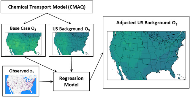
Graphical Abstract

1.0. INTRODUCTION

In the United States (US), ozone (O₃) is regulated as a criteria pollutant due to its ubiquitous nature and adverse impacts on human health and ecosystems. The National Ambient Air Quality Standard (NAAQS) for O₃ is currently set at a level of 70 ppb and was recently tightened from 75 ppb in 2015. In its recent reviews of the O₃ NAAQS, the US Environmental Protection Agency (EPA) noted the importance of background O₃,^1-4 that is the O₃ that would be present in the absence of anthropogenic emissions. Here, we focus on US background (US-B) O₃ which is defined as the O₃ that would exist if US anthropogenic (US-A) emissions were zero. Sources that lead to US-B O₃ include non-US anthropogenic pollution, wildfires, biogenic emissions, oxides of nitrogen (NO_X) from soil and lightning, stratosphere-to-troposphere exchange, and oxidation of global methane. As anthropogenic emissions decline and as the O₃ NAAQS is tightened, the portion of the O₃ leading to potential exceedances of the standard attributable to US-B O₃ increases.

US-B O₃ cannot be observed.^1-9 It is typically quantified using a chemical transport model (CTM). The most common approach is the zero-out method in which US-A emissions are set to zero. Since it is hypothetical, US-B O₃ estimates cannot be directly evaluated through comparison to observations. Some remote monitoring sites exist, but these are limited and are potentially affected by long range transport of US-A emissions. Global scale CTMs, often with coarse resolution, were first used to quantify US-B O₃⁵ and are still used today. Increasingly, regional scale CTMs with lateral boundary conditions (LBCs) derived from global or hemispheric scale simulations are used to achieve finer resolution in US-B O₃ estimates.^{2, 4, 10-13} There is much uncertainty in estimating US-B O₃.^{7-9, 12, 14, 15} Many different models have been used to quantify US-B O₃, often providing estimates that differ significantly.^7-9 For regional models, the choice of LBCs can have over 10 ppb impact on seasonal mean O₃.¹⁶ Uncertainty in US-B O₃ also comes from model biases, which may arise due to potential errors in model process descriptions and/or inputs (e.g., emissions, meteorology, LBCs) and which may vary from one model to another. Jaffe et al.⁹ estimated that the typical uncertainty in model-estimated seasonal mean US-B O₃ is ±10 ppb. This uncertainty arises primarily from model biases and differences between model predictions of US-B O₃. This uncertainty was based on a qualitative review of US-B O₃ estimates, but a quantitative assessment has not been conducted.

Previous studies have applied bias correction techniques to US-B O₃ estimates. Lin et al.¹⁷ applied a bias correction to AM3-simulated US-B O₃: “For each day, at all sites where AM3 overestimates observed MDA8 O₃ and where the estimated stratospheric contribution exceeds the model bias, [it was] assumed that the bias is caused entirely by excessive stratospheric O₃.” This method applies to one physical process and corrects bias on days with high stratospheric contributions to ground-level O₃. Dolwick et al.¹² adjusted US-B O₃ by scaling US-B O₃ by the ratio of observed O₃ to simulated total O₃. This method contains an inherent assumption that model biases in total O₃ translate proportionately to US-B and US-A O₃. That is, there is some source of bias in the model that affects all O₃ uniformly regardless of whether its origin is natural or anthropogenic. Neither of these methods treat biases arising from US-B O₃ and those arising from US-A sources separately.

We aim to fill two needs towards better characterizing US-B O₃. We develop a method to reduce the discrepancies between different estimates of US-B O₃, thus leading to improved agreement of an ensemble of US-B O₃ estimates. This is accomplished by fusing simulated total and US-B O₃ with ground-based observations. We separately apportion the model bias as a function of space and time that is attributable to US-B O₃ and US-A O₃. This allows for the calculation of adjusted O₃ that better aligns with observations and, potentially, for elucidation of key influences of bias for these two components of ozone. We also use a new metric to quantify the degree to which US-B O₃ convergence and model error, two factors leading to uncertainty in US-B O₃ estimation, are affected by the application of the data fusion adjustment method.

2.0. METHODS

2.1. Chemical Transport Model and Simulations.

We use a regional CTM, the Community Multiscale Air Quality (CMAQ) modeling system version 5.2.1,¹⁸ to simulate air quality over the contiguous US and parts of Mexico, Canada, and the Caribbean at 36km resolution for 2017. A sensitivity case for 2016 is also described below. For 2017, we simulate a base case in which all emission sources are included and a background case in which US anthropogenic emissions are removed while other emissions are identical to the base case. Meteorology is developed by application of the Weather Research Forecasting (WRF) Model¹⁹ version 3.8 using North American Regional Reanalysis²⁰ fields and observational data^{21, 22} to nudge WRF towards observations. WRF outputs are processed by the Meteorology-Chemistry Interface Processor²³ for use in CMAQ. Emissions are from the US EPA 2011 National Emissions Inventory (NEI) Emissions Modeling Platform version 3.²⁴ This platform includes projections of 2017 emissions that incorporate estimates of the impacts of current regulations. Detailed information on the projections for each emission sector is available in the Technical Support Document.²⁴ Projected emissions were replaced with year-specific emissions for electric generating unit sources based on continuous emissions monitoring system data and for fires. Emissions included in the background case are non-controllable O₃ sources as defined in Jaffe et al.⁹ These include non-US sources, lightning, biogenics, soil NO_X, wildfires, global methane, and stratosphere-to-troposphere transport. Lightning NO_X is simulated using an inline parameterization in CMAQ.²⁵ Biogenic VOC and soil NO_X are estimated using the Biogenic Emission Inventory System (BEIS). Wind-blown dust and sea salt emissions are estimated by inline CMAQ modules.^{26, 27} Wildfires are from the 2017 NEI.²⁸ Methane is set at a fixed value (1850 ppb). Stratospheric O₃ is parameterized in CMAQ as described below. For sources like soil NO_X, the entire source is allocated to US-B even though a portion is from anthropogenic nitrogen deposition and soil fertilization. Similarly, global methane includes US-A emissions. This highlights the complexity in US-B and US-A separation.

For both the base and US-B cases for 2017, we generate two estimates of O₃ by using two different sets of LBCs. One set of LBCs is based on a static vertical profile distributed with CMAQv5.2.1; the other set are hourly dynamic LBCs obtained from archived output of a Hemispheric CMAQ (HCMAQ)²⁹ simulation performed as part of an experimental near real-time air quality modeling system.³⁰ The O₃ transported into the modeling domain can differ significantly between the two sets of LBCs, as can the concentrations of O₃ precursors (Figures S1-S3). For the static LBCs, O₃ at the surface is 30-35 ppb while O₃ at the top of the model is 70 ppb. For the HCMAQ LBCs, the annual mean surface and near-surface O₃ is lower than the static LBCs while annual mean O₃ in upper layers of the HCMAQ-derived LBCs is much higher (Figure S1-S3). HCMAQ utilizes a potential vorticity based scaling of model upper troposphere-lower stratosphere (UTLS) O₃ to represent the effects of stratosphere-troposphere exchange^{29, 31} resulting in higher and more realistic O₃ in the upper layers which compare more favorably with typical ozonesonde data than do the static LBCs. This feature was not activated for the experimental near real-time HCMAQ simulations performed between January 1 and May 25, 2017, and used in this study, which may lead to a negative bias of O₃ in the simulation using these LBCs during this time period, though this bias should be corrected by the data fusion step. For each set of LBCs, the base case maximum daily 8-hour average (MDA8) simulated O₃ is separated into US-B and US-A components. The US-B component is the MDA8 O₃ from the background case, and the US-A component is the difference between the base and background case MDA8 O₃. In this formulation, US-A O₃ represents the enhancement of MDA8 O₃ above the US-B O₃ due to US anthropogenic (i.e., controllable) emissions.

We also obtained simulated base and US-B O₃ estimates for 2016. A more detailed description of the 2016 modeling framework is available in Henderson et al.,³² though a brief description is provided here. The 2016 simulations also provide two estimates of US-B O₃. Unlike the 2017 results, these estimates are obtained not from different LBCs but from different model scales and resolutions. One set of estimates are from HCMAQ simulations at 108km resolution. The other set is from a continental-scale CMAQ simulation at 12km resolution which was nested within a 36km simulation that was nested within the HCMAQ simulation (Figure S4). The emissions for the 2016 simulations are from the 2016 emissions modeling platform.^{33, 34} We focus primarily on the 2017 simulations to develop the method and to test the sensitivity of the method to different formulations. The 2016 simulations are incorporated to examine similarities and differences in the results that arise from differences in model year, scale, and inputs. Additional differences between 2016 and 2017 simulations may arise from differences in model configurations. Continental-scale simulations for both years use the same version of CMAQ (v5.2.1) though with slightly different chemical mechanisms mostly affecting organic aerosol.³⁵ Additional details on emissions and model configurations for the 2016 and 2017 hemispheric and continental-scale simulations are provided in Tables S1-S2.

2.2. Ozone Fusion Model.

For each of the 2017 LBC cases and each of the 2016 model resolution cases, we use a multivariate ordinary least squares regression with observed O₃ to derive separate estimates of model bias attributable to US-B and US-A O₃. Observations are from the Air Quality System (AQS) database which also includes observational data from the Clean Air Status and Trends Network (CASTNET) that provides monitoring of O₃ mostly in rural areas that are less influenced by US-A emissions. We calculate the observed MDA8 O₃ for each day for each site and pair it with the modeled MDA8 O₃ for days when at least 18 hours of observational data are available to obtain 380,587 daily observation-model pairs for 2017 and 366,912 pairs for 2016 at 1,256 (2017) and 1,243 (2016) individual sites (Figure 1).

Figure 1.

Locations of observation sites included in the regression model for 2017. Observation sites for 2016 are not exactly the same but are similarly distributed spatially. CASTNET sites are denoted by orange squares.

The regression model (Equation 1) has the form of an adjustment factor (α) for each component that varies with space and time:

$$[O_3{]}_{observed}={\alpha }_{{}_{US-B}}(s,t)\ast [O_3{]}_{US-B}^{sim}+{\alpha }_{{}_{US-A}}(\text{s,t})\ast [O_3{]}_{US-A}^{sim}$$ (1)

Where:

$$\begin{gathered} {\alpha }_{US-B}(s,t)={\alpha }_{0,US-B}+{\alpha }_{X,US-B}\ast X+{\alpha }_{Y,US-B}\ast Y+{\alpha }_{Z,US-B}\ast Z \\ +{\alpha }_{sin,US-B}\sin \left(\frac{2\pi }{365}d\right)+{\alpha }_{cos,US-B}\cos \left(\frac{2\pi }{365}d\right) \\ {\alpha }_{US-A}(s,t)={\alpha }_{0,US-A}+{\alpha }_{X,US-A}\ast X+{\alpha }_{Y,US-A}\ast Y+{\alpha }_{Z,US-A}\ast Z \\ +{\alpha }_{sin,US-A}\sin \left(\frac{2\pi }{365}d\right)+{\alpha }_{cos,US-A}\cos \left(\frac{2\pi }{365}d\right) \end{gathered}$$

The other variables, (s, t), included in the regression to determine the adjustment factors are longitude (X), latitude (Y), elevation (Z), and day of the year (d) transformed to a sinusoidal form to account for the cyclical nature of O₃ production and to identify seasonally dependent biases. Each of these variables are normalized to zero mean and unit variance. The value of α for a particular grid cell on a particular day is calculated by substituting X, Y, Z, and d for that grid cell and day into the equation. The observations used to train the regression model oversample low elevations, the eastern US, and O₃ season. Thus, the variables must be normalized by the mean and standard deviation of the training data (Table S3) before the regression model is applied to the gridded CTM data. An adjustment factor for the base case O₃ is calculated as follows:

$${\alpha }_{base}=\frac{{\alpha }_{{}_{US-B}}(\text{s,t})\ast [O_3{]}_{US-B}^{sim}+{\alpha }_{{}_{US-A}}(\text{s,t})\ast [O_3{]}_{US-A}^{sim}}{[O_3{]}_{US-B}^{sim}+[O_3{]}_{US-A}^{sim}}$$ (2)

Adjustment factors are developed separately for each of the four simulation cases then applied to the CTM-modeled results to calculate gridded adjusted O₃ which fuse observations and simulations. The adjusted base case O₃ is the sum of the adjusted US-B and US-A components.

This is the first study that we are aware of to use this particular inverse modeling approach for background ozone. We have observational constraints on O₃, and we have modeled O₃ components whose effects (if it were possible to model them perfectly) should sum to the observations. Our approach uses a multiple linear regression with relatively few predictor variables to scale the modeled O₃ components such that error is reduced when comparing to the observations. Related approaches in the existing literature have combined land use regression (LUR) models with CTM data.^{36, 37} One of the ways our approach differs from typical LUR models is that we only use information about the point in space (X, Y, Z) and do not incorporate any specific land use variables, though such information is involved in the inputs to CMAQ. We have added a temporal component in the form of a sinusoidal function of day of year to account for seasonal biases in the CTM data. We have also separated the total pollutant concentration into separate components and correct for the bias in each component individually.

3.0. RESULTS AND DISCUSSION

3.1. Chemical Transport Model Evaluation.

We first evaluated the ability of the base case CTM simulations to reproduce observed MDA8 O₃ (Table 1). For the 2017 36km simulations, the performance of one LBC case is not obviously superior to the other. The HCMAQ LBC case has better normalized mean bias (NMB) but worse normalized mean error (NME) and Pearson correlation (r) compared to the static LBC case, likely at least in part due to the erroneous omission of the UTLS O₃ scaling in the HCMAQ simulation through May 25, 2017. A comparison of the performance by month (Table S6) shows that the correlation for the HCMAQ LBC case was improved starting in June, though the error was not improved, due, in part, to the tendency of the UTLS O₃ scaling to exacerbate positive biases during autumn.³¹ The performance of the 2016 simulations are better than for 2017, though the 108km HCMAQ performance is only slightly better than the 2017 36km simulations. The performance of the 2016 12km resolution simulations showed the best performance out of all simulations. For all simulations, CMAQ tended to be biased high at lower O₃ levels and biased low at higher O₃ levels (Figures S5-S6, Table S4). We attribute the better performance of the 2016 simulations relative to the 2017 simulations to the quality of the emissions. The 2017 emissions are based on projections from the 2011 NEI emissions modeling platform while the 2016 emissions are from the 2016 emissions modeling platform.^27,28 We expect that the 2016 emissions are more representative of the specific year than the 2017 emissions due to improvements in emission estimation methodologies, the additional work that has been conducted in quality assuring the 2016 emissions, and increased uncertainty introduced in projecting the 2011 emissions to 2017.

Table 1.

Performance statistics for 2016 and 2017 base case simulations. The horizontal grid resolution of each simulation is given in parentheses. Performance goals and criteria are from Emery et al.³⁸ A more comprehensive set of performance metrics are found in SI (Table S5) along with the equations used to calculate performance metrics.

	NMB (%)	NME (%)	r
2017 HCMAQ LBC (36km)	13.34	24.37	0.54
2017 Static LBC (36km)	15.08	20.96	0.60
2016 CMAQ (12km)	1.19	15.26	0.76
2016 HCMAQ (108km)	10.09	20.38	0.59
Performance Goal	<±5%	<15%	>0.75
Performance Criteria	<±15%	<25%	>0.50

3.2. Ozone Fusion Model Results.

Using the results of the regression with observed MDA8 O₃ (Table S8), we calculate adjusted base case O₃ and two components (US-A and US-B O₃). By design, due to the formulation of the regression, the application of the O₃ adjustment results in improved performance for base case O₃ for all simulations (Table S9). We compare the 2017 US-B O₃ estimates for each LBC case that we obtain directly from CMAQ and the adjusted US-B O₃ estimates for each LBC case that we obtain after applying the fusion bias adjustment. The adjusted US-B O₃ estimates have better agreement with each other than the unadjusted CTM US-B O₃ estimates (Figure 2). The agreement of the two estimates is improved from R²=0.33 for the original CTM results to R²=0.70 for the adjusted results. We introduce a metric to quantify both the convergence of US-B O₃ estimates and base case model error of an ensemble of US-B O₃ estimates (Equation 3) which we refer to as a convergence metric. Though it does not necessarily measure uncertainty, the metric does measure US-B O₃ convergence and total O₃ model performance which are two factors affecting uncertainty in US-B O₃ estimates.

Figure 2.

Comparisons of 2017 US-B O₃ for HCMAQ and static LBC cases from CTM simulations (left), from regression model in Equation 1 without meteorological variables (middle), and from regression model in Equation S1 with meteorological variables (right).

$$convergence=std\left(\frac{{\sum }_{j=1}^N\mid \frac{{\sum }_{j=1}^N[O_3{]}_{US-B_i}^j}{N}-[O_3{]}_{US-B_i}^j\mid +\mid [O_3{]}_{bas{e}_i}^j-[O_3{]}_{ob{s}_i}\mid }{N}\right)$$ (3)

Where:

i = daily simulation-observation pair

j = a particular US-B estimation method

N = the total number of US-B estimation methods (HCMAQ and static LBC cases here)

To further explain this metric, we find the absolute value of the difference between the mean of the daily US-B O₃ for all cases for a particular year and the US-B O₃ estimate for each of those cases for each daily model-site pair. This results in N different ΔUS-B O₃ vectors with elements i. We also find the model error for each base case for each daily model-site pair, resulting in N different error vectors with elements i. For each case, the ΔUS-B O₃ and error vectors are summed for each element i, and the mean of their sum for each daily model-site pair across N cases is calculated, resulting in a single vector with elements i. Finally, we calculate the standard deviation of this vector across all of the daily model-site pairs to arrive at the estimated US-B O₃ convergence for the ensemble. We have applied this metric to the daily US-B O₃, but it could alternatively be applied to other averaging periods such as the seasonal mean.

Using this method to quantify the US-B O₃ convergence, we achieve a 28% improvement in the convergence metric by applying the US-B O₃ adjustment. The convergence metric of the daily US-B O₃ estimate is improved from 8.0 ppb to 5.8 ppb (Table S11). We tested the sensitivity of the regression model to meteorology by adding the following additional variables: temperature anomaly, relative humidity, and cloud cover (Equation S1). The inclusion of meteorological variables in the regression model had little effect on the resulting adjusted O₃. Using the regression with meteorology, the convergence metric of the daily US-B O₃ estimate is 5.5 ppb, a 32% improvement compared to simulated results and 0.3 ppb better than without meteorological adjustment. Coefficients for the regression with meteorology are available in the SI (Table S10).

The performance of the regression models is further analyzed through cross-validation. Only the results for the 2017 simulations are presented here since those are the results used to test different formulations of the model. Cross-validation results for 2016 simulations are available in the SI (Tables S12-S13). Both random and spatial data withholding are used. For the random withholding, the data is subset into groups each containing 10% of the data. Each of the ten groups are withheld as test sets while the remaining 90% of the data provides the training set. With random tenfold cross-validation, the model shows no loss of predictive power as the mean R² from the cross-validation is no different from the R² obtained using the full dataset (Table 2). For the spatial withholding, monitoring sites are divided into nine groups based on their locations so that there are approximately the same number of datapoints in each group (Figure S8). With the spatial cross-validation, there is a decrease in R² for each case, and there is variation in the performance for the different test sets, as indicated by the wide confidence intervals (Table 2).

Table 2.

R² values and cross-validation analysis for each 2017 LBC case for regression models both with and without meteorological variables included in the regression. The R² values shown for the cross-validation analysis are the means across all of the test sets. The 95% confidence intervals are shown in parentheses for the cross-validation results. More comprehensive results are available in SI (Tables S12-S13).

	All data	Random cross- validation	Spatial cross- validation
2017 HCMAQ LBC (36km) without meteorological adjustment	0.45	0.45 (±0.01)	0.36 (±0.23)
2017 HCMAQ LBC (36km) with meteorological adjustment	0.53	0.53 (±0.01)	0.46 (±0.22)
2017 Static LBC (36km) without meteorological adjustment	0.46	0.46 (±0.01)	0.38 (±0.29)
2017 Static LBC (36km) with meteorological adjustment	0.53	0.53 (±0.01)	0.47 (±0.26)

We select the model without meteorological variable adjustment for further analysis. While the model with meteorological adjustment performs better for total O₃, as evidenced by the higher R², there is not much difference in the level of agreement of the two estimates (HCMAQ and static LBC cases) of 2017 US-B O₃ obtained by the two formulations (with and without meteorological adjustment). Since we are primarily focused on US-B O₃, for which the two regression formulations perform similarly, we choose the simpler model which only contains space and time variables (Equation 1) for further analysis. This does not mean that meteorology has no effect on US-B O₃. Rather, it is that much of the variation in US-B O₃ associated with meteorological variables is already captured by the CTM, itself, and the spatial and temporal variables.

3.3. Trends in Ozone Adjustments.

The adjustments to O₃ are shown as the difference (Δ) in the CMAQ-simulated and adjusted O₃. Delta is thus equivalent to (1-α) times the CMAQ-simulated O₃. Visualizations of the α values are provided in the SI. Across all scenarios, we find common temporal patterns in the US average O₃ adjustments (Figure 3). The US-B O₃ adjustments all have a sinusoidal pattern with troughs in spring and crests in fall. They are mostly centered around about zero, except for the 2017 static LBC case which is centered slightly above zero. This indicates that CMAQ tends to overestimate US-B O₃ for the static LBC case throughout the year, possibly because of inaccurate levels of O₃ and precursor pollutants transported in from the boundary compared to other cases whose LBCs account for the time-variation of hemispheric transport of pollutants. US-B O₃ in the static LBC case is systematically higher than the HCMAQ LBC case. One contributing factor is that the O₃ at the lateral boundaries is higher in the static LBC case compared to the HCMAQ LBC case at the middle layers of the model (Figure S1) which is expected to lead to increased vertical transport of O₃ to the surface in the static LBC case compared to the HCMAQ LBC case. The sinusoidal temporal trend in the US-B adjustment remains in the static LBC case, indicating that there may be something inherent to the model which causes US-B O₃ to be biased low in spring and high in fall, considering that the temporal trend cannot be explained by variation in the LBCs. The US average adjustments for base case O₃ follow similar temporal trends as US-B O₃.

Figure 3.

Difference (in ppb) of CMAQ-simulated and adjusted base case, US-B, and US-A O₃ for each simulation. Δ = [O₃]_simulated – [O₃]_adjusted = (1 – α)*[O₃]_simulated. The values are the daily averages of all model grid cells over the contiguous US.

There are also similarities among the temporal patterns of the US-A O₃ adjustments for each modeling scenario. In general, the value is positive, indicating that simulated US-A O₃ is biased high. The degree of US-A O₃ bias increases with coarser model resolutions. The 2016 12km case shows a relatively small bias in summer. The 2017 36km HCMAQ LBC case shows greater bias in spring and summer, while the 2016 108km case shows greater bias in spring, summer, and fall. The 2017 36km static LBC case shows comparable bias to the 12km case when averaged across the US, but this is because positive and negative biases cancel out (Figure 4) rather than because of lower absolute error. Positive biases in O₃ with coarser regional model resolutions have been reported previously.^{39, 40} Here we find that this bias is largely due to US-A O₃ while biases in US-B O₃ are not very dependent on model resolution.

Figure 4.

Annual average of O₃ adjustments for all cases. Max, min, and mean refer to the maximum, minimum, and mean values over the contiguous US. Δ = [O₃]_simulated – [O₃]_adjusted = (1 – α)*[O₃]_simulated.

The adjustments for all scenarios share some common spatial patterns (Figure 4). The annual average of the daily US-B O₃ adjustments show spatial variation. In the 2017 36km cases, there is a north-to-south pattern, with more positive biases in the south than the north. For the 2017 simulations, the simulated US-B O₃ is biased slightly high on average, but the seasonal results for this case (Figures S17-S20) illustrate that there is a substantial negative bias in winter and spring that likely results from the erroneous omission of the UTLS O₃ scaling in the HCMAQ simulation and a substantial positive bias during summer and autumn. This tendency for an overall positive bias may be partially because of the influence of US-A emissions on HCMAQ LBCs that are used in the base case and the US-B case. For the HCMAQ LBC case, there are likely some effects of US anthropogenic emissions on the US-B O₃ simulations due to hemispheric circulation of US pollution. This is not the case for the 2016 simulations in which the base case and US-B simulations are driven by different sets of LBCs which have been nested down from separate base and US-B case hemispheric simulations. The 2017 HCMAQ simulation from which the LBCs are derived also relies on a different emissions inventory, which likely affects the results. The 2016 US-B O₃ is biased low on average throughout the domain for both the 12km CMAQ and 108km HCMAQ cases. The 2016 HCMAQ simulations have a negative bias in the upper troposphere, most notably in spring,^{4, 32} which is also when we find the most negative bias in surface US-B O₃. HCMAQ has been shown to have negative bias in the upper troposphere, especially in spring.⁴¹ However, a comparison of seasonal ozone fluctuations from HCMAQ and several other global models against ozonesonde data over North America showed that HCMAQ performed similarly to most other models.¹⁶ Though we have primarily discussed the annual averages here, there are season-dependent biases such as those arising from the lack of UTLS O₃ scaling (Figures 3, S17-S20).

The US-A O₃ adjustments show more spatial variation and greater deviation from zero compared to the US-B O₃ adjustments. In all cases, we find negative bias of US-A O₃ in the western US, particularly at high elevations. In most of the eastern US we find that US-A O₃ is biased high, though the bias decreases with finer model resolution. Similarly, the low US-A O₃ bias in the western US is reduced with finer model resolution. This further supports our findings that the coarser resolution CMAQ simulations perform worse for US-A O₃ and are biased high, with an average overproduction (or under-destruction) of ozone of about 2 ppb. Though US-A O₃ is biased high in the eastern US and low in the western US, so the spatial variation is removed by averaging across the domain. The adjustments for base case O₃ indicate positive bias in the eastern US and negative bias in the western US. This is as one might expect given the spatial adjustments in the O₃ components and the relative importance of US-A O₃ in the eastern US and US-B O₃ in much of the western US. In addition to the analysis shown here which uses observed O₃ from all sites in the AQS database, we have also repeated the analysis using only CASTNET sites to test whether the results are similar when we use a sparser monitoring network that covers mostly rural areas. Detailed results of the CASTNET analysis are shown in the SI (Tables S17, Figures S35-S36). The findings are similar to those expressed here. The main difference is that the inferred positive biases for US-A O₃ in the eastern US are lower when only CASTNET sites are considered. Since most CASTNET sites are rural, some of the positive biases for US-A O₃ in urban areas are not picked up.

3.4. Implications.

As anthropogenic emissions decline and as the O₃ NAAQS is tightened, correctly characterizing US-B O₃ becomes increasingly important in air quality policymaking. Though it is a model construct, accurately accounting for US-B O₃ in model applications is key to understanding future emission levels needed to attain the standard and to knowing the portion of O₃ attributable to US-A emissions. Uncertainties in estimates of background pollution will remain due to uncertainties in space and time characterization of large-scale flow patterns, stratosphere-troposphere exchange, natural emissions, and changing global emissions. The data fusion method for adjusting US-B O₃ introduced here has the potential to reduce the uncertainty in US-B O₃ estimates. The adjusted 2017 US-B O₃ estimates show better agreement with one another than do the US-B O₃ estimates obtained directly from the CTM. Improved agreement leads to reduced ensemble variation and increased model skill, two contributors to uncertainty arising from differences in US-B O₃ estimated by different methods. The method is, however, sensitive to the formulation of the regression model. For example, splitting the US-B O₃ into components (e.g., international, natural, and stratospheric) may lead to changes in the inferred error attribution. Covariation of O₃ components can reduce the ability of the regression model to associate CTM bias with the components.

The data fusion method allows model bias to be attributed separately to US-B and US-A O₃ components. This can help illuminate the timing and causes of biases within the model and inform the planning of more targeted research to investigate specific causes of bias. For instance, we have identified a negative bias in spring for US-B O₃ which could be due to several factors including too little stratosphere-troposphere exchange, too little vertical mixing from upper layers to surface layers, insufficient vertical resolution in upper layers, and/or the inability of coarse-resolution CTMs to accurately maintain plumes during intercontinental transport.⁴² While model resolution affects interactions between sources and processes for both US-B and US-A O₃, we find US-A O₃ is more sensitive to resolution than US-B O₃. Modifying the processes within the model or separately accounting for more sources (i.e., US-B sources separately) may alter the regression-based bias attribution. Exploration of these effects is an area for further research.

We have used least squares regression in this work, but other approaches (e.g., generalized additive models or machine learning) for attributing model error to O₃ components are also of interest. While we have applied our data fusion method only to one model here, this work has potential to be used in multi-model ensemble estimates of US-B O₃ to bring the estimates of different models into better agreement with one another and therefore reduce uncertainty of the overall US-B O₃ estimates. Across the four estimates, we find annual mean CTM-simulated US-B O₃ ranging from 30-37 ppb with the spring mean ranging from 32-39 ppb. After applying the bias adjustment, we find annual mean US-B O₃ ranging from 32-33 ppb with the spring mean ranging from 37-39 ppb. These estimates are within the range of US-B O₃ estimated by other studies summarized by Jaffe et al.⁹ We only draw conclusions for CMAQ based on our work, but some of the findings related to model bias, such as negative bias in spring in the western US and positive biases in the summer, have been observed in GEOS-Chem as well.¹⁴ Positive biases in summer at rural sites in the eastern US have been reported for AM3,⁴³ though the spring negative biases that we find here are not present in AM3 due to high stratospheric influences simulated by AM3 during spring.¹⁷

REFERENCES

- 1.USEPA, Integrated Science Assessment (ISA) of Ozone and Related Photochemical Oxidants (Final Report, Feb 2013). U.S. Environmental Protection Agency, Washington, DC, EPA/600/R-10/076F. 2013. [Google Scholar]
- 2.USEPA, Policy Assessment for the Review of the Ozone National Ambient Air Quality Standards. U.S. Environmental Protection Agency, Washington, DC, EPA-452/R-14/006. 2014. [Google Scholar]
- 3.USEPA, Integrated Science Assessment (ISA) for Ozone and Related Photochemical Oxidants (Final Report). U.S. Environmental Protection Agency. Washington, DC. EPA/600/R-20/012. 2020. [Google Scholar]
- 4.USEPA, Policy Assessment for the Review of the Ozone National Ambient Air Quality Standards. U.S. Environmental Protection Agency, Washington, DC, EPA-452/R-20-001. 2020. [Google Scholar]
- 5.Fiore A; Jacob DJ; Liu H; Yantosca RM; Fairlie TD; Li Q, Variability in surface ozone background over the United States: Implications for air quality policy. 2003, 108, (D24), DOI: 10.1029/2003jd003855. [DOI] [Google Scholar]
- 6.Hemispheric Transport of Air Pollution (HTAP). Hemispheric Transport of Air Pollution 2010, Part A: Ozone and Particulate Matter. Task Force on Hemispheric Transport of Air Pollution. Dentener F, Keating T and Akimoto H (eds.). Air Pollution Studies, No. 17 Geneva: United Nations Economic Commission for Europe. 2010. [Google Scholar]
- 7.McDonald-Buller EC; Allen DT; Brown N; Jacob DJ; Jaffe D; Kolb CE; Lefohn AS; Oltmans S; Parrish DD; Yarwood G; Zhang L, Establishing Policy Relevant Background (PRB) Ozone Concentrations in the United States. Environmental Science & Technology 2011, 45, (22), 9484–9497 DOI: 10.1021/es2022818. [DOI] [PubMed] [Google Scholar]
- 8.Fiore AM; Oberman JT; Lin MY; Zhang L; Clifton OE; Jacob DJ; Naik V; Horowitz LW; Pinto JP; Milly GP, Estimating North American background ozone in U.S. surface air with two independent global models: Variability, uncertainties, and recommendations. Atmospheric Environment 2014, 96, 284–300 DOI: 10.1016/j.atmosenv.2014.07.045. [DOI] [Google Scholar]
- 9.Jaffe DA; Cooper OR; Fiore AM; Henderson BH; Tonnesen GS; Russell AG; Henze DK; Langford AO; Lin MY; Moore T, Scientific assessment of background ozone over the US: Implications for air quality management. Elementa-Sci. Anthrop. 2018, 6, 30 DOI: 10.1525/elementa.309. [DOI] [PMC free article] [PubMed] [Google Scholar]
- 10.Emery C; Jung J; Downey N; Johnson J; Jimenez M; Yarwood G; Morris R, Regional and global modeling estimates of policy relevant background ozone over the United States. Atmospheric Environment 2012, 47, 206–217 DOI: 10.1016/j.atmosenv.2011.11.012. [DOI] [Google Scholar]
- 11.Mueller SF; Mallard JW, Contributions of Natural Emissions to Ozone and PM2.5 as Simulated by the Community Multiscale Air Quality (CMAQ) Model. Environmental Science & Technology 2011, 45, (11), 4817–4823 DOI: 10.1021/es103645m. [DOI] [PubMed] [Google Scholar]
- 12.Dolwick P; Akhtar F; Baker KR; Possiel N; Simon H; Tonnesen G, Comparison of background ozone estimates over the western United States based on two separate model methodologies. Atmospheric Environment 2015, 109, 282–296 DOI: 10.1016/j.atmosenv.2015.01.005. [DOI] [Google Scholar]
- 13.Luo H; Astitha M; Rao ST; Hogrefe C; Mathur R, Assessing the manageable portion of ground-level ozone in the contiguous United States. Journal of the Air & Waste Management Association 2020, 70, (11), 1136–1147 DOI: 10.1080/10962247.2020.1805375. [DOI] [PMC free article] [PubMed] [Google Scholar]
- 14.Guo JJ; Fiore AM; Murray LT; Jaffe DA; Schnell JL; Moore CT; Milly GP, Average versus high surface ozone levels over the continental USA: model bias, background influences, and interannual variability. Atmos. Chem. Phys 2018, 18, (16), 12123–12140 DOI: 10.5194/acp-18-12123-2018. [DOI] [Google Scholar]
- 15.Huang M; Bowman KW; Carmichael GR; Lee M; Chai T; Spak SN; Henze DK; Darmenov AS; da Silva AM, Improved western U.S. background ozone estimates via constraining nonlocal and local source contributions using Aura TES and OMI observations. 2015, 120, (8), 3572–3592 DOI: 10.1002/2014jd022993. [DOI] [Google Scholar]
- 16.Hogrefe C; Liu P; Pouliot G; Mathur R; Roselle S; Flemming J; Lin M; Park RJ, Impacts of different characterizations of large-scale background on simulated regional-scale ozone over the continental United States. Atmos. Chem. Phys 2018, 18, (5), 3839–3864 DOI: 10.5194/acp-18-3839-2018. [DOI] [PMC free article] [PubMed] [Google Scholar]
- 17.Lin M; Fiore AM; Cooper OR; Horowitz LW; Langford AO; Levy II H; Johnson BJ; Naik V; Oltmans SJ; Senff CJ, Springtime high surface ozone events over the western United States: Quantifying the role of stratospheric intrusions. 2012, 117, (D21), DOI: 10.1029/2012jd018151. [DOI] [Google Scholar]
- 18.United States Environmental Protection Agency. (2018). CMAQ (Version 5.2.1) [Software]. Available from 10.5281/zenodo.1212601. [DOI] [Google Scholar]
- 19.Skamarock WC; Klemp J; Dudhia J; Gill DO; Barker D; Wang W; Powers JG, A Description of the Advanced Research WRF Version 3. 2008, 27, 3–27. [Google Scholar]
- 20.NCEP North American Regional Reanalysis (NARR). In Research Data Archive at the National Center for Atmospheric Research, Computational and Information Systems Laboratory: Boulder, CO, 2005. [Google Scholar]
- 21.NCEP ADP Global Surface Observational Weather Data, October 1999 - continuing. In Research Data Archive at the National Center for Atmospheric Research, Computational and Information Systems Laboratory: Boulder, CO, 2004. [Google Scholar]
- 22.NCEP ADP Global Upper Air Observational Weather Data, October 1999 - continuing. In Research Data Archive at the National Center for Atmospheric Research, Computational and Information Systems Laboratory: Boulder, CO, 2004. [Google Scholar]
- 23.Otte TL; Pleim JE, The Meteorology-Chemistry Interface Processor (MCIP) for the CMAQ modeling system: updates through MCIPv3.4.1. Geosci. Model Dev 2010, 3, (1), 243–256 DOI: 10.5194/gmd-3-243-2010. [DOI] [Google Scholar]
- 24.USEPA, Technical Support Document (TSD) Preparation of Emissions Inventories for the Version 6.3, 2011 Emissions Modeling Platform. 2016. [Google Scholar]
- 25.Kang D; Pickering KE; Allen DJ; Foley KM; Wong DC; Mathur R; Roselle SJ, Simulating lightning NO production in CMAQv5.2: evolution of scientific updates. Geosci. Model Dev 2019, 12, (7), 3071–3083 DOI: 10.5194/gmd-12-3071-2019. [DOI] [PMC free article] [PubMed] [Google Scholar]
- 26.Foroutan H; Young J; Napelenok S; Ran L; Appel KW; Gilliam RC; Pleim JE, Development and evaluation of a physics-based windblown dust emission scheme implemented in the CMAQ modeling system. Journal of Advances in Modeling Earth Systems 2017, 9, (1), 585–608 DOI: 10.1002/2016ms000823. [DOI] [PMC free article] [PubMed] [Google Scholar]
- 27.Gantt B; Kelly JT; Bash JO, Updating sea spray aerosol emissions in the Community Multiscale Air Quality (CMAQ) model version 5.0.2. Geosci. Model Dev 2015, 8, (11), 3733–3746 DOI: 10.5194/gmd-8-3733-2015. [DOI] [Google Scholar]
- 28.USEPA, 2017 National Emissions Inventory Technical Support Document. 2020.
- 29.Mathur R; Xing J; Gilliam R; Sarwar G; Hogrefe C; Pleim J; Pouliot G; Roselle S; Spero TL; Wong DC; Young J, Extending the Community Multiscale Air Quality (CMAQ) Modeling System to Hemispheric Scales: Overview of Process Considerations and Initial Applications. Atmos Chem Phys 2017, 17, 12449–12474 DOI: 10.5194/acp-17-12449-2017. [DOI] [PMC free article] [PubMed] [Google Scholar]
- 30.Eder B; Gilliam R; Pouliot G; Mathur R; Pleim J, Continuous, Near Real-Time Evaluation of Air Quality Models. Environmental Managers, A&WMA 2017, 1–6. [PMC free article] [PubMed] [Google Scholar]
- 31.Xing J; Mathur R; Pleim J; Hogrefe C; Wang J; Gan CM; Sarwar G; Wong DC; McKeen S, Representing the effects of stratosphere–troposphere exchange on 3-D O3 distributions in chemistry transport models using a potential vorticity-based parameterization. Atmos. Chem. Phys 2016, 16, (17), 10865–10877 DOI: 10.5194/acp-16-10865-2016. [DOI] [Google Scholar]
- 32.Henderson BH; Dolwick P; Jang C; Misenis C; Possiel N; Timin B; Eyth A; Vukovich J; Mathur R; Hogrefe C; Pouliot G; Appel KW; Brehme K, Hemispheric CMAQ Application and Evaluation for 2016. In 2018 CMAS Conference, 2018. [Google Scholar]
- 33.USEPA, Technical Support Document (TSD) Preparation of Emissions Inventories for the Version 7.1 2016 North American Emissions Modeling Platform. 2019. [Google Scholar]
- 34.USEPA, Technical Support Document (TSD) Preparation of Emissions Inventories for the Version 7.1 2016 Hemispheric Emissions Modeling Platform. 2019. [Google Scholar]
- 35.Murphy BN; Woody MC; Jimenez JL; Carlton AMG; Hayes PL; Liu S; Ng NL; Russell LM; Setyan A; Xu L; Young J; Zaveri RA; Zhang Q; Pye HOT, Semivolatile POA and parameterized total combustion SOA in CMAQv5.2: impacts on source strength and partitioning. Atmos. Chem. Phys 2017, 17, (18), 11107–11133 DOI: 10.5194/acp-17-11107-2017. [DOI] [PMC free article] [PubMed] [Google Scholar]
- 36.Akita Y; Baldasano JM; Beelen R; Cirach M; de Hoogh K; Hoek G; Nieuwenhuijsen M; Serre ML; de Nazelle A, Large Scale Air Pollution Estimation Method Combining Land Use Regression and Chemical Transport Modeling in a Geostatistical Framework. Environmental Science & Technology 2014, 48, (8), 4452–4459 DOI: 10.1021/es405390e. [DOI] [PubMed] [Google Scholar]
- 37.Wang M; Sampson PD; Hu J; Kleeman M; Keller JP; Olives C; Szpiro AA; Vedal S; Kaufman JD, Combining Land-Use Regression and Chemical Transport Modeling in a Spatiotemporal Geostatistical Model for Ozone and PM2.5. Environmental Science & Technology 2016, 50, (10), 5111–5118 DOI: 10.1021/acs.est.5b06001. [DOI] [PMC free article] [PubMed] [Google Scholar]
- 38.Emery C; Liu Z; Russell AG; Odman MT; Yarwood G; Kumar N, Recommendations on statistics and benchmarks to assess photochemical model performance. Journal of the Air & Waste Management Association 2017, 67, (5), 582–598 DOI: 10.1080/10962247.2016.1265027. [DOI] [PubMed] [Google Scholar]
- 39.Thompson TM; Selin NE, Influence of air quality model resolution on uncertainty associated with health impacts. Atmos. Chem. Phys 2012, 12, (20), 9753–9762 DOI: 10.5194/acp-12-9753-2012. [DOI] [Google Scholar]
- 40.Punger EM; West JJ, The effect of grid resolution on estimates of the burden of ozone and fine particulate matter on premature mortality in the USA. Air Quality, Atmosphere & Health 2013, 6, (3), 563–573 DOI: 10.1007/s11869-013-0197-8. [DOI] [PMC free article] [PubMed] [Google Scholar]
- 41.Itahashi S; Mathur R; Hogrefe C; Zhang Y, Modeling stratospheric intrusion and trans-Pacific transport on tropospheric ozone using hemispheric CMAQ during April 2010 – Part 1: Model evaluation and air mass characterization for stratosphere–troposphere transport. Atmos. Chem. Phys 2020, 20, (6), 3373–3396 DOI: 10.5194/acp-20-3373-2020. [DOI] [PMC free article] [PubMed] [Google Scholar]
- 42.Eastham SD; Jacob DJ, Limits on the ability of global Eulerian models to resolve intercontinental transport of chemical plumes. Atmos. Chem. Phys 2017, 17, (4), 2543–2553 DOI: 10.5194/acp-17-2543-2017. [DOI] [Google Scholar]
- 43.Lin M; Horowitz LW; Payton R; Fiore AM; Tonnesen G, US surface ozone trends and extremes from 1980 to 2014: quantifying the roles of rising Asian emissions, domestic controls, wildfires, and climate. Atmos. Chem. Phys 2017, 17, (4), 2943–2970 DOI: 10.5194/acp-17-2943-2017. [DOI] [Google Scholar]
Associated Data
This section collects any data citations, data availability statements, or supplementary materials included in this article.