Classification of intrauterine growth restriction at 34–38 weeks gestation with machine learning models

Abstract

Objective:

Intrauterine growth restriction (IUGR) is one of the most common causes of stillbirths. The objective of this study is to develop a machine learning model that will be able to accurately and consistently predict whether the estimated fetal weight (EFW) will be below the 10th percentile at 34+0–37 + 6 week’s gestation stage, by using data collected at 20 + 0 to 23 + 6 weeks gestation.

Methods:

Recruitment for the prospective Safe Passage Study (SPS) was done over 7.5 years (2007–2015). An essential part of the fetal assessment was the non-invasive transabdominal recording of the maternal and fetal electrocardiograms as well as the performance of an ultrasound examination for Doppler flow velocity waveforms and fetal biometry at 20 + 0 to 23 + 6 and 34 + 0 to 37 + 6 week’s gestation. Several predictive models were constructed, using supervised learning techniques, and evaluated using the Stochastic Gradient Descent, k-Nearest Neighbours, Logistic Regression and Random Forest methods.

Results:

The final model performed exceptionally well across all evaluation metrics, particularly so for the Stochastic Gradient Descent method: achieving a 93% average for Classification Accuracy, Recall, Precision and F1-Score when random sampling is used and 91% for cross-validation (both methods using a 95% confidence interval). Furthermore, the model identifies the Umbilical Artery Pulsality Index to be the strongest identifier for the prediction of IUGR – matching the literature. Three of the four evaluation methods used achieved above 90% for both True Negative and True Positive results. The ROC Analysis showed a very strong True Positive rate (y-axis) for both target attribute outcomes – AUC value of 0.771.

Conclusions:

The model performs exceptionally well in all evaluation metrics, showing robustness and flexibility as a predictive model for the binary target attribute of IUGR. This accuracy is likely due to the value added by the pre-processed features regarding the fetal gained beats and accelerations, something otherwise absent from previous multi-disciplinary studies. The success of the proposed predictive model allows the pursuit of further birth-related anomalies, providing a foundation for more complex models and lesser-researched subject matter. The data available for this model was a vital part of its success but might also become a limiting factor for further analyses. Further development of similar models could result in better classification performance even with little data available.

1. Introduction

Fetal growth restriction (FGR), for which intrauterine growth restriction (IUGR) is a practical but imprecise surrogate, is one of the most common causes of stillbirths [1] and one of the main reasons for induced preterm birth. However, the diagnosis of fetal jeopardy preceding stillbirth is still a major problem. Ultrasound, at 34 + 0 to 37 + 6 weeks gestation, has only modest results in predicting the fetus with an estimated weight (EFW) < 10th percentile [2]. As such, the hope is on a combination of novel biomarkers alongside ultrasound to detect small-for-gestational-age (SGA) fetuses [3]. Using a combination of biomarkers, clinical risk factors and 20-week ultrasound examinations is only associated with a moderate rate of predictive success; as the area under the curve (AUC) was 0.69. This being the average of the positive predictive value (32%) and negative predictive value (91%) [4].

New methods, such as artificial intelligence, are therefore being investigated to improve the diagnosis. One such example shows that for nuclear magnetic resonance (NMR) and mass spectroscopy on all metabolites on the umbilical cord blood serum, the AUC was then 0.91 [5].

Although increased strength of fetal movements and fetal hiccups are associated with decreased risks of stillbirth [6], the association of reduced fetal movements with IUGR is still too uncertain to be used for routine assessment of fetal wellbeing [7]. Interdisciplinary developments in this area may help to improve clinical outcome [8].

In the past decade, there has been a considerable increase in the presence of machine learning in medicine. Although still very much in its infancy, there have been very promising studies done on the efficacy of these complex models and algorithms in medicine [9,10] its unintended consequences are also noted [11]. One such model is the supervised-learning model, defined by the use of existing data to compare with the outcomes predicted by the model in question. This method often precedes methods involving pattern-recognition during the exploration of unknown areas in the research (e.g. Unsupervised Learning) [12]. As such, supervised learning provides a valuable foundation for the validation of the model, and a step towards new discoveries.

The primary objective of the study is to develop a machine learning model that will be able to accurately and consistently predict whether the intra-uterine growth restriction at the 34 + 0 to 37 + 6 week’s gestation stage would be below 10%. This will be done using available data for validation.

For this investigation we used the detailed and extensive data of the prospectively collected for the Safe Passage Study (SPS), a collaborative study of the effect of alcohol use during pregnancy [13] on stillbirths [14] and sudden infant deaths [15]. In addition to maternal socioeconomic and demographic data, fetal physiology which included maternal and fetal ECGs, fetal ultrasound examinations were collected at different periods during pregnancy. The data utilized in the development of this model was collected from participants in Cape Town, South Africa, between 2007 and 2015. The research done and the results found in these studies were used to contextualize the data for use in a model that could predict FGR - a well-researched data set to test against.

As there seems to be a close association between fetal movements and accelerations of the fetal heart rate [16], we decided to use accelerations as a proxy for fetal movements. System 8000, a computerized antenatal fetal heart rate (FHR) analysis system was used as a guideline to assess accelerations of the FHR [17]. Decelerations were further quantified by calculating the area under the contraction curve [18].

The medical field, in general, has many universally accepted ‘gold-standard’ indicators for various anomalies – the fields of Obstetrics and Gynecology included [19–21]. As such, an opening exists for the implementation of machine learning models to both utilize existing standards and to challenge them. Thus, it is a unique opportunity to create a model based on recent discoveries that, in themselves, challenge previous norms. Proving successful in this endeavour would then allow the exploration of potentially new correlations between the data available and birth-related anomalies.

Previous studies done with the goal of classifying the association between Doppler flow velocimetry results and asymmetric fetal growth have shown promise but with much need for improvement [22]. In the pursuit for improved accuracy, combinations of methods were introduced – such as the use of novel biomarkers with ultrasound [23]. Another such combination used Doppler velocimetry with biophysical profiling [24].

Most recently, a combination of machine learning techniques and heart rate features were integrated for IUGR diagnosis [25]. The study showed promising results for the integration of machine learning, achieving a classification accuracy of 91%.

2. Material and methods

Recruitment for the prospective Safe Passage Study (SPS) was done over 7.5 years [13]. An essential part of the fetal assessment was the non-invasive transabdominal recording of the maternal and fetal electrocardiograms (mECG, fECG) as well as the performance of an ultrasound examination for Doppler flow velocity waveforms and fetal biometry at 20 + 0 to 23 + 6 and 34 + 0 to 37 + 6 weeks gestation. The ECGs were recorded by the AN24 fetal Halter device (Monica Health Care, Nottingham. UK). It has previously been demonstrated that this device is extremely successful in recording the fECGs at 20 + 0 to 23 + 6 weeks gestation - with a success rate of 95.4% [22]. Dedicated ultrasonologists performed all the ultrasound examinations according to a strict protocol. Fetal biometry included head circumference, biparietal diameter, abdominal circumference and femur length. Hadlock’s formula was used to calculate the EFW from the biometric measurements [23]. The mECGs and fECGs were collected for all participants, but ultrasound examinations (for biometry and Doppler) were limited to a subgroup of 28% of participants due to the heavy workload of obtaining this information in all participants. The subgroup was selected by randomization at 20 + 0 to 23 + 6 week’s gestation.

For the purposes of building a predictive model, two datasets were isolated from the original master set: one with data processed and collected from the heart rate data collected via the Monica AN24 fetal monitoring device, and the other isolated from the pre-existing dataset on maternal and fetal data (Table 1). These two datasets were then prepared and analysed using a combination of Jupyter [24] and Orange Data Mining Software [25] (see Table 2).

Table 1.

Table summarising each dataset used. Note, titles of datasets exist only to assist referencing and do not necessarily denote the information within.

Dataset Title:	Week20_ONLY
Source:	Academic Dataset
Dimensions:	4764 row × 14 columns
Brief Description:	This dataset contains the information collected from mothers and their fetuses at 20–24 weeks gestational age. This data has been processed from ECG data collected via the Monica AN24 Device. Originally processed by Ivan Calitz Crockart (2019).
Dataset Title:	F3
Source:	Academic Dataset
Dimensions:	2767 rows × 5 columns
Brief Description:	This dataset contains the information collected from mothers and their fetuses at 34+0–37 + 6 weeks gestational age. The data represents information pertaining to the health of the mother and the fetus at this stage - measuring the pulsality indexes of several arteries as well as intrauterine growth restriction as assessed by the estimated fetal weight.

Table 2.

Feature overview with a brief description of each feature present in the respective datasets. Week20_ONLY referring to a gestational age of 20 + 0 to 23 + 6 weeks, and F3 to 34 + 0 to 37 + 6 weeks.

Feature	Data Type	Description
Week20_ONLY nGB	Numerical	The number of times gained beats were recorded for the maternal heart rate
total_GB	Numerical	The sum of all the gained beats recorded for the maternal heart rate
GBoverTime(per hour)	Numerical	Ratio of the total gained beats recorded per hour of heart rate recording for the maternal heart rate
accDuration	Numerical	The total time (in seconds) of the entire recording that were recorded as accelerations for the maternal heart rate
totalDuration	Numerical	The total time (in seconds) of the recording for the maternal heart rate
nLB	Numerical	The number of times lost beats were recorded for the maternal heart rate
total_LB	Numerical	The sum of all the lost beats recorded for the maternal heart rate
nfGB	Numerical	The number of times gained beats were recorded for the fetal heart rate
total_fGB	Numerical	The sum of all the gained beats recorded for the fetal heart rate
fGBoverTime(per hour)	Numerical	Ratio of the total gained beats recorded per hour of heart rate recording for the fetal heart rate
fAccDuration	Numerical	The total time (in seconds) of the entire recording that were recorded as accelerations for the fetal heart rate
fTotalDuration	Numerical	The total time (in seconds) of the recording for the fetal heart rate
f_nLB	Numerical	The number of times lost beats were recorded for the fetal heart rate
total_fLB	Numerical	The sum of all the lost beats recorded for the fetal heart rate
F3
F3_UMBILICAL_ARTERY_PI	Numerical	The Pulsality Index (PI) value for the Umbilical Artery
F3_AVG_UTERINE_ARTERY_PI	Numerical	The average Pulsality Index (PI) value for the Uterine Artery
F3_MCA_PI	Numerical	The Pulsality Index (PI) value for the Middle Cerebral Artery
F3_IUGR3	Categorical	Whether or not the Intrauterine Growth Restriction was less than 3%
F3_IUGR10	Categorical	Whether or not the Intrauterine Growth Restriction was less than 10%

2.1. Data analysis

The methodology of the project closely followed that of the CRISP-DM Methodology [26]. This required extensive research to be done regarding the model in the medical context, followed by the definition of the problem from a data mining perspective – the objective as described in the introduction. Each dataset was then analysed individually, the features categorised and a preliminary Analytics Base Table (ABT) constructed for each set. The ABT is a preliminary tabular outline of the dataset with respect to the variable to be predicted (known as the target variable). Following this, data quality reports were constructed (Tables 3, 4, and 5), detailing the quality of the data present in each set. The quality of the data was determined by the percentages present (null values considered to be ‘missing data’), as well as the deviation and cardinality of the data. These quality reports were separated into continuous and categorical feature sets, since each type has different quality identifiers.

Table 3.

The data quality report for the Week20_ONLY dataset.

	Count	%Miss.	Card.	Min	1st Qrt.	Mean	Median	3rd Qrt.	Max	Std Dev.
nGB	4764	0.00	39	0	3.00	8.9404	8.0	13.0	59.0	6.8574
total_GB	4764	0.00	3240	0	616.75	3003.7278	1817.0	4152.5	37044.0	3539.0984
GBoverTime(per hour)	4764	0.00	1603	0	684.75	3308.1258	2000.0	4570.0	43000.0	3899.0871
accDuration	4764	0.00	786	0	1550.00	1654.8328	1695.0	1860.0	4030.0	451.3060
totalDuration	4764	0.00	296	0	3130.00	3141.0569	3230.0	3360.0	9610.0	781.0597
nLB	4764	0.00	38	0	0.00	2.3573	1.0	3.0	60.0	4.1340
total_LB	4764	0.00	1161	0	0.00	575.6371	115.0	377.25	107698.0	2999.5273
nfGB	4764	0.00	42	0	9.00	14.3298	14.0	19.0	48.0	6.9648
total_fGB	4764	0.00	3388	0	1759.75	3462.5649	2813.0	4239.0	86965.0	3544.5789
fGBoverTime(per hour)	4764	0.00	1156	0	2040.00	4128.5980	3200.0	4800.0	176000.0	5998.3244
fAccDuration	4764	0.00	770	0	1460.00	1528.6576	1558.0	1660.0	3362.0	319.4827
fTotalDuration	4764	0.00	371	0	3100.00	3141.6913	3200.0	3330.0	7860.0	616.9372
f_nLB	4764	0.00	41	0	8.00	13.0126	12.0	18.0	40.0	7.3192
total_fLB	4764	0.00	3111	0	1184.00	2500.1064	2110.0	3296.25	45277.0	2084.3124

Table 4.

The data quality report for the continuous features of the F3 dataset.

	Count	%Miss.	Card.	Min	1st Qrt.	Mean	Median	3rd Qrt.	Max	Std Dev.
F3_UMBILICAL_ARTERY_PI	644	76.7	10	0.5	0.8	0.9003	0.9	1.0	1.4	0.1546
F3_AVG_UTERINE_ARTERY_PI	657	76.3	15	0.4	0.6	0.7441	0.7	0.8	1.8	0.2078
F3_MCA_PI	638	76.9	18	1.5	1.5	1.7566	1.7	2.0	2.7	0.3174

Table 5.

The data quality report for the categorical features of the F3 dataset.

	Count	% Miss.	Card.	Mode	Mode Freq.	Mode %	2nd Mode	2nd Mode Freq.	2nd Mode %
F3_IUGR3	429.0	49.1	2.0	0.0	419.0	97.6690	1.0	10	2.3310
F3_IUGR10	429	49.1	2.0	0.0	402.0	93.7063	1.0	27	6.2937

The data quality reports for each of the two datasets used (Tables 3–5) provided important information for further preparation. These reports were split into two tables (where necessary), one for the continuous features and one for the categorical features. The dataset represented in Table 3 only has continuous features and, as such, only required a single table for the data quality report. Since this dataset was the result of processed data, already having undergone its own preparation, it had no missing datapoints. The cardinality varied greatly, suggesting a good spread of data with little repetition. However, the most obvious issue present was found in the ‘Min’ column, showing that all features had a minimum at zero. This was due to the presence of zero values in the dataset, ultimately skewing the data. These zero values most likely appear instead of missing values that were not shown as ‘null’ values. For several of the features, such as those representing durations, a value of zero would imply no data should be available from the row at all – since if the duration of collection is zero no data collection took place.

In the case of the second dataset, several issues presented themselves clearly from the beginning. Most notably, the alarmingly high percentages of missing data throughout the dataset. This, along with the low Count values, suggested a fair amount of data preparation would be necessary to achieve a predictive model for the IUGR outcome.

Once the quality of each dataset had been assessed, the relationships were visualised to identify any issues or potential opportunities present in the data that may have been missed. The spread of the data was displayed and assessed via density graphs, allowing one to identify any skewness or proportionality anomalies. The shapes of these graphs were then tabulated (Table 6), focusing on the continuous data since the categorical data benefits very little from this analysis.

Table 6.

The tabulated results of the data visualization analysis.

Feature vs Density	Graph Shape
nGB	Unimodal (Skewed right)
total_GB	Exponential
GBoverTime (per hour)	Exponential
accDuration	Normal (Unimodal)
nfGB	Normal (Unimodal)
total_fGB	Exponential
fGBoverTime(per hour)	Exponential
fAccDuration	Normal (Unimodal)
totalDuration	Normal (Unimodal)
fTotalDuration	Normal (Unimodal)
nLB	Exponential
f_nLB	Multimodal/Skewed Right
total_LB	Exponential
total_fLB	Unimodal (Skewed Right)
F3_UMBILICAL_ARTERY_PI	Multimodal/Normal (Unimodal)
F3_AVG_UTERINE_ARTERY_PI	Unimodal (Skewed Right)
F3_MCA_PI	Normal (Unimodal)

The next step in preparing the predictive model was to analyse the covariance and the correlation between the features. This was done using a collection of scatter plot facet grids (Fig. 1), to easily compare the relationships between sets of features. During this step, the effect of the zero values on the data became clear, with ‘walls’ appearing on the scatter plots - subsequently skewing the data. This further supported the information displayed in the data quality reports, confirming the pro-found effect of the zero value datapoints. Additionally, these scatter plots provided visual feedback for potential clustering of values that could assist in the application of classification techniques further on in the process. Unfortunately, with the zero values still present in the data these scatter plots provided little information further.

Fig. 1.

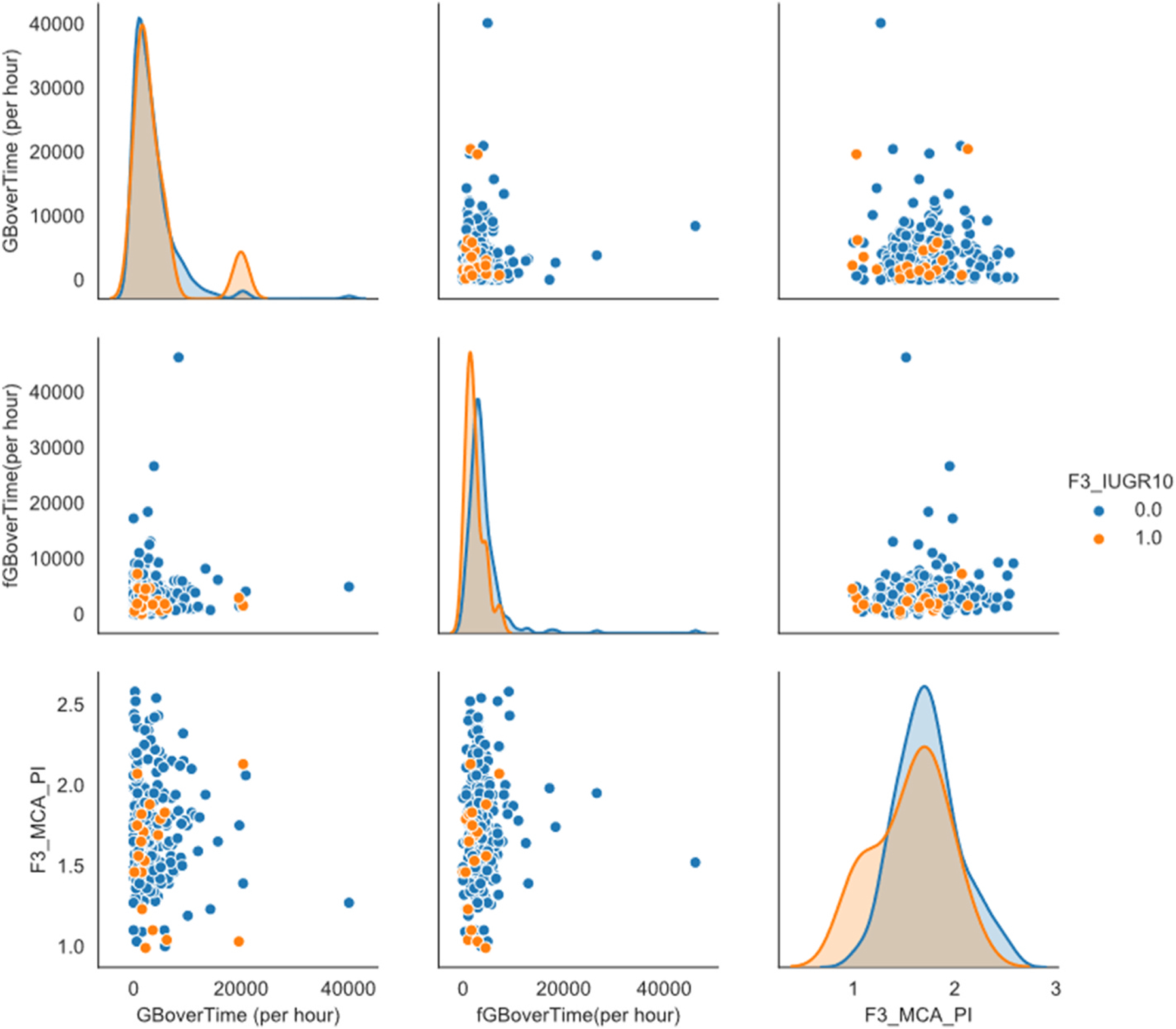
One of the scatter plot facet grids. This one compares the variables: GBoverTime(per hour), fGBoverTime(per hour) and F3_MCA_PI. Particular focus should be on the effect the ‘0′ values have on the data.

Once these steps were complete, a data quality plan was finalized (Table 7), outlining the issues found to be affecting the quality of the data for each feature. Included in this plan was a collection of potentially viable strategies to correct or mitigate the issues identified. Each feature was first analysed individually using the tables and reports previously generated, then analysed in relation to the other features. The most significant issues were identified – judged in accordance to their effect on the dataset as a whole. Once the issues were identified, potential solution strategies were then found for each issue – based on common industry practice and the aforementioned CRISP-DM approach. The potential strategies are tabulated, along with the issues and the corresponding feature, to be explored in a later stage of the process.

Table 7.

The Data Quality Plan in tabular form, giving a brief overview of the issues present and the handling strategies to be employed.

Feature	Data Quality Issue(s)	Potential Handling Strategies
Week20_ONLY nGB	Skew data	Remove rows with 0 values. Remove Outliers.
total_GB	Skew data/Outliers/High Cardinality	Remove rows with 0 values. Remove Outliers.
GBoverTime (per hour)	Skew data/Outliers	Remove rows with 0 values. Remove Outliers.
accDuration	Outliers (Low)	Remove rows with 0 values. Remove Outliers.
totalDuration	Outliers (Low)	Remove rows with 0 values. Remove Outliers.
nLB	Skew data/Outliers	Remove rows with 0 values. Remove Outliers.
total_LB	Skew data/Outliers	Remove rows with 0 values. Remove Outliers.
nfGB	Outliers (Low)	Remove rows with 0 values. Remove Outliers.
total_fGB	Skew data/Outliers/High Cardinality	Remove rows with 0 values. Remove Outliers.
fGBoverTime(per hour)	Skew data/Outliers	Remove rows with 0 values. Remove Outliers.
fAccDuration	Outliers (Low)	Remove rows with 0 values. Remove Outliers.
fTotalDuration	Outliers (Low)	Remove rows with 0 values. Remove Outliers.
f_nLB	Skewed data	Remove rows with 0 values. Remove Outliers.
total_fLB	Skewed data/High Cardinality	Remove rows with 0 values. Remove Outliers.
F3
f3_umbilical_artery_pi	Missing Data (76.7%)	Match metavalues (patID) to isolate relevant data
f3_avg_uterine_artery_PI	Missing Data (76.3%)	Match metavalues (patID) to isolate relevant data
f3_mca_pi	Missing Data (76.9%)	Match metavalues (patID) to isolate relevant data
f3_iugr3	Missing Data (49.1%)/Irregular Cardinality	Drop from dataset
f3_iugr10	Missing Data (49.1%)/Irregular Cardinality	Match metavalues (patID) to isolate relevant data

For all the features in the Week20_ONLY dataset, all issues seemed to be the result of the presence of the zero values mentioned earlier. As such, the removal of these invalid datapoints was designated as a potential solution strategy for all the features of this dataset. The features would then be assessed to determine the effectiveness of the strategy.

With the features of the F3 data, the extremely high percentage of missing values ruled out the use of imputation. As such, the first potential strategy was to merge the datasets by matching the patient ID’s in an attempt to isolate relevant data. For the categorical feature representing the presence of a 3% IUGR, it seemed best to remove it from the dataset as it became redundant once the target attribute had been chosen (F3_IUGR10).

2.2. Data preparation

Next, the data needed to be cleaned, removing any invalid datapoints – anything that would be read in by the software being used as ‘null’ or ‘NaN’ (Not a Number). This is vital in ensuring that the dataset is not contaminated with unnecessary or unknown datapoints. This process alone significantly reduced the available data of the F3 dataset (87% removed). Once the invalid data was removed, the outliers were identified using the covariance estimator method within Orange [25] – using a contamination value of 10%. Furthermore, any rows containing values of ‘0’ that would imply a null row (such as a totalDuration value of zero) were also removed. For the Week20_ONLY dataset the outlier identification removed 477 instances, while the removal of zeros reduced the available data from 4287 instances to 2611 instances – indicating a substantial amount of invalid datapoints present in the original data. The F3 dataset had no outliers removed and given the nature of the data, no invalid zero values were found or removed. At this point, the two datasets were merged, using the mutual meta-attribute ‘patID’. This ensured that the datasets were kept in context, matching the processed data with the data provided. The dataset had already been significantly reduced, but the remaining data would still prove valuable if prepared carefully.

After further study of the literature, the model was simplified by removing any values that pertain exclusively to the mother (i.e. maternal features). This is because the value of this data lies in what can be gleaned from the fetal features, an otherwise seldom-studied area.

Once cleaned, the data needed to be transformed to accommodate the modelling tools used later in the process. Given the disparity between the number of positive and negative values for the target attribute, sampling was introduced. The majority value (‘0’) was under-sampled – using only 20% of the data available, while the minority value (‘1’) was oversampled (80%). The two datasets produced from the sampling groups were then concatenated. Random sampling was later introduced as part of the evaluation, the data first undergoing normalization. For the preprocessing, the normalization method used standardized the set so that μ = 0 & σ = 1. After this the features were ranked according to Information Gain (Table 8).

Table 8.

A table displaying the feature rankings according the Orange’s ‘Rank’ method. Determined based on Information Gain and the Gain ratio.

	Info. gain	Gain ratio
fGBoverTime(per hour)	0.160	0.080
F3_UMBILICAL_ARTERY_PI	0.104	0.052
F3_AVG_UTERINE_ARTERY PI	0.088	0.044
f_nLB	0.072	0.036
fAccDuration	0.026	0.013
nfGB	0.026	0.013
F3_MCA_PI	0.010	0.005

Information Gain (formulae) [27]:

$$IG\left(S,X\right)=H\left(S\right)-\sum _{i=1}^N\left(\frac{|S_i|}{|S|}\cdot H\left(S_i\right)\right)$$

Where S denotes the set of training examples with i possible outcomes and X is the attribute that splits the set into subsets, S_i. H denotes the entropy.

Intrinsic value:

$$IV\left(S,X\right)=-\sum _{i=1}^N\frac{|T_i|}{|T|}\cdot \text{log}\left(\frac{|T_i|}{|T|}\right)$$

Information Gain Ratio:

$$IGR\left(S,X\right)=IG\left(S,X\right)/IV\left(S,X\right)$$

A Tree Model (Fig. 2) was used to determine which features were most informative and how they were used to predict the outcome of the target attribute. The first block present in the tree model informs us of the ratio of zero values to the total amount, the percentage this ratio represents and subsequently the feature that best defines the split that follows. Appearing above each of the subsequent blocks (one for each possible outcome) are the values of the feature that separate the groups. This served as a useful visualization of the classification of data within the current model. After observing the model, it becomes clear that accuracy could be improved by limiting a single feature over two ranges – namely, the feature representing the umbilical artery pulsality index. To validate this theory a ranking table was generated based on Information Gain (Table 8). According to the Tree Model, the Umbilical Artery PI alone strongly defined whether the IUGR value of the patient would fall below 10%. This is reaffirmed by the second-place ranking in Table 8. This result was a very important milestone in the process, because it validated the preliminary model when compared to the literature by ranking the umbilical artery pulsality index as the most informative standard feature (fGBoverTime(pe hour) being a constructed feature from the Week20_ONLY dataset) (see Fig. 3).

Fig. 2.

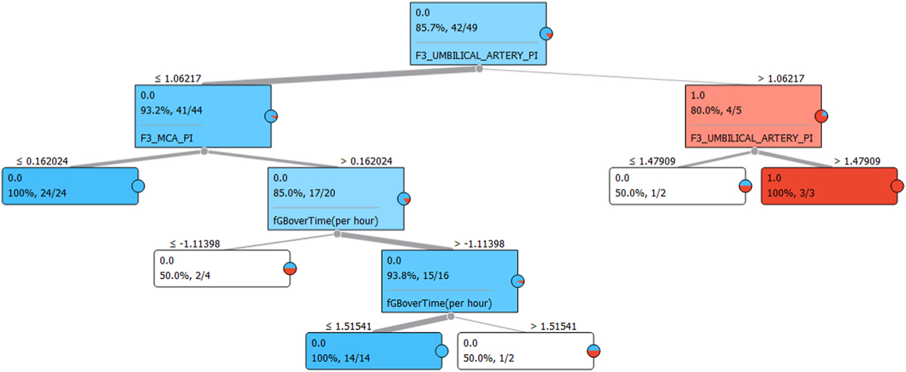
A screenshot of the Tree Model produced by Orange’s ‘Tree’ function.

Fig. 3.

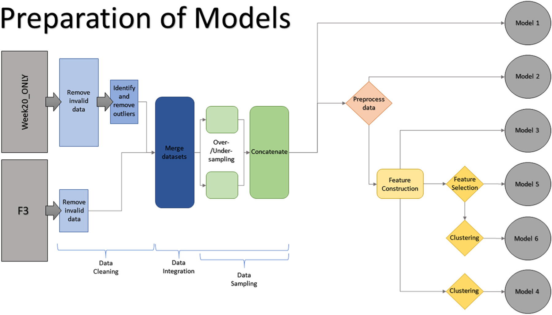
Graphical representation of the preparation process for each model.

Based on the abovementioned models and tables, two new categorical features are constructed:

• D1 for an Umbilical Artery PI value above 1.06217

• D2 for an Umbilical Artery PI value above 1.47909.

The features are then selected for the final model (Table 9).

Table 9.

The selected features and their types.

Name	Type
fGBoverTime(per hour)	Feature
fAccDuration	Feature
f_nLB	Feature
F3_UMBILICAL_ARTERY_PI	Feature
F3_AVG_UTERINE_ARTERY_PI	Feature
D1	Constructed Feature
D2	Constructed Feature
F3_IUGR10	Target Variable
patID	Meta Attribute

For the final phase of the data preparation a select set of features were chosen. These were selected based on the information gain rankings generated, as well as their contextual relevance regarding the desired outcome of the model. Two constructed features were added to the model, based on the information gained from the tree model (Fig. 2). The target variable, of course, had to be included as well as the meta attribute defining the method of merging.

3. Theory/calculation

Several baseline models were created at critical stages during the development of the predictive model, each was tested at these intervals to validate their effectiveness. These stages are outlined below:

• After Concatenation excluding Preprocessing (Model 1*)

• After Preprocessing without Feature Construction (Model 2*)

• After Feature Construction without Feature Selection (Model 3*)

• After Clustering without Feature Selection (Model 4*)

• After Feature Selection without Clustering (Model 5*)

• After Feature Selection + Clustering (Model 6*)

• Alternate Method - Without removing zero values

• Tested after Concatenation

• Tested after Preprocessing

To more accurately classify the data, Clustering - a process implemented to group otherwise abstract objects into classes - was attempted (Fig. 4). This was done via K-Means Clustering, and by subsequently producing distance values and feeding these into a Hierarchical Clustering method. Both methods were tested separately and in tandem, exploring the effect of the combined clustering methods on the model/dataset.

Fig. 4.

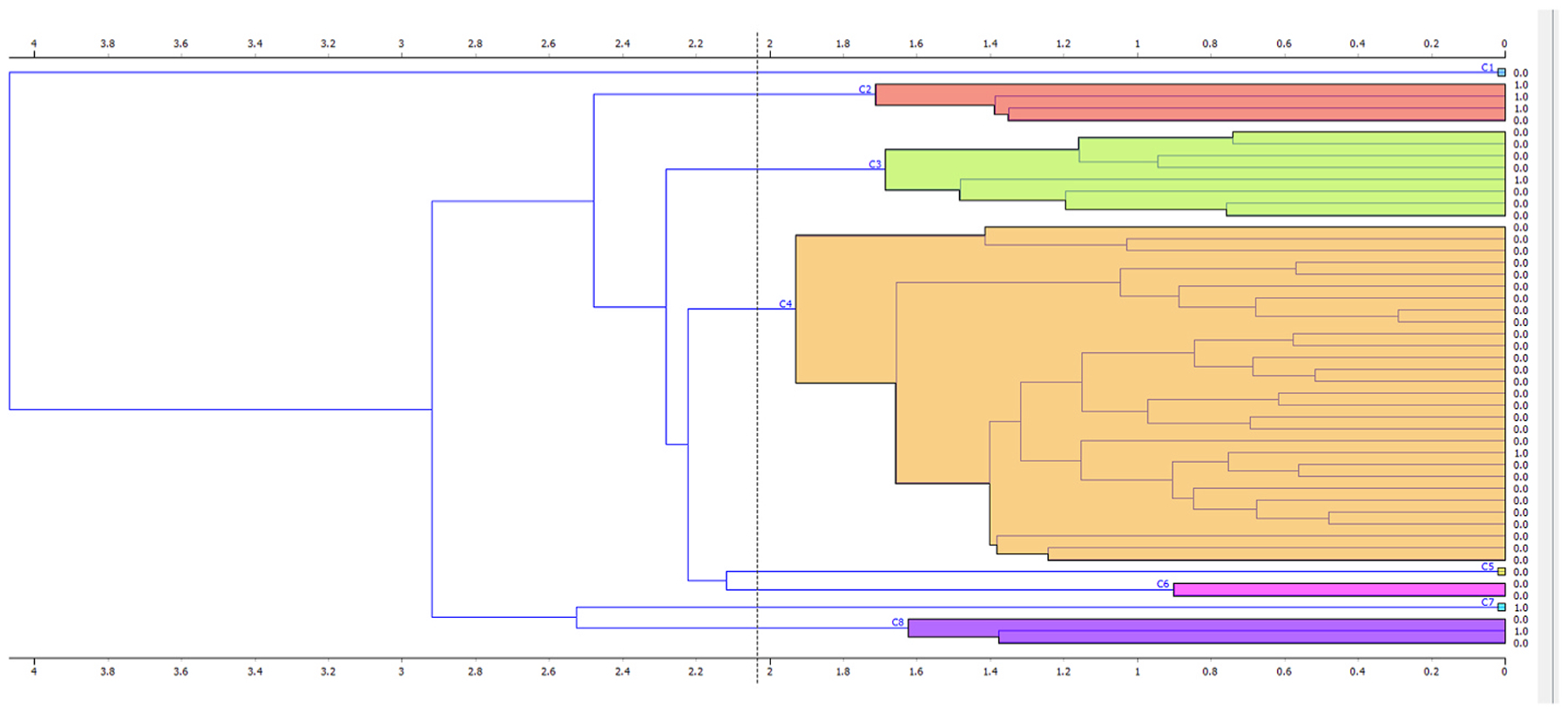
Visual results of the Hierarchical Clustering on the data. Average ‘Linkage’ used. Each colour represents a separate cluster of values.

Four testing methods are used to validate the performance of each model, chosen due to their near-mandatory presence in current literature as well as the variety they provide. It was important that the methods test the models’ effectiveness in all the relevant categories, ensuring the strengths and weaknesses were clearly highlighted.

3.1. Gradient Descent & regularization

To further model the data, Gradient Descent with Regularization [25] was used in its stochastic form. This was done to test and improve convergence of the algorithm by updating the relevant parameters of the model. Here, a hinge loss function was used for classification and a ‘squared ε insensitive’ loss function for regression. The regularization method was Ridge(L2) with a regularization strength (α) of 10⁻⁵. For the learning parameters, a constant learning rate (η₀) was used, initialized at 0.01.1000 iterations were used with a tolerance of 10⁻³. The data was then shuffled after each iteration to improve the objectivity of the method.

3.2. Logistic Regression & classification

Logistic Regression [25] is also implemented, both as a method of discrete classification and via the Gradient Method. Given the binary nature of the target attribute, Logistic Regression proves a good fit. The obstacle for this method was the imbalance present in the data regarding the number of negative and positive cases, this was tackled by the aforementioned sampling (20% under-sampling to 80% over-sampling). A Lasso(L1) regularization type is used with a strength value of C = 1.

3.3. Nearest Neighbour method

To further explore the effects of Clustering on the model/dataset, a Nearest Neighbour [25] method was setup and implemented. This method made use of distance values that were fed into a clustering method prior to evaluation. A Euclidean distance metric was chosen with the weighting based on distance values. A smaller k-value of 2 is used initially, but it was later found (after several iterations) that a larger value (5) produces a more optimal result.

3.4. Random Forest

The final method to be explored was the Random Forest method, implemented to take advantage of the clustering and classification methods used above. Particularly strong when correlation is weak, classification provides a potential solution for this. The probability of a correct prediction increases with the number of uncorrelated trees in our model [28]. Given the brevity of the tree model in Fig. 2, only 10 trees are used with subsets not being split past a value of 5. Replicable training was applied, and no individual depth limit was used.

4. Results

Several iterations were run for each of the 6 models defined in section 3; these iterations were used to optimise the values used for each of the algorithms and methods involved throughout the process. Such as those mentioned in section 3.

To quantify the performance of the predictive model a Test and Score function was used (Table 10). This compares the test data with the training data to evaluate the model as a learning algorithm. For one set of results random sampling was used, repeating 10 times per sample, with a training set size of 70%. To compare against, another set of results was produced using cross-validation with folding (3 folds were used here). Both methods made use of stratification and a 95% confidence interval. The results shown were averaged over both target attribute classes (i.e. 0 and 1). The AUC values of each of the models for each of the testing methods were condensed into two graphs (Figs. 5 and 6). These show how each model performed with regards to the AUC values and allowed easy visual verification for the selection of the final model. [29] To further explore the performance of the model, a Confusion Matrix was used (Table 11). Correctly classified positives are denoted as TP (True Positive), and incorrectly classified positives are denoted as FP (False Positive). Similarly, TN (True Negative) and FN (False Negative) were used in the evaluation. The Receiver Operating Characteristic (ROC) curves (Figs. 7 and 8) display the TP rate against the FP rate, a measure of the model’s ability to distinguish between classes.

Table 10.

The evaluation results for each model as produced by Orange’s ‘Test and Score’ function. Both sampling methods are included. The results shown are attained using a 95% confidence interval, inherent in the software function.

	Model 1 - Random Sampling(10, 70%); Stratified
Method	AUC	CA	F1	Precision	Recall
SGD	0.544	0.833	0.812	0.797	0.833
Random Forest	0.754	0.907	0.889	0.904	0.907
Logistic Regression	0.547	0.813	0.777	0.745	0.813
kNN	0.745	0.873	0.872	0.871	0.873
	Model 1 - Cross Validation(3 folds); Stratified
Method	AUC	CA	F1	Precision	Recall
SGD	0.607	0.878	0.856	0.859	0.878
Random Forest	0.639	0.898	0.872	0.909	0.898
Logistic Regression	0.561	0.857	0.791	0.735	0.857
kNN	0.779	0.816	0.821	0.827	0.816
	Model 2 - Random Sampling(10, 70%); Stratified
Method	AUC	CA	F1	Precision	Recall
SGD	0.544	0.833	0.812	0.797	0.833
Random Forest	0.668	0.853	0.818	0.803	0.853
Logistic Regression	0.738	0.833	0.818	0.806	0.833
kNN	0.492	0.800	0.785	0.771	0.800
	Model 2 - Cross Validation(3 folds); Stratified
Method	AUC	CA	F1	Precision	Recall
SGD	0.607	0.878	0.856	0.859	0.878
Random Forest	0.692	0.918	0.904	0.925	0.918
Logistic Regression	0.823	0.878	0.856	0.859	0.878
kNN	0.575	0.796	0.781	0.769	0.796
	Model 3 - Random Sampling(10, 70%); Stratified
Method	AUC	CA	F1	Precision	Recall
SGD	0.746	0.927	0.917	0.926	0.927
Random Forest	0.692	0.907	0.896	0.898	0.907
Logistic Regression	0.732	0.907	0.893	0.899	0.907
kNN	0.578	0.827	0.801	0.782	0.827
	Model 3 - Cross Validation(3 folds); Stratified
Method	AUC	CA	F1	Precision	Recall
SGD	0.774	0.918	0.913	0.913	0.918
Random Forest	0.833	0.898	0.886	0.888	0.898
Logistic Regression	0.803	0.898	0.886	0.888	0.898
kNN	0.590	0.837	0.825	0.817	0.837
	Model 4 - Random Sampling(10, 70%); Stratified
Method	AUC	CA	F1	Precision	Recall
SGD	0.746	0.927	0.917	0.926	0.927
Random Forest	0.739	0.907	0.893	0.899	0.907
Logistic Regression	0.732	0.907	0.893	0.899	0.907
kNN	0.578	0.827	0.801	0.782	0.827
	Model 4 - Cross Validation(3 folds); Stratified
Method	AUC	CA	F1	Precision	Recall
SGD	0.774	0.918	0.913	0.913	0.918
Random Forest	0.779	0.918	0.904	0.925	0.918
Logistic Regression	0.803	0.898	0.886	0.888	0.898
kNN	0.590	0.837	0.825	0.817	0.837
	Model 5 - Random Sampling(10, 70%); Stratified
Method	AUC	CA	F1	Precision	Recall
SGD	0.771	0.933	0.926	0.932	0.933
Random Forest	0.707	0.927	0.917	0.926	0.927
Logistic Regression	0.762	0.920	0.908	0.919	0.920
kNN	0.812	0.873	0.830	0.849	0.873
	Model 5 - Cross Validation(3 folds); Stratified
Method	AUC	CA	F1	Precision	Recall
SGD	0.774	0.918	0.913	0.913	0.918
Random Forest	0.816	0.898	0.886	0.888	0.898
Logistic Regression	0.789	0.918	0.913	0.913	0.918
kNN	0.867	0.878	0.836	0.893	0.878
	Model 6 - Random Sampling(10, 70%); Stratified
Method	AUC	CA	F1	Precision	Recall
	Model 1 - Random Sampling(10, 70%); Stratified
Method	AUC	CA	F1	Precision	Recall
SGD	0.771	0.933	0.926	0.932	0.933
Random Forest	0.707	0.927	0.917	0.926	0.927
Logistic Regression	0.762	0.920	0.908	0.919	0.920
kNN	0.812	0.873	0.830	0.849	0.873
	Model 6 - Cross Validation(3 folds); Stratified
Method	AUC	CA	F1	Precision	Recall
SGD	0.774	0.918	0.913	0.913	0.918
Random Forest	0.816	0.898	0.886	0.888	0.898
Logistic Regression	0.789	0.918	0.913	0.913	0.918
kNN	0.867	0.878	0.836	0.893	0.878

Fig. 5.

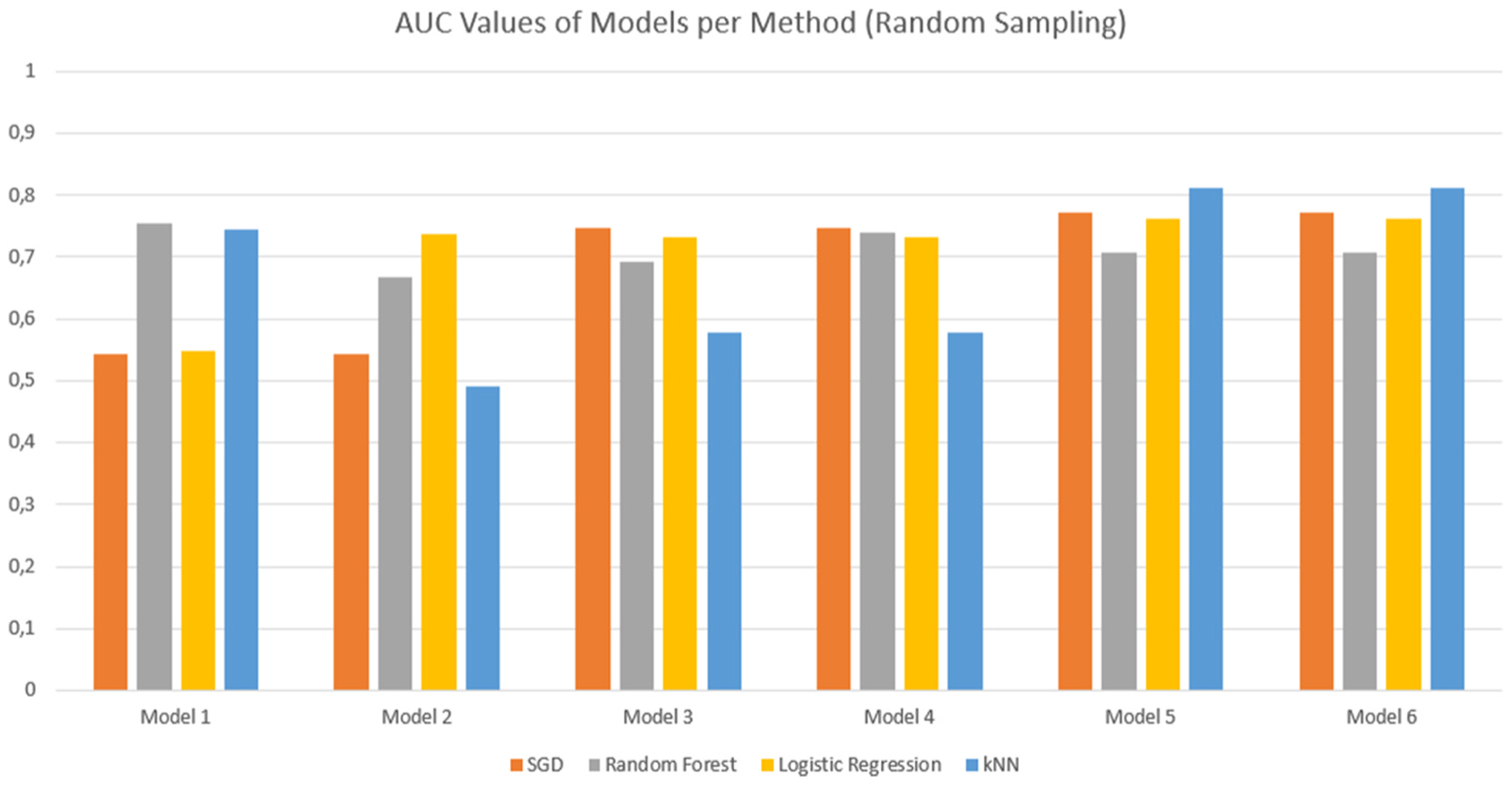
Comparative bar graph showing the AUC values for the different models for each evaluation method. These results were obtained using Random Sampling with Stratification.

Fig. 6.

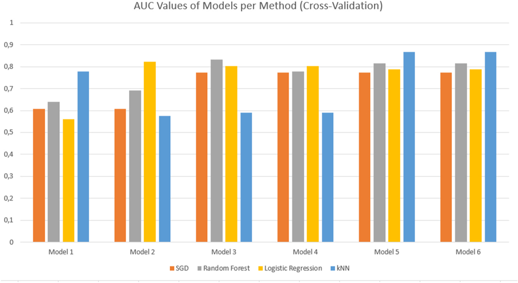
Comparative bar graph showing the AUC values for the different models for each evaluation method. These results were obtained using Cross Validation with Stratification.

Table 11.

Table showing the summarised Confusion Matrix results for each method used for the final model. The results are displayed as a percentage of the total number of predictions. The values highlighted in green represent the True values (desirable values), while those in red represent False values (undesirable values). [COLOUR].

KNN
	Predicted
Actual		0.0	1.0
	0.0	87.8%	33.3%	130
	1.0	12.2%	66.7%	20
		147	3	150
Logistic Regression
	Predicted
Actual		0.0	1.0
	0.0	92.1%	10.0%	130
	1.0	7.9%	90%	20
		140	10	150
Random Forest
	Predicted
Actual		0.0	1.0
	0.0	92.8%	9.1%	130
	1.0	7.2%	90.9%	20
		139	11	150
Stochastic Gradient Descent (SGD)
	Predicted
Actual		0.0	1.0
	0.0	93.5%	8.3%	130
	1.0	6.5%	91.7%	20
		138	12	150

Fig. 7.

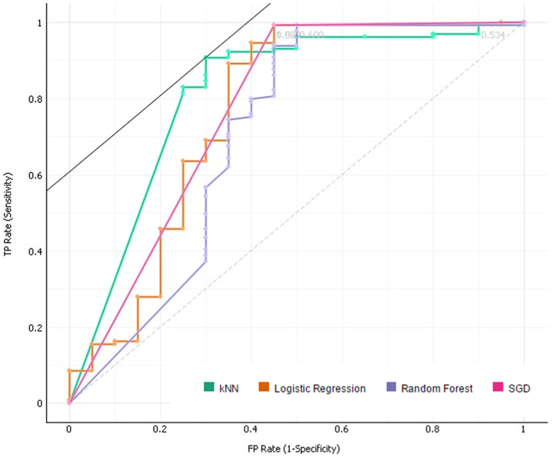
The resulting ROC curve for the final model. The curve shown is for Target Class ‘0’.

Fig. 8.

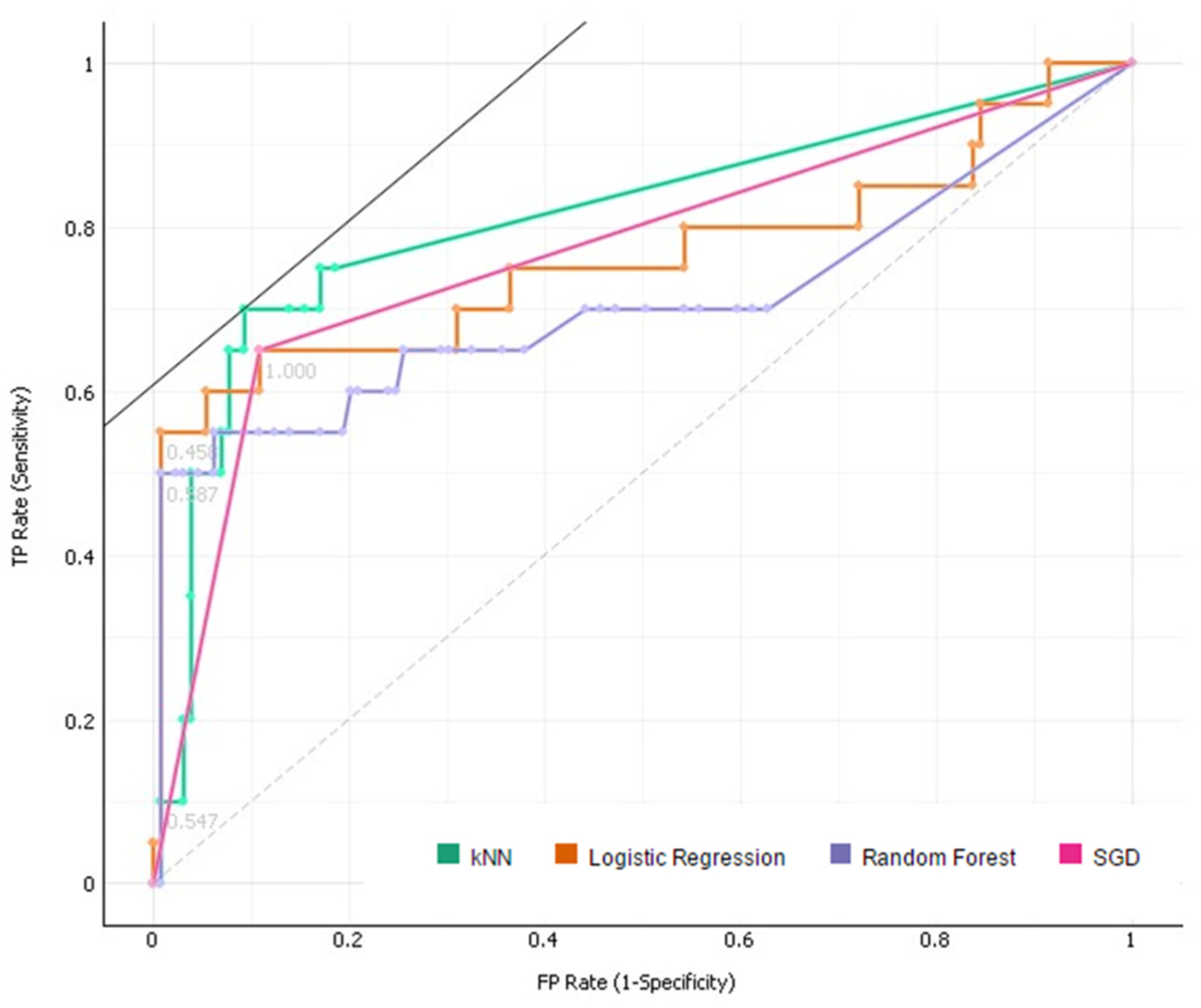
The resulting ROC curve for the final model. The curve shown is for Target Class ‘1’.

The evaluation of the model was done using 5 standard criteria:

Area under the ROC curve (AUC) – This method is independent of changes in the proportion of responders. It represents the area under the Receiver Operating Characteristic (ROC) curve. For a predictor f, an unbiased estimator of its AUC is expressed by the Wilcoxon-Mann-Whitney statistic [30].

$$AUC\left(f\right)=\frac{{\sum }_{t_0\in D^0}{\sum }_{t_1\in D^1}1\left[f\left(t_0\right)<f\left(t_1\right)\right]}{|D^0|\cdot |D^1|}$$

Where 1[f(t₀) < f(t₁)] denotes an indicator function; returning 1 iff the condition proves true, and 0 otherwise. D⁰ and D¹ represent the set of negative and positive examples, respectively.

Classification Accuracy (CA) - The proportion of the total number of predictions that were correct.

$$CA=\frac{TP+TN}{TP+TN+FP+FN}$$

F-score (F1) - The harmonic mean of Precision and Recall.

$$F1=2\left(\frac{\mathit{\text{Precision}}\times \mathit{\text{Recall}}}{\mathit{\text{Precision}}+\mathit{\text{Recall}}}\right)$$

Precision - The proportion of positive cases that were correctly identified.

$$\mathit{\text{Precision}}=\frac{TP}{TP+FP}$$

Recall - The proportion of negative cases which are correctly identified.

$$\mathit{\text{Recall}}=\frac{TP}{TP+FN}$$

The evaluation results were simplified into comparative bar graphs to better visualise the performance of each model (Figure(s) 4 & 5). Given that the AUC characteristic is a measure of the performance of the model in its classification of the dataset, this was chosen as the primary comparison metric. It is clear from the figures that models 5 and 6 perform the best in terms of their classification, although the two models seem to perform equally well. With little distinction between models 5 and 6 present, it was simply a matter of removing the redundant model. Cross-validation techniques proved more effective with regards to the AUC value obtained, with the models performing best under the kNN evaluation method.

5. Discussion

Our study confirms previous findings; that there is a strict correlation between umbilical Doppler velocimetry and IUGR [31]. However, there is still a need for improvement. In a recent study, a significant association was found between abnormal Doppler results and asymmetric fetal growth, but the sensitivity was low, 3.9% [32]. The authors concluded that maternal characteristics and imaging variables did not reliably identify more than one-third of pregnancies with evidence of suboptimal placentation.

Although there were concerns about missing data, much of it could be explained by the selection of a subgroup, consisting of 28% of the total group, as it would have been too expensive to do ultrasound examinations in all participants.

In our study, the pre-processed feature representing the fetal gained beats over time was ranked as most informative (Table 8), suggesting a strong correlation between the heart rate accelerations of the fetus and IUGR. The association of fetal movements with fetal heart rate changes was confirmed again, recently, when it was demonstrated that FHR accelerations synchronized with fetal movement bursts [33]. The combination of these results suggests significant predictive value in the inclusion of the gained beats and acceleration metrics, acting as more insightful features of the ECG data.

Although pregnant women observe a complex range of fetal movement patterns [34], it is difficult to quantify. As such, studies on fetal movement counting often do not provide sufficient evidence to influence practice [35]. Our better quantification of fetal movements by the determination of gained beats and the combination of different assessments of fetal wellbeing (such as fetal movement counts and Doppler velocimetry) likely contribute to our better identification of IUGR when compared to other studies.

The results of the Test and Score function are the most comprehensive regarding the overall performance of the model (Table 10). The best performing model achieving an F1 score of above 90% for all methods but k-Nearest Neighbours. The accuracy, precision and recall metrics all achieving above 90% for the SGD method, with only the AUC value being below this.

The Confusion Matrix (Table 11), a performance measurement tool for machine learning classification, serves as a simplified version of the evaluation table. This matrix shows the performance of the model in terms of classification accuracy. Three of the four evaluation methods used achieved above 90% for both True Negative and True Positive results. This is a significant result for any model, indicating an extremely high level of consistency and accuracy. The relatively poor performance shown by the kNN method indicates that this problem does not benefit as much from pattern recognition techniques.

The ROC Analysis (Figs. 7 and 8) that follows the evaluation, displaying the results for both Target Class cases, shows a very strong True Positive rate (y-axis) for both cases. The ROC curves represent the relationship between the sensitivity and the specificity of the algorithm. The area under the curve (represented by the AUC value) is equivalent to the probability that an arbitrary positive instance is ranked higher than an arbitrary negative instance. Although more valuable for classification problems, the AUC serves as a general metric for predictive accuracy.

The model performs exceptionally well in all evaluation metrics, showing robustness and flexibility as a predictive model for the binary target attribute of fetal growth restriction.

6. Conclusions

This paper discusses and explores the efficacy of the proposed model in the prediction of intrauterine growth restriction at the 34+0–37 + 6 week’s gestation age. Several predictive models were constructed using supervised learning techniques, and evaluated using the Stochastic Gradient Descent, k-Nearest Neighbours, Logistic Regression and Random Forest methods. The final model performed exceptionally well across all evaluation metrics, particularly so for the Stochastic Gradient Descent method: achieving a 93% average for Classification Accuracy, Recall, Precision and F1-Score when random sampling is used and 91% for cross-validation. This accuracy is likely due to the value added by the pre-processed features regarding the fetal gained beats and accelerations, something otherwise absent from previous multi-disciplinary studies. Furthermore, the model identifies the Umbilical Artery Pulsality Index to be the strongest identifier for the prediction of the Intra-Uterine Growth Restriction – matching the literature as the golden standard identifier.

In future, more techniques will be explored with a particular focus in optimizing the process. As more data becomes available and the models become more accurate and robust, deep learning techniques might be worth exploring. However, validatory studies such as this are vital steps in the early stages of the process.

The success of the proposed predictive model allows the pursuit of further birth-related anomalies, providing a foundation for more complex models and lesser-researched subject matter. The extensive data available for this model was a vital part of its success but might also become a limiting factor for further analyses when less data might be available. Further development of such models will allow for better performance with less data, improving the health and well-being of both mother and fetus.

References

- [1].Audette MC, Kingdom JC. Screening for fetal growth restriction and placental insufficiency. Semin Fetal Neonatal Med 2018;23(2):119–25. https://linkinghub.elsevier.com/retrieve/pii/S1744165X1730135X. [DOI] [PubMed] [Google Scholar]
- [2].Ciobanu A, Khan N, Syngelaki A, Akolekar R, Nicolaides KH. Routine ultrasound at 32 vs 36 weeks’ gestation: prediction of small-for-gestational-age neonates. Ultrasound Obstet Gynecol [Internet]. 2019. April 30;uog.20258, https://onlinelibrary.wiley.com/doi/abs/10.1002/uog.20258. [DOI] [PubMed] [Google Scholar]
- [3].Gaccioli F, Aye ILMH, Sovio U, Charnock-Jones DS, Smith GCS. Screening for fetal growth restriction using fetal biometry combined with maternal biomarkers. Am J Obstet Gynecol 2018;218(2). S725–37. https://linkinghub.elsevier.com/retrieve/pii/S0002937817324766. [DOI] [PubMed] [Google Scholar]
- [4].McCowan LME, Thompson JMD, Taylor RS, Baker PN, North RA, Poston L, et al. Prediction of small for gestational age infants in healthy nulliparous women using clinical and ultrasound risk factors combined with early pregnancy biomarkers. In: Gebhardt S, editor. PLoS one [internet]. vol. 12; 2017, e0169311. 1, https://dx.plos.org/10.1371/journal.pone.0169311. [DOI] [PMC free article] [PubMed] [Google Scholar]
- [5].Bahado-Singh RO, Yilmaz A, Bisgin H, Turkoglu O, Kumar P, Sherman E, et al. Artificial intelligence and the analysis of multi-platform metabolomics data for the detection of intrauterine growth restriction. In: Baud O, editor. PLoS one [internet]. vol. 14; 2019, e0214121. 4, https://dx.plos.org/10.1371/journal.pone.0214121. [DOI] [PMC free article] [PubMed] [Google Scholar]
- [6].Heazell AEP, Budd J, Li M, Cronin R, Bradford B, McCowan LME, et al. Alterations in maternally perceived fetal movement and their association with late stillbirth: findings from the Midland and North of England stillbirth case–control study. BMJ Open [Internet] 2018;8(7):e020031. http://bmjopen.bmj.com/lookup/doi/10.1136/bmjopen-2017-020031. [DOI] [PMC free article] [PubMed] [Google Scholar]
- [7].Imdad A, Yakoob MY, Siddiqui S, Bhutta Z. Screening and triage of intrauterine growth restriction (IUGR) in general population and high risk pregnancies: a systematic review with a focus on reduction of IUGR related stillbirths. BMC Public Health [Internet 2011;11(Suppl 3):S1. http://bmcpublichealth.biomedcentral.com/articles/10.1186/1471-2458-11-S3-S1. [DOI] [PMC free article] [PubMed] [Google Scholar]
- [8].Lai J, Nowlan NC, Vaidyanathan R, Shaw CJ, Lees CC. Fetal movements as a predictor of health. Acta Obstet Gynecol Scand [Internet] 2016;95(9):968–75. 10.1111/aogs.12944. [DOI] [PMC free article] [PubMed] [Google Scholar]
- [9].Gulshan V, Peng L, Coram M, Stumpe MC, Wu D, Narayanaswamy A, et al. Development and validation of a deep learning algorithm for detection of diabetic retinopathy in retinal fundus photographs. JAMA [Internet] 2016;316(22):2402. http://jama.jamanetwork.com/article.aspx?doi=10.1001/jama.2016.17216. [DOI] [PubMed] [Google Scholar]
- [10].Rajkomar A, Dean J, Kohane I. Machine learning in medicine. N Engl J Med 2019; 380(14):1347–58 [Internet], http://www.nejm.org/doi/10.1056/NEJMra1814259. [DOI] [PubMed] [Google Scholar]
- [11].Cabitza F, Rasoini R, Gensini GF. Unintended consequences of machine learning in medicine. J Am Med Assoc 2017;318(6):517 [Internet], http://jama.jamanetwork.com/article.aspx?doi=10.1001/jama.2017.7797. [DOI] [PubMed] [Google Scholar]
- [12].Deo RC. Machine learning in medicine. Circulation [Internet] 2015;132(20). 1920–30, https://www.ahajournals.org/doi/10.1161/CIRCULATIONAHA.115.001593. [DOI] [PMC free article] [PubMed] [Google Scholar]
- [13].Dukes KA, Burd L, Elliott AJ, Fifer WP, Folkerth RD, Hankins GDV, et al. The safe passage study: design, methods, recruitment, and follow-up approach. Paediatr Perinat Epidemiol 2014;28(5):455–65. 10.1111/ppe.12136 [Internet]. [DOI] [PMC free article] [PubMed] [Google Scholar]
- [14].Dukes K, Tripp T, Willinger M, Odendaal H, Elliott AJ, Kinney HC, et al. Drinking and smoking patterns during pregnancy: development of group-based trajectories in the Safe Passage Study. Alcohol 2017;62:49–60 [Internet], https://linkinghub.elsevier.com/retrieve/pii/S0741832917300113. [DOI] [PMC free article] [PubMed] [Google Scholar]
- [15].Elliott AJ, Kinney HC, Haynes RL, Dempers JD, Wright C, Fifer WP, et al. Concurrent prenatal drinking and smoking increases risk for SIDS: safe Passage Study report. EClinicalMedicine 2020;19:100247 [Internet], https://linkinghub.elsevier.com/retrieve/pii/S2589537019302561. [DOI] [PMC free article] [PubMed] [Google Scholar]
- [16].Sadovsky E, Rabinowitz R, Freeman A, Yarkoni S. The relationship between fetal heart rate accelerations, fetal movements, and uterine contractions. Am J Obstet Gynecol [Internet] 1984;149(2). 187–9, https://linkinghub.elsevier.com/retrieve/pii/0002937884901960. [DOI] [PubMed] [Google Scholar]
- [17].Dawes GS, Moulden M, Redman CWG. System 8000: computerized antenatal FHR analysis. J Perinat Med [Internet] 1991;19(1–2):47–51. https://www.degruyter.com/view/j/jpme.1991.19.issue-1-2/jpme.1991.19.1-2.47/jpme.1991.19.1-2.47.xml. [DOI] [PubMed] [Google Scholar]
- [18].Kieser E, Odendaal H, Van den Heever D. Development of a signal processing and feature extraction framework for the safe passage study. In: 2018 3rd biennial South African biomedical engineering conference (SAIBMEC) [internet]. IEEE; 2018. p. 1–4. https://ieeexplore.ieee.org/document/8363193/. [Google Scholar]
- [19].Poon LCY, Volpe N, Muto B, Yu CKH, Syngelaki A, Nicolaides KH. Second-Trimester uterine artery Doppler in the prediction of stillbirths. Fetal Diagn Ther 2013;33(1):28–35 [Internet], https://www.karger.com/Article/FullText/342109. [DOI] [PubMed] [Google Scholar]
- [20].Côté A-M, Firoz T, Mattman A, Lam EM, von Dadelszen P, Magee LA. The 24-hour urine collection: gold standard or historical practice? Am J Obstet Gynecol [Internet] 2008;199(6):625. e1–625.e6, https://linkinghub.elsevier.com/retrieve/pii/S0002937808006194. [DOI] [PubMed] [Google Scholar]
- [21].Honein MA, Paulozzi LJ. Birth defects surveillance: assessing the “gold standard”. Am J Public Health [Internet] 1999;89(8):1238–40. http://ajph.aphapublications.org/doi/10.2105/AJPH.89.8.1238. [DOI] [PMC free article] [PubMed] [Google Scholar]
- [22].Aditya I, Tat V, Sawana A, Mohamed A, Tuffner R, Mondal T. Use of Doppler velocimetry in diagnosis and prognosis of intrauterine growth restriction (IUGR): a Review. J Neonatal Perinat Med 2016;9(2):117–26 [Internet], https://www.medra.org/servlet/aliasResolver?alias=iospress&doi=10.3233/NPM-16915132. [DOI] [PubMed] [Google Scholar]
- [23].Geerts L, Van der Merwe E, Theron A, Rademan K. Placental insufficiency among high-risk pregnancies with a normal umbilical artery resistance index after 32 weeks. Int J Gynecol Obstet [Internet] 2016;135(1):38–42. 10.1016/j.ijgo.2016.03.038. [DOI] [PubMed] [Google Scholar]
- [24].Gaccioli F, Aye ILMH, Sovio U, Charnock-Jones DS, Smith GCS. Screening for fetal growth restriction using fetal biometry combined with maternal biomarkers. Am J Obstet Gynecol [Internet] 2018;218(2). S725–37, https://linkinghub.elsevier.com/retrieve/pii/S0002937817324766. [DOI] [PubMed] [Google Scholar]
- [25].Signorini MG, Pini N, Malovini A, Bellazzi R, Magenes G. Integrating machine learning techniques and physiology based heart rate features for antepartum fetal monitoring. Computer Methods and Programs in Biomedicine [Internet] 2020. March;185, https://www.sciencedirect.com/science/article/abs/pii/S0169260719308107?casa_token=YT1JkL8LrzYAAAAA:g4Y6LedwPUoRcDJU2lssLXoCAgevbu_IDlpLmV5uyV4vs7H7LQu6UzBHlwD4D3ZV8h5c59f-Ag. [DOI] [PubMed] [Google Scholar]
- [26].Hofmeyr F, Groenewald CA, Nel DG, Myers MM, Fifer WP, Signore C, et al. Fetal heart rate patterns at 20 to 24 weeks gestation as recorded by fetal electrocardiography. J Matern Neonatal Med [Internet] 2014;27(7):714–8. http://www.tandfonline.com/doi/full/10.3109/14767058.2013.836485. [DOI] [PMC free article] [PubMed] [Google Scholar]
- [27].Hadlock FP, Harrist RB, Sharman RS, Deter RL, Park SK. Estimation of fetal weight with the use of head, body, and femur measurements—a prospective study. Am J Obstet Gynecol [Internet] 1985;151(3):333–7. https://linkinghub.elsevier.com/retrieve/pii/0002937885902984. [DOI] [PubMed] [Google Scholar]
- [28].Jupyter. Jupyter - documentation [internet]. https://jupyter.org/documentation.
- [29].Metz CE. Basic principles of ROC analysis. Semin Nucl Med 1978;8(4):283–98. [DOI] [PubMed] [Google Scholar]
- [30].Demsar J, Curk T, Erjavec A, Gorup C, Hocevar T, Milutinovic M, et al. Orange: data mining toolbox in Python. J Mach Learn Res [Internet] 2013;14:2349–53. http://jmlr.org/papers/v14/demsar13a.html. [Google Scholar]
- [31].Wirth R, Hipp J. CRISP-DM: towards a standard process model for data mining. In: Proc 4th int conf pract appl knowl discov data min [internet]; 2000. p. 29–39. http://www.cs.unibo.it/~danilo.montesi/CBD/Beatriz/10.1.1.198.5133.pdf. [Google Scholar]
- [32].Golan T Decision trees [internet]. Introduction to machine learning. 2017. https://tomaszgolan.github.io/introduction_to_machine_learning/markdown/introduction_to_machine_learning_02_dt/introduction_to_machine_learning_02_dt/.
- [33].Yiu T Understanding random forest [internet]. Towards data science. 2019. https://towardsdatascience.com/understanding-random-forest-58381e0602d2. [Google Scholar]
- [34].Horton B AUC meets the wilcoxon-mann-whitney U-statistic [internet]. Revolution 2017. cited 2020 Oct 19, https://cutt.ly/YhbqvdG. [Google Scholar]
- [35].Soregaroli M, Bonera R, Danti L, Dinolfo D, Taddei F, Valcamonico A, et al. Prognostic role of umbilical artery Doppler velocimetry in growth-restricted fetuses. J Matern Neonatal Med [Internet] 2002;11(3):199–203. http://www.tandfonline.com/doi/full/10.1080/jmf.11.3.199.203. [DOI] [PubMed] [Google Scholar]