Resilience analysis: A formulation to model risk factors on complex system resilience

Abstract

Resilience is about the ability of the system to resist, adapt to, and expeditiously recover from a disruptive event. The first and maybe the crucial step of resilience management is known as resilience analysis. However, there are many obstacles in front of the analyzers to analyze the resilience of systems. One of these obstacles is precise resilience data accessibility. Conventional resilience analysis methods frequently only consider historical data (e.g., time to repair and time to failure). However, to analyze the system resilience more precisely, the effect of the risk factors, which are known as observed and unobserved covariates, should be considered in the collected resilience database. These covariates will lead to the observed and unobserved heterogeneities among the collected database. Ignoring the effect of covariate may lead to erroneous conclusion about the resilience level of the system. Since it is hard to find a homogeneous operating condition, in this study, a formulation is proposed to model the effect of these covariates on complex system resilience. Finally, it is applied to a transportation system of a surface mine.

Introduction

Severe large scale events such as COVID-19 have shown that risk management is not enough to protect systems and infrastructures against disruptive events. Therefore, recently, systems managers have moved their attention from building a robust system by risk management to establish a resilient system using resilience management (Barabadi et al. 2020). Robust systems experience sudden failure in case of disruption and lose their core value, while resilient systems absorb the adverse impacts, adapt to and recover their desired performance level after a disruption (Mottahedi et al. 2021). The concept of resilience has spread from ecological systems into other domains (Holling 1973). US National Infrastructure Advisory Council (NIAC) defined resilience as the “system’s ability to anticipate, absorb, adapt to, and rapidly recover from a potentially disruptive event” (National Infrastructure Advisory Council 2009). The European project IMPROVER has also proposed one of the newest definitions of system resilience. It defined resilience as “the ability of a CI system exposed to hazards to resist, absorb, accommodate to and recover from the effects of a hazard in a timely and efficient manner, for the preservation and restoration of essential services” (Petersen et al. 2020). To date, the resilience concept has been adopted in various disciplines, such as engineering (Rød et al. 2016; Najarian and Lim 2019), social (Amico and Currà 2014; Zhang and Huang 2018), economic (Vugrin et al. 2011; Pant et al. 2014), ecological (Holling 1973; Müller et al. 2016), socio-technical (Omer et al. 2014; Cook et al. 2016), and socio-ecological systems (Brown and Williams 2015; Meng et al. 2018).

Resilience analysis is the first and important step of resilience management. There are many obstacles in front of the analyzers to analyze the resilience of systems. One of these obstacles is accessibility to accurate resilience data. The accuracy of estimated resilience considerably relies on the quality and accuracy of the collected resilience data and the tools applied to analyze the collected database. These prerequisites pose several challenges for the analyst. The first challenge is the presence of heterogeneities among the collected database. In the process of engineering system resilience analysis, the historical data are usually collected from different units at different times with different operating environments, where the assumption of the homogeneous and the independent and identically distributed data are not realistic (Finkelstein 2007). In such cases, the operational and environmental risk factors, which are also known as observed and unobserved covariates, will lead to observed and unobserved heterogeneities among the collected database (Kumar and Klefsjo 1994; Garmabaki et al. 2016).

According to the general resilience analysis methods, there is no evidence about considering the effect of observed or unobserved heterogeneities in the resilience analysis process. These heterogeneities can be counted using covariates. They can be observed or unobserved and affect the system’s resilience. Those covariates that their effects are known are named as observed covariates (Garmabaki et al. 2016). For example, rock kind (e.g., soft and hard), precipitation, and temperature are observed covariates that influence the system repair or failure rate and can be collected in the database. On the contrary, the unobserved covariates are unknown and cannot be collected in the database. But, their effects can be added to the analysis (Gutierrez 2002). In this work, a formulation is presented to model these covariates on complex system resilience. Finally, in order to demonstrate how it can be used in a real case, it is applied to a transportation system of a surface mine.

Resilience formulation

Rød et al. (2016) presented a quantitative metric to analyze infrastructure’s resilience at the Arctic region. According to Rød et al. (2016), the system resilience at time t ($\psi \left(t\right)$) can be obtained as follow:

$$\psi \left(t\right)=R\left(t\right)+\mathrm{\Lambda }\left(t\right)\left(1-R\left(t\right)\right)$$ 1

In Eq. (1), $R\left(t\right)$ is the reliability of system and $\mathrm{\Lambda }\left(t\right)$ refer to system recovery efficiency and can be formulated as follow:

$$\mathrm{\Lambda }\left(t\right)=\prod _{i=1}^4{\beta }_i$$ 2

where ${\beta }_1$ and ${\beta }_2$ represent the disrupted system maintainability and supportability. ${\beta }_3$ refers to the efficiency of the prognostic and health management (PHM) system before disruption, and ${\beta }_4$ refer to the organizational resilience in the case of disruption (the resilience of the system’s owner).

In Eqs. (1) and (2), reliability can be defined as “the ability of the system to maintain its required capacity and performance during a given period under stated conditions” (Youn et al. 2011). Maintainability can be defined as “the ability of an item under given conditions of use, to be retained in, or restored to, a state in which it can perform a required function, when maintenance is performed under given conditions and using stated procedures and resources” (Barabadi et al. 2011). Supportability refers to the inherent system features, which facilitate the efficient and effective support of the system during the life cycle. Reliability, maintainability, and supportability refer to the technical aspect of system’s resilience. Therefore, managers need another concept to evaluate resilience from the organizational aspect. Organizational resilience considers the resilience of the system’s owner. It plays an important role in the system’s resilience. Applying this concept helps organizations to be able to deal effectively with hazards, especially when the situation is very uncertain and unstable (Walker et al. 2014; Rehak 2020). Besides, PHM system performance assesses the health state of the system, forecast potential defects, and assists to suitably maintain engineered systems during their life cycle. Investment on the PHM system can modify vulnerable systems into resilient systems (Youn et al. 2011; Rød et al. 2016).

It is clear that Eq. (1) is not a covariate-based formula, and for this purpose, some modifications should be carried out on it. Therefore, the covariate-based resilience analysis formula is given by Eq. (3). Moreover, for a series–parallel system with n series and m parallel subsystems, the Eq. (3) can be rewritten with Eq. (4):

$${\psi }_{\theta }\left(t,c,c\left(t\right)\right)=R_{\theta }\left(t,c,c\left(t\right)\right)+{\mathrm{\Lambda }}_{\theta }\left(t,c,c\left(t\right)\right)\left[1-R_{\theta }\left(t,c,c\left(t\right)\right)\right]$$ 3

$${\psi }_{\theta }\left(t,c,c\left(t\right)\right)=\prod _{i=1}^n\left[1-\left[\prod _{j=1}^m\left(1-R_{ij\theta }\left(t,c,c\left(t\right)\right)\right)\left(1-{\mathrm{\Lambda }}_{ij\theta }\left(t,c,c\left(t\right)\right)\right)\right]\right]=\prod _{i=1}^n\left[1-\left[\prod _{j=1}^{m}1-{\psi }_{ij\theta }\left(t,c,c\left(t\right)\right)\right]\right]$$ 4

In Eq. (3),${\psi }_{\theta }\left(t,c,c\left(t\right)\right),R_{\theta }\left(t,c,\left(t\right)\right)$ and ${\mathrm{\Lambda }}_{\theta }\left(t,c,c\left(t\right)\right)$ refer to the covariate-based resilience, reliability, and recovery efficiency. Furthermore, $c$ and $c\left(t\right)$ represent the time-independent and time-dependent observed covariates, and $\theta$ is the symbol that refer to the consideration of the effect of the unobserved covariates. In order to use Eq. (3), covariate-based reliability, maintainability, and supportability (RMS) values should be estimated. Thus, in the next section, the covariate-based RMS estimation procedure of engineering systems is depicted.

Covariate-based RMS estimation

The conventional RMS estimation methods (e.g., homogeneous poison process (HPP), power-law process (PLP)) are only based on the failure, repair, and logistic data. In these methods, by validating the assumption of the independent and identically distributed nature (iid) of data (using trend and serial correlation tests), the best distribution models of data are selected (Barabadi et al. 2011; Garmabaki et al. 2016). These models are known as baseline hazard rate (for the failure database), baseline repair rate (for the repair database), and baseline delivery rate (for the logistic database). However, neglecting the observed and unobserved covariates will result lead to underestimation. Hence, to regard the covariates' impacts, the steps that are illustrated in Fig. 1 must be carried out.

Fig. 1.

Considered flowchart for the RMS estimation of system

Database collection

First of all, a database that contained the time between failures (TBFs), time to repairs (TTRs), and time to deliveries (TTDs) data and their associated observed covariates should be established.

Time dependency test

In order to check the time-dependency of observed covariates, the assumption of the proportionality should be evaluated. When the proportionality assumption is violated for a covariate, it means that the influence of the covariate is dependent on time and vice versa. For example, a system that requires to be restored outdoors through unfavorable weather conditions in the winter may demand more extra time to restore than through the summer. It means the effect of weather conditions is time-dependent (Barabadi et al. 2011). There are many methods to check the time dependency of observed covariates like graphical methods and goodness of fit test (Kumar and Klefsjo 1994). But in this paper, Schoenfeld residuals test is suggested for this aim. In this test, a Schonfeld residual is defined for each covariate. Afterward, all of data (e.g., TBFs) ranked based on their order. In Schoenfeld residuals test, the null hypothesis is that the correlation between Schoenfeld residuals and ranks of data is zero. Finally, rejection of the null hypothesis ($P-value<0.05$) shows that the proportionality assumption is violated, and the covariate is time-dependent (Kleinbaum and Klein 2012).

Heterogeneity test

Unobserved covariates are unknown among the database, but there is a way to check their effect. There are several statistical tests for this purpose. However, the likelihood ratio test is one of the common tests for checking the unobserved heterogeneity among a database. In this test, the null hypothesis is that there is no unobserved heterogeneity among the database. The likelihood ratio test is expressed in Eq. (5) as follow (Garmabaki et al. 2016):

$$R=2\left(lnL\left(\widehat{\lambda },\widehat{\beta },\widehat{\theta }\right)-lnL\left({\widehat{\lambda }}_0,{\widehat{\beta }}_0,0\right)\right)$$ 5

In this equation, $\widehat{\lambda }$ and $\widehat{\beta }$ refer to the estimated parameters of the power low intensity function. Moreover, $\widehat{\theta }$ can be interpreted as the degree of unobserved heterogeneity. In Eq. (5), the parameters $\widehat{\lambda },\widehat{\beta }$ and $\widehat{\theta }$ can be estimated by maximizing the full likelihood function and the ${\widehat{\lambda }}_0$ and ${\widehat{\beta }}_0$ likelihood function under the null hypothesis (for further information about likelihood function $\left(L\left(\lambda ,\beta ,\theta \right)\right)$ refers to the (Garmabaki et al. 2016)). If $R\ge 2.706$ ($P-value<0.05$) then null hypothesis (no unobserved heterogeneity,$\theta =0$) will be rejected on a 5% significance level, and it means there is an unobserved heterogeneity among the collected database.

Model selection

In order to estimate the RMS, in addition to the selection of the baseline hazard, repair, and delivery rates models, the suitable models should be selected for modeling the effect of covariates. Hence, when all observed covariates are time-independent, and there is no evidence about the existence of unobserved heterogeneity, Cox regression model can be used to model hazard and repair rates as follow (Kumar and Klefsjo 1994; Barabadi et al. 2011):

$$\lambda \left(t,v\right)={\lambda }_0\left(t\right)exp\left(\sum _{i=1}^q{\beta }_i{v}_i\right)$$ 6

$$\mu \left(t,z\right)={\mu }_0\left(t\right)exp\left(\sum _{i=1}^p{\delta }_i{z}_i\right)$$ 7

where $\lambda \left(t,v\right)$ and $\mu \left(t,z\right)$ represent the hazard and repair rates function, and ${\lambda }_0\left(t\right)$ and ${\mu }_0\left(t\right)$ are the baseline hazard and repair rates, respectively. Moreover, $exp\left(\sum _{i=1}^q{\beta }_i{v}_i\right)$ and $exp\left(\sum _{i=1}^p{\delta }_i{z}_i\right)$ are the positive function for capturing the effect of observed time-independent covariates (i.e., v and z) on the hazard and repair rates, respectively. Moreover, ${\beta }_i$ and ${\delta }_i$ refer to the regression coefficients of ith time-independent observed covariates, which affect hazard and repair rates, respectively.

When time-dependent observed covariates exist in the database as well as time-independent covariates, the extended form of Cox regression model should be used to model hazard and repair rates as (Barabadi and Markeset 2011; Barabadi et al. 2011):

$$\lambda \left(t,v,v\left(t\right)\right)={\lambda }_0\left(t\right)exp\left(\sum _{i=1}^q{\beta }_i{v}_i+\sum _{j=1}^g{\omega }_j{v}_j\left(t\right)\right)$$ 8

$$\mu \left(t,z,z\left(t\right)\right)={\mu }_0\left(t\right)exp\left(\sum _{i=1}^p{\delta }_i{z}_i+\sum _{j=1}^h{\vartheta }_j{z}_j\left(t\right)\right)$$ 9

where $v\left(t\right)$ and $z\left(t\right)$ refer to the time-dependent observed covariates that affect hazard and repair rates, respectively. Furthermore, ${\vartheta }_i$ and ${\omega }_j$ are the regression coefficients of jth time-dependent observed covariate, which affect hazard and repair rates, respectively. However, when time-independent and time-dependent observed covariates along with unobserved covariates presence in the database, the extension of mixed Cox regression model can be used to model the hazard rate as follow (Lancaster 1979):

$$\lambda \left(t,v,v\left(t\right),\alpha \right)=\alpha {\lambda }_0\left(t\right)\text{exp}\left(\sum _{i=1}^q{\beta }_i{v}_i+\sum _{j=1}^g{\omega }_j{v}_j\left(t\right)\right)$$ 10

Accordingly, to model repair rate, the extension of mixed Cox regression model can be introduced as:

$$\mu \left(t,z,z\left(t\right),\alpha \right)=\alpha {\mu }_0\left(t\right)\text{exp}\left(\sum _{i=1}^p{\delta }_i{z}_i+\sum _{j=1}^h{\vartheta }_j{z}_j\left(t\right)\right)$$ 11

In these Eqs. (10) and (11), $\alpha$ refers to the unobserved heterogeneity or frailty variable. $\alpha =1$ shows there is no effect of unobserved covariates, it is equal to 1. Gamma distribution with mean equal to 1 and variance $\theta$ is the normally applied frailty model to estimate the $\alpha$ (Garmabaki et al. 2016).

It should be noted, the significance of regression coefficients of the mentioned models should be checked, and those observed covariates that their coefficients are insignificance should be excluded. The significance of each coefficient can be tested by determining the Wald statistics and its P-value. The P-value of 0.05 can be regarded as the upper limit to check the coefficients’ significance; thus, the observed covariates that their coefficients’ P-values are greater than 0.05 (insignificance coefficients) must be excluded from the RMS estimation (Barabadi et al. 2011; Barabadi 2012).

RMS estimation

By using the selected model in the previous section, the general form of the covariate-based reliability functions can be written as follow (Zaki et al. 2019; Rod et al. 2020; Ghomghaleh et al. 2020; Barabadi et al. 2021):

$$R_{\theta }\left(t,v,v\left(t\right)\right)={\left[1-\theta ln\left[R\left(t,v,v\left(t\right)\right)\right]\right]}^{\raisebox{1ex}{$-1$}\!\left/ \!\raisebox{-1ex}{$\theta $}\right.}$$ 12

Accordingly, the covariate-based maintainability functions is given by (Zaki et al. 2019; Rod et al. 2020; Ghomghaleh et al. 2020; Barabadi et al. 2021):

$$M_{\theta }\left(t,z,z\left(t\right)\right)=1-{\left[1-\theta ln\left(M\left(t,z,z\left(t\right)\right)\right)\right]}^{\raisebox{1ex}{$-1$}\!\left/ \!\raisebox{-1ex}{$\theta $}\right.}$$ 13

where $R_{\theta }\left(t,v,v\left(t\right)\right)$ and $M_{\theta }\left(t,z,z\left(t\right)\right)$ refer to the reliability and maintainability functions, which are based on the observed and unobserved covariates. The subscript θ is used to emphasize the dependence on the frailty variance θ. When $\theta$ is equal to 1, it shows there is no evidence about the existence of unobserved heterogeneity in the database. Additionally, $R\left(t,v,v\left(t\right)\right)$ and $M\left(t,z,z\left(t\right)\right)$ represent the reliability and maintainability functions that are only based on observed covariates (In order to get more information about $R\left(t,v,v\left(t\right)\right)$ and $M\left(t,z,z\left(t\right)\right)$ refer to (Barabadi and Markeset 2011; Barabadi et al. 2011)).

Due to the similarity of supportability estimation with the maintainability estimation, the general form of the covariate-based supportability function is given by:

$$S_{\theta }\left(t,x,x\left(t\right)\right)=1-{\left[1-\theta ln\left(S\left(t,x,x\left(t\right)\right)\right)\right]}^{\raisebox{1ex}{$-1$}\!\left/ \!\raisebox{-1ex}{$\theta $}\right.}$$ 14

In Eq. (14), $x$ and $x\left(t\right)$ refer to the time-independent and time-dependent observed covariates, which affect the delivery rate.

Case study

In the present study, the proposed framework for the Sungun copper mine’s transportation system is used. This mine is the second-largest copper mine in Iran. This mine is located 75 km northwest of Ahar city, East Azerbaijan, Varzeqan city, in a mountainous region that is one of the coldest regions of Iran. In this area, heavy rain and fog are usual weather phenomena throughout the year. The mine’s estimated reserves are about 828 million tons, with an average copper grade of 0.62%. In this mine, mining operations at the mine site are conducted by using dump trucks, loaders, excavators, shovels, bulldozers, and drilling rigs (Qarahasanlou et al. 2018). The characteristics of the mine’s transportation system are introduced in Table 1. Furthermore, the block diagram of the ore transportation system has been shown in Fig. 2.

Table 1.

The mine’s transportation system characteristics

No	Subsystem name	Model	Code
1	Wheel loader	Caterpillar-988b	Lo
2	Dump-truck	Komatsu-785–5	DT.1
3	Dump-truck	Komatsu-785–5	DT.2
4	Dump-truck	Komatsu-785–5	DT.3
5	Dump-truck	Komatsu-785–5	DT.4
6	Dump-truck	Komatsu-785–5	DT.5
7	Dump-truck	Komatsu-785–5	DT.6

Fig. 2.

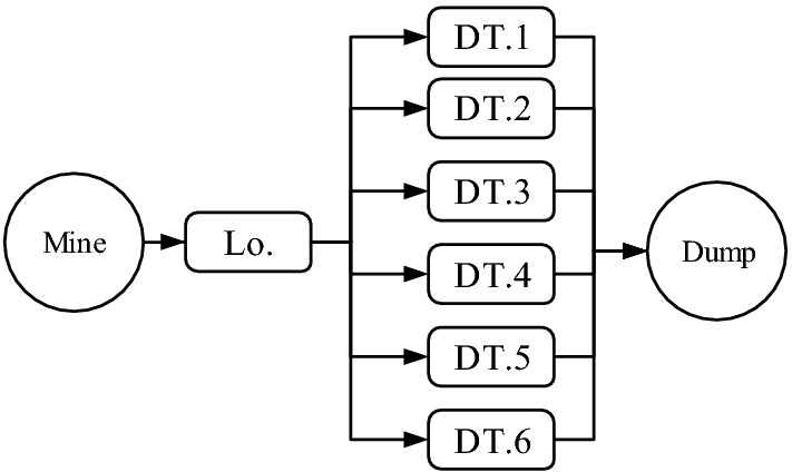
Block diagram of Sungun Copper mine’s transportation system

Results and discussion

In this section, the results of the covariate-based RMS and resilience estimations of the mine’s transportation system are presented, respectively.

RMS of the transportation system

In the first step, a database was established about the loader and dump-trucks subsystems. The collected database belonged to the period of fifteen months. It was obtained by daily operation reports and periodical maintenance reports. This database has contained the time between failures (TBFs), time to repairs (TTRs), and time to deliveries (TTDs) data and their associated observed covariates. The identified observed covariates are introduced in Table 2.

Table 2.

Identified observed covariates that are associated with the failure and repair database

Failure database						Repair database
Sub-system	Identified covariates		Sub-system	Identified covariates		Sub-system	Identified covariates
Wheel loader	v1	Shift	Dump-truck	v1'	Shift	Loader & Dump-truck	z1	Shift
	v2	Working place		v2'	Number of service		z2	Involved maintenance crew
	v3	Proportion with truck		v3'	Proportion with loader		z3	Weather condition
	v4	Weather condition		v4'	Rock fragmentation		z4	Precipitate
	v5	Precipitate		v5'	Slope of road		z5	Temperature
	v6	Temperature		v6'	Weather condition
	v7	Road condition		v7'	Precipitate
	v8	Number of service		v8'	Temperature
	v9	Rock fragmentation		v9'	Road condition
	v10	Rock kind		v10'	Rock kind
				v11'	Hauling distance

In Sungun copper mine, loader and dump-trucks have the same repair workstation. Hence, the identified observed covariates about the repair database are similar for each subsystem. Also, there were no observed covariates for the logistic database. The collected data were classified and sorted according to the identified covariates. The details of the identified covariates are presented in Appendix (see Table 8). In the second step, the time dependency of the identified observed covariates was checked by Schoenfeld residuals test. According to the results, some of the covariates that are related to the DT.1 subsystem have P-values less than 0.05. Hence, the effect of these covariates on the failure of this subsystem is time-dependent. Therefore, based on the experience and statistical approach, the failure database of DT.1 was stratified into three layers in a way that in each layer all covariates be time-independent. The results of Schoenfeld residuals test are shown in Appendix (see Tables 9 and 10).

Table 8.

Identified covariates for failure and repair database

Database	Subsystem	Identified covariates		Category (Score)
Failure database	Lo	v1	Shift	Morning (0)	Afternoon (1)	Night (2)
		v2	Working place	Dump (0)	Mining face (1)
		v3	Proportion with truck	Suitable (0)	Partly suitable (1)	Unsuitable (2)
		v4	Weather condition	Sunny (1)	Semi cloudy (2)	Cloudy (3)	Dense fog (4)
		v5	Precipitate	Continuous covariate
		v6	Temperature	Continuous covariate
		v7	Road condition	Normal (0)	Abnormal (1)
		v8	Number of service	Good (1)	Moderate (2)	Bad (3)
		v9	Rock fragmentation	Ore, dump (0)	Middle-Monzonite (1)	North-Monzonite (2)	Trachyte (3)	South-Monzonite (4)
		v10	Rock kind	Ore (0)		Monzonite (1)	Trachyte (2)
	DTs	v1′	Shift	Morning (0)	Afternoon (1)	Night (2)
		v2′	Number of service	Good (1)	Moderate (2)	Bad (3)
		v3′	Proportion with loader	Suitable (0)	Partly suitable (1)	Unsuitable (2)
		v4′	Rock fragmentation	Ore, oxide, dump (0)	Middle-Monzonite (1)	North-Monzonite (2)	Trachyte (3)	South-Monzonite (4)
		v5′	Slope of road	Same level (0)	Down (1)	Up (2)
		v6′	Weather condition	Sunny (1)	Semi cloudy (2)	Cloudy (3)	Dense fog (4)
		v7′	Precipitate	Continuous covariate
		v8′	Temperature	Continuous covariate
		v9′	Road condition	Normal (0)	Abnormal (1)
		v10′	Rock kind	Ore (0)		Monzonite (1)	Trachyte (2)
		v11′	Hauling distance	Short (0)	Normal (1)	Long (2)
	Lo. and DTs	z1	Shift	Morning (0)	Afternoon (1)	Night (2)
Repair database		z2	Involved maintenance crew	One (0)	More than one (1)
		z3	Weather condition	Sunny (1)	Semi cloudy (2)	Cloudy (3)	Dense fog (4)
		z4	Precipitate	Continuous covariate
		z5	Temperature	Continuous covariate

Table 9.

Proportionality assumption results for the loader and dump-trucks covariates based on the repair database

Covariate	P-value
	Lo	DT.1	DT.2	DT.3	DT.4	DT.5	DT.6
z1	0.965	0.812	0.556	0.991	0.919	0.947	0.858
z2	0.868	0.995	0.253	0.908	0.956	0.940	0.894
z3	0.865	0.944	0.781	0.984	0.755	0.842	0.982
z4	0.904	0.894	0.730	0.940	0.850	0.760	0.915
z5	0.376	0.677	0.914	0.735	0.909	0.428	0.777

Table 10.

Proportionality assumption results for the loader and dump-trucks covariates based on the failure database

Covariate	P-value	Covariate	P-value
	Lo		DT.1	DT.2	DT.3	DT.4	DT.5	DT.6
v1	0.99	v1′	0.513	0.624	0.989	0.979	0.695	0.945
v2	0.123	v2′	0.008	0.548	0.326	0.452	0.370	0.550
v3	0.527	v3′	0.001	0.448	0.896	0.814	0.695	0.972
v4	0.667	v4′	0.027	0.380	0.747	0.481	0.95	0.661
v5	0.364	v5′	0.534	0.294	0.748	0.826	0.529	0.738
v6	0.278	v6′	0.284	0.401	0.711	0.884	0.858	0.556
v7	0.893	v7′	0.520	0.495	0.473	0.477	0.893	0.311
v8	0.708	v8′	0.680	0.328	0.751	0.626	0.094	0.924
v9	0.879	v9′	0.170	0.710	0.608	0.775	0.637	0.880
v10	0.973	v10′	0.079	0.309	0.602	0.616	0.473	0.412
		v11′	0.861	0.906	0.843	0.822	0.931	0.920

In the third step, the unobserved heterogeneity among the collected databases was checked. The results of the heterogeneity tests for the failure, repair, and logistic databases are introduced in Appendix (see Table 11) Based on the results, failure data of Lo and DT.1 subsystems, repair data of Lo and all dump-trucks subsystems, and also logistic data of Lo and all dump-trucks subsystems have unobserved heterogeneities. It must be mentioned that the logistic data are the same for all dump-trucks subsystems due to the same inventory, spare parts, and repairs.

Table 11.

Likelihood ratio test results

Failure database			Repair database			Logistic database
Subsystem	R	P-value	Subsystem	R	P-value	Subsystem	R	P-value
Lo	14.930	0.000	Lo	15.540	0.000	Lo	10.440	0.000
DT.1 (1st layer)	0.210	0.332	DT.1	54.900	0.000	DT.s	2.880	0.045
DT.1 (2nd layer)	0.000	0.500	DT.2	17.710	0.000
DT.1 (3rd layer)	10.750	0.001	DT.3	70.310	0.000
DT.2	1.660	0.099	DT.4	52.610	0.000
DT.3	0.000	1.000	DT.5	26.950	0.000
DT.4	0.470	0.246	DT.6	65.280	0.000
DT.5	1.950	0.081
DT.6	2.040	0.077

In the fourth step, the suitable models were selected for the hazard, repair, and delivery rates of the subsystems. Firstly, based on the validation of the iid assumption using the trend and serial correlation tests for the failure, repair, and logistic data of the subsystems, the best models for the baseline hazard, repair, and delivery rates were selected (see Tables 5, 6, and 7). Secondly, based on the time dependency and heterogeneity tests, the suitable models for the hazard, repair, and delivery rates of the subsystems were selected. The results are introduced in Table 3. It must be mentioned, because the same inventory, spare parts, and repairs, all dump-trucks subsystems have the same delivery rate models. Afterward, the regression coefficients of the observed covariates, as well as the variance of Gamma distributions for each subsystem (i.e.,$\theta$) that have unobserved heterogeneity, were estimated. The results of the regression coefficients significance checking are introduced in Appendix (see Table 12). The observed covariates, which their regression coefficients P-values were greater than 0.05, have been excluded from the RMS estimation process. Furthermore, values of $\theta$ for each subsystem are introduced in Table 4. At the last step, based on the selected models, RMS functions were obtained for each subsystem. The results are introduced in Tables 5, 6, and 7. Finally, RMS estimation was carried out for 6.3 h of system operation (the considered time step is 0.7 h) using RMS functions. The results are illustrated in Figs 3, 4, and 5.

Table 5.

Obtained reliability functions for each subsystems

Subsystem	Baseline hazard rate parameters (PLP model*)		Reliability function
	b (Scale)	a (Shape)
Lo	9.592	1.950	$R_{Lo{.}_{\theta }}\left(t,\nu \right)={\left[1-0.97ln\left({\left(exp\left(-{\left(\frac{t}{9.592}\right)}^{1.95}\right)\right)}^{exp\left(-0.6{\nu }_1-1.05{\nu }_2+0.49{\nu }_4-0.17{\nu }_5-0.83{\nu }_{10}\right)}\right)\right]}^{\raisebox{1ex}{$-1$}\!\left/ \!\raisebox{-1ex}{$0.97$}\right.}$
DT.1 (1st layer)	7.123	1.293	$R_{\text{DT}.1}\left(t,{\nu }^{\prime }\right)={\left(\text{exp}\left(-{\left(\frac{t}{7.123}\right)}^{1.293}\right)\right)}^{exp\left(-2.02{\nu }_2^{{}^{\prime }}-1.04{\nu }_6^{{}^{\prime }}\right)}$
DT.1 (2nd layer)	7.319	1.611	$R_{\text{DT}.1}\left(t,{\nu }^{\prime }\right)={\left(\text{exp}\left(-{\left(\frac{t}{7.319}\right)}^{1.611}\right)\right)}^{exp\left(-1.94{\nu }_1^{{}^{\prime }}-0.6{\nu }_2^{{}^{\prime }}+0.58{\nu }_5^{{}^{\prime }}+0.7{\nu }_9^{{}^{\prime }}\right)}$
DT.1 (3rd layer)	24.600	2.339	$R_{\text{DT}.1{}_{\theta }}\left(t,{\nu }^{\prime }\right)={\left[1-2.040ln\left({\left(exp\left(-{\left(\frac{t}{24.6}\right)}^{2.339}\right)\right)}^{exp\left(-1.22{\nu }_2^{{}^{\prime }}+2.14{\nu }_5^{{}^{\prime }}+1.44{\nu }_6^{{}^{\prime }}\right)}\right)\right]}^{\raisebox{1ex}{$-1$}\!\left/ \!\raisebox{-1ex}{$2.040$}\right.}$
DT.2	22.271	0.969	$R_{\text{DT}.2}\left(t,{\nu }^{\prime }\right)={\left(\text{exp}\left(-{\left(\frac{t}{22.271}\right)}^{0.969}\right)\right)}^{exp\left(-0.64{\nu }_1^{{}^{\prime }}-0.68{\nu }_2^{{}^{\prime }}+0.65{\nu }_5^{{}^{\prime }}+0.26{\nu }_6^{{}^{\prime }}\right)}$
DT.3	44.742	1.012	$R_{\text{DT}.3}\left(t,{\nu }^{\prime }\right)={\left(\text{exp}\left(-{\left(\frac{t}{44.742}\right)}^{1.012}\right)\right)}^{exp\left(-0.44{\nu }_1^{{}^{\prime }}-0.82{\nu }_2^{{}^{\prime }}+0.28{\nu }_4^{{}^{\prime }}+0.87{\nu }_5^{{}^{\prime }}\right)}$
DT.4	14.549	1.301	$R_{\text{DT}.4}\left(t,{\nu }^{\prime }\right)={\left(\text{exp}\left(-{\left(\frac{t}{14.549}\right)}^{1.301}\right)\right)}^{exp\left(-1.08{\nu }_1^{{}^{\prime }}-0.98{\nu }_2^{{}^{\prime }}+0.29{\nu }_4^{{}^{\prime }}+0.66{\nu }_5^{{}^{\prime }}\right)}$
DT.5	30.569	0.988	$R_{\text{DT}.5}\left(t,{\nu }^{\prime }\right)={\left(\text{exp}\left(-{\left(\frac{t}{30.569}\right)}^{0.988}\right)\right)}^{exp\left(-0.6{\nu }_1^{{}^{\prime }}-0.65{\nu }_2^{{}^{\prime }}+0.35{\nu }_4^{{}^{\prime }}+0.45{\nu }_5^{{}^{\prime }}\right)}$
DT.6	28.420	1.012	$R_{\text{DT}.6}\left(t,{\nu }^{\prime }\right)={\left(\text{exp}\left(-{\left(\frac{t}{28.420}\right)}^{1.012}\right)\right)}^{exp\left(-0.68{\nu }_1^{{}^{\prime }}-0.57{\nu }_2^{{}^{\prime }}+0.82{\nu }_5^{{}^{\prime }}\right)}$

*PLP model: $\frac{a}{b}{\left(\frac{t}{b}\right)}^{a-1}$

Table 6.

Obtained maintainability functions for each subsystems

Subsystem	Baseline repair rate model’s parameters (PLP model)		Maintainability function
	b (Scale)	a (Shape)
Lo	2.474	1.348	$M_{Lo{.}_{\theta }}\left(t,z\right)=1-{\left[1-0.57ln\left({\left(exp\left(-{\left(\frac{t}{2.474}\right)}^{1.348}\right)\right)}^{exp\left(-2.35z_2-0.48c_3\right)}\right)\right]}^{\raisebox{1ex}{$-1$}\!\left/ \!\raisebox{-1ex}{$0.57$}\right.}$
DT.1	1.370	3.680	$M_{\text{DT}.1_{\theta }}\left(t,z\right)=1-{\left[1-3.22ln\left({\left(exp\left(-{\left(\frac{t}{1.37}\right)}^{3.68}\right)\right)}^{exp\left(-7.37z_2\right)}\right)\right]}^{\raisebox{1ex}{$-1$}\!\left/ \!\raisebox{-1ex}{$3.22$}\right.}$
DT.2	1.486	2.211	$M_{\text{DT}.2_{\theta }}\left(t,z\right)=1-{\left[1-0.86ln\left({\left(exp\left(-{\left(\frac{t}{1.486}\right)}^{2.211}\right)\right)}^{exp\left(-3.01z_2\right)}\right)\right]}^{\raisebox{1ex}{$-1$}\!\left/ \!\raisebox{-1ex}{$0.86$}\right.}$
DT.3	1.239	3.547	$M_{\text{DT}.3_{\theta }}\left(t,z\right)=1-{\left[1-3.43ln\left({\left(exp\left(-{\left(\frac{t}{1.239}\right)}^{3.547}\right)\right)}^{exp\left(-7.51z_2\right)}\right)\right]}^{\raisebox{1ex}{$-1$}\!\left/ \!\raisebox{-1ex}{$3.43$}\right.}$
DT.4	1.710	2.103	$M_{\text{DT}.4_{\theta }}\left(t,z\right)=1-{\left[1-1.1ln\left({\left(exp\left(-{\left(\frac{t}{1.71}\right)}^{2.103}\right)\right)}^{exp\left(-0.55z_1-2.92z_2\right)}\right)\right]}^{\raisebox{1ex}{$-1$}\!\left/ \!\raisebox{-1ex}{$1.11$}\right.}$
DT.5	1.056	3.493	$M_{\text{DT}.5_{\theta }}\left(t,z\right)=1-{\left[1-3.3ln\left({\left(exp\left(-{\left(\frac{t}{1.056}\right)}^{3.493}\right)\right)}^{exp\left(-7.26z_2-0.67z_3\right)}\right)\right]}^{\raisebox{1ex}{$-1$}\!\left/ \!\raisebox{-1ex}{$3.3$}\right.}$
DT.6	1.394	3.453	$M_{\text{DT}.6_{\theta }}\left(t,z\right)=1-{\left[1-2.86ln\left({\left(exp\left(-{\left(\frac{t}{1.394}\right)}^{3.453}\right)\right)}^{exp\left(-6.7z_2\right)}\right)\right]}^{\raisebox{1ex}{$-1$}\!\left/ \!\raisebox{-1ex}{$2.86$}\right.}$

Table 7.

Obtained supportability functions for each subsystems

Subsystem	Baseline delivery rate model’s parameters (PLP model)		Supportability function
	b (Scale)	a (Shape)
Lo	0.318	1.397	$S_{Lo{.}_{\theta }}\left(t\right)=1-{\left[1-0.588ln\left(exp\left(-{\left(\frac{t}{0.318}\right)}^{1.397}\right)\right)\right]}^{\raisebox{1ex}{$-1$}\!\left/ \!\raisebox{-1ex}{$0.588$}\right.}$
DTs	8.900	1.245	$S_{\text{DTs}{.}_{\theta }}\left(t\right)=1-{\left[1-1.050ln\left(exp\left(-{\left(\frac{t}{8.9}\right)}^{1.245}\right)\right)\right]}^{\raisebox{1ex}{$-1$}\!\left/ \!\raisebox{-1ex}{$1.050$}\right.}$

Table 3.

The results of the hazard, repair, and delivery models selection

Failure database		Repair database		Logistic database
Subsystem	Model	Subsystem	Model	Subsystem	Model
Lo	Mixed Cox model	Lo	Mixed Cox model	Lo	Mixed Cox model
DT.1 (1st layer)	Cox model	DT.1	Mixed Cox model	DT.s	Mixed Cox model
DT.1 (2nd layer)	Cox model	DT.2	Mixed Cox model
DT.1 (3rd layer)	Mixed Cox model	DT.3	Mixed Cox model
DT.2	Cox model	DT.4	Mixed Cox model
DT.3	Cox model	DT.5	Mixed Cox model
DT.4	Cox model	DT.6	Mixed Cox model
DT.5	Cox model
DT.6	Cox model

Table 12.

Results of the coefficients significance checking

Covariates	P-value	Covariates	P-value
	Lo		DT.1 (3rd layer)	DT.2	DT.3	DT.4	DT.5	DT.6
Failure database
v1	0.02	v1′	0.07	0.04	0.04	0.00	0.01	0.00
v2	0.00	v2′	0.03	0.00	0.00	0.00	0.00	0.00
v3	0.53	v3′	-	0.65	0.95	0.23	0.21	0.82
v4	0.00	v4′	0.33	0.54	0.00	0.00	0.00	0.93
v5	0.01	v5′	0.00	0.00	0.00	0.00	0.00	0.00
v6	0.06	v6′	0.02	0.02	0.35	0.28	0.50	0.97
v7	0.37	v7′	0.09	0.77	0.95	0.06	0.57	0.81
v8	0.52	v8′	0.40	0.59	0.40	0.07	0.13	0.66
v9	0.18	v9′	0.52	0.03	0.24	0.08	0.02	0.08
v10	0.03	v10′	0.81	0.14	0.19	0.05	0.01	0.17
		v11′	0.07	0.09	0.06	0.21	0.00	0.00
Repair database
z1	0.39	z1	0.13	0.18	0.56	0.01	0.66	0.30
z2	0.00	z2	0.00	0.00	0.00	0.00	0.00	0.00
z3	0.00	z3	0.79	0.15	0.53	0.19	0.01	0.90
z4	0.54	z4	0.91	0.31	0.96	0.27	0.59	0.95
z5	0.48	z5	0.98	0.72	0.85	0.05	0.61	0.78

Table 4.

The values of the variance $\theta$

Failure database		Repair database		Logistic database
Subsystem	$\theta$	Subsystem	$\theta$	Subsystem	$\theta$
Lo	0.970	Lo	0.570	Lo	0.588
DT.1 (3rd layer)	2.040	DT.1	3.220	DTs	1.050
DT.2	–	DT.2	0.860
DT.3	–	DT.3	3.430
DT.4	–	DT.4	1.110
DT.5	–	DT.5	3.300
DT.6	–	DT.6	2.860

Fig. 3.

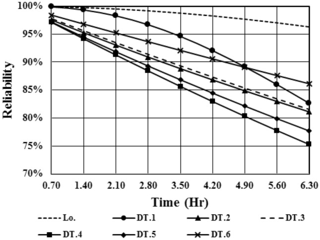
Subsystems reliability estimation results

Fig. 4.

Subsystems maintainability estimation results

Fig. 5.

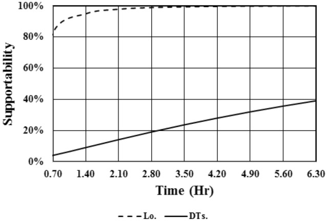
Subsystems supportability estimation results

Based on Fig. 3, at a certain time, the reliability of the loader subsystem will be more than dump-truck subsystems. For example, 2.80 h after starting the subsystems activity, the reliability of loader and DT.4 will be equal to 0.992 and 0.884, respectively. It means after the 2.8 h of subsystems operation, the probability of DT.4 failure will be 0.36% more than loader failure probability. This value for 6.30 h after starting the activity will be increased to 21.02%. According to Fig. 4, the maintainability of DT.2 will be higher than the loader subsystem maintainability. After the 2.8 h of activity, the repair probability of DT.2 will be 53.1% more than the loader repair probability. Other dump-truck subsystems have approximately the same maintainability, which means their repair probabilities are the same as each other. Figure 5 indicates that the loader subsystem will have better supporting (in the form of spare parts logistics, maintenance facilities, workforce, etc.) than dump-truck subsystems. Concerning the results, the probability of supporting the dump-truck subsystems after 6.3 h of system operation will be less than 40%, which means these subsystems will have a great potential to suspend the transportation system operation in the face of failure events.

Resilience of the transportation system

According to Fig. 2, the ore transportation system is a series–parallel system. It must be mentioned the values of the PHM system efficiency and organizational resilience were considered as the constant values in this work (${\beta }_3=0.85$ and ${\beta }_4=0.75$) (Rød et al. 2016). Finally, using the obtained results, the resilience of the ore transportation subsystems for 6.3 h of operation were analyzed (see Fig. 6).

Fig. 6.

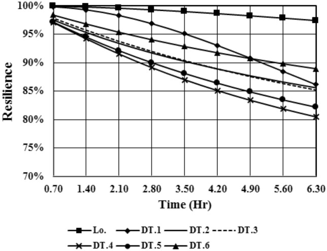
Transportation system’s subsystems resilience analysis results for 6.30 h of activity

As can be seen, the loader subsystem has higher resilience than other subsystems. Whereas, dump-truck subsystems will have lower resilience than the loader subsystem. For example, 6.30 h after starting the activity, the resilience of DT.6 will be reached to 86.92%. Therefore, in the face of disruptions or failures, the loader subsystem will have a more probability to be resilience against the failures.

Ultimately, the resilience of the system for 6.30 h of activity is shown in Fig. 7. As can be seen, the resilience of the ore transportation system will be equal to 97.43% after 6.30 h of activity. In other words, the system will have a 97.43% probability to withstand against and to recover its normal function in the case of disruption. However, maintaining or enhancing this ability is one of the most critical issues for Sungun copper mine management.

Fig. 7.

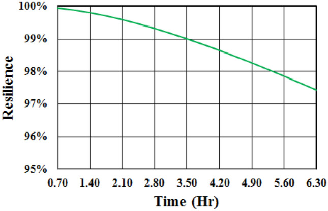
The results of the transportation system resilience analysis for 6.30 h of activity

Generally, to increase or maintain the resilience of the system, the mine management should be more focused on the subsystems with low RMS. Improvement of the preventive maintenance activates or increasing redundancy in dump-truck and loader subsystems like adding the new dump-trucks or loaders to the ore transportation system are some ways to increment the reliability of the ore transportation system. Maintainability of loader subsystems can be increased by the improvement of repair facilities and using skilled workers etc. Moreover, the supportability of dump-truck subsystems can be increased using suitable spare parts logistics, using fast and secure coordination of the demand for spare parts and enhancing spare parts transportation speed to the workstation, etc.

Conclusion

Previously large scale disruptive events have shown that risk management is not enough to protect systems and infrastructures against disruptive events. Furthermore, anticipating the characteristics of all types of disruption, such as occurrence probability and level of consequences, is impossible. Thus, in the last years, systems’ managers have shifted their focus from building a robust system by risk management to establish a resilient system using resilience management. Robust systems experience sudden failure in case of disruption, while resilient systems absorb the adverse impacts, adapt to and recover their desired performance level after a disruption. Resilience analysis is the first step to build a resilient system. Frequently, resilience of systems is analyzed only using historical data. However, to have a precise resilience analysis, the effect of risk factors (observed and unobserved covariates) should be considered. Thus, in this research, a formulation was introduced to model risk factors on complex system resilience. Ultimately, to demonstrate how it can be used in a real case, it was applied for a mine’s transportation system. According to the results, if there is a failure or disruption in the transportation system, it will have a 97.43% probability to be resilient against the failure events. It should be noted the observed and unobserved covariates may have a significant effect on the system resilience. Hence, it is important to identify these covariates. Generally, to increase or maintain the resilience of the mine’s transportation system, the mine’s management should be more focused on the subsystems with low reliability, maintainability, and supportability. The application of the resilience concept in the field of the mining industry will be useful for mining companies and service providers that use a variety of engineering systems for continuous production. This concept will help them to minimize the downtime of mine’s production systems and keep the costs down.

Appendix

See Tables 8, 9, 10, 11, and 12.

References

- Amico AD, Currà E. The role of urban built heritage in qualify and quantify resilience. Specific issues in Mediterranean City. Procedia Econ Finance. 2014;18:181–189. doi: 10.1016/S2212-5671(14)00929-0. [DOI] [Google Scholar]
- Barabadi A. Reliability and spare parts provision considering operational environment: a case study. Int J Perform Eng. 2012;8:497–506. [Google Scholar]
- Barabadi A, Barabady J, Markeset T. Maintainability analysis considering time-dependent and time-independent covariates. Reliab Eng Syst Saf. 2011;96:210–217. doi: 10.1016/j.ress.2010.08.007. [DOI] [Google Scholar]
- Barabadi A, Ghiasi MH, Nouri Qarahasanlou A, Mottahedi A. A holistic view of health infrastructure resilience before and after COVID-19. ABJS. 2020;8:262. doi: 10.22038/abjs.2020.47817.2360. [DOI] [PMC free article] [PubMed] [Google Scholar]
- Barabadi A, Markeset T. Reliability and maintainability performance under Arctic conditions. Int J Syst Assur Eng Manag. 2011;2:205–217. doi: 10.1007/s13198-011-0071-8. [DOI] [Google Scholar]
- Barabadi Reza, Ataei Mohammad, Khalokakaie Reza, Nouri Qarahasanlou Ali. Spare-part management in a heterogeneous environment. PLOS ONE. 2021;16(3):e0247650. doi: 10.1371/journal.pone.0247650. [DOI] [PMC free article] [PubMed] [Google Scholar]
- Brown ED, Williams BK. Resilience and resource management. Environ Manag. 2015;56:1416–1427. doi: 10.1007/s00267-015-0582-1. [DOI] [PMC free article] [PubMed] [Google Scholar]
- Cook A, Delgado L, Tanner G, Cristóbal S. Measuring the cost of resilience. J Air Transp Manag. 2016;56:38–47. doi: 10.1016/j.jairtraman.2016.02.007. [DOI] [Google Scholar]
- Finkelstein M. Imperfect repair and lifesaving in heterogeneous populations. Reliab Eng Syst Saf. 2007;92:1671–1676. doi: 10.1016/j.ress.2006.09.018. [DOI] [Google Scholar]
- Garmabaki AHS, Ahmadi A, Block J, Pham H, Kumar U. A reliability decision framework for multiple repairable units. Reliab Eng Syst Saf. 2016;150:78–88. doi: 10.1016/j.ress.2016.01.020. [DOI] [Google Scholar]
- Ghomghaleh Awat, Khaloukakaie Reza, Ataei Mohammad, Barabadi Abbas, Nouri Qarahasanlou Ali, Rahmani Omeid, Beiranvand Pour Amin, Dragan Dejan. Prediction of remaining useful life (RUL) of Komatsu excavator under reliability analysis in the Weibull-frailty model. PLOS ONE. 2020;15(7):e0236128. doi: 10.1371/journal.pone.0236128. [DOI] [PMC free article] [PubMed] [Google Scholar]
- Gutierrez RG (2002) Parametric frailty and shared frailty survival models. Stand Genomic Sci 2:22–44. 10.1177/1536867X0200200102
- Holling CS. Resilience and stability of ecological systems. Annu Rev Ecol Syst. 1973;4:1–23. doi: 10.1146/annurev.es.04.110173.000245. [DOI] [Google Scholar]
- Kleinbaum DG, Klein M. Evaluating the proportional hazards assumption survival analysis. Statistics for biology and health. New York, NY: Springer; 2012. [Google Scholar]
- Kumar D, Klefsjo B. Proportional hazards model: a review. Reliab Eng Syst Saf. 1994;44:177–188. doi: 10.1016/0951-8320(94)90010-8. [DOI] [Google Scholar]
- Lancaster T. Econometric methods for the duration of unemployment. Econometrica. 1979;47:939. doi: 10.2307/1914140. [DOI] [Google Scholar]
- Meng F, Fu G, Farmani R, Sweetapple C, Butler D. Topological attributes of network resilience: a study in water distribution systems. Water Res. 2018;143:376–386. doi: 10.1016/j.watres.2018.06.048. [DOI] [PubMed] [Google Scholar]
- Mottahedi Adel, Sereshki Farhang, Ataei Mohammad, Nouri Qarahasanlou Ali, Barabadi Abbas. The Resilience of Critical Infrastructure Systems: A Systematic Literature Review. Energies. 2021;14(6):1571. doi: 10.3390/en14061571. [DOI] [Google Scholar]
- Müller F, Bergmann M, Dannowski R, Dippner JW, Gnauck A, Haase P, Jochimsen MC, Kasprzak P, Kröncke I, Kümmerlin R, Küster M, Lischeid G, Meesenburg H, Merz C, Millat G, Müller J, Padisák J, Schimming CG, Schubert H, Schult M, Selmeczy G, Shatwell T, Stoll S, Schwabe M, Soltwedel T, Straile D, Theuerkauf M. Assessing resilience in long-term ecological data sets. Ecol Ind. 2016;65:10–43. doi: 10.1016/j.ecolind.2015.10.066. [DOI] [Google Scholar]
- Najarian M, Lim GJ. Design and assessment methodology for system resilience metrics. Risk Anal. 2019 doi: 10.1111/risa.13274. [DOI] [PubMed] [Google Scholar]
- National Infrastructure Advisory Council . Critical infrastructure resilience: final report and recommendations. US: National Infrastructure Advisory Council, Department of Homeland Security; 2009. [Google Scholar]
- Omer M, Mostashari A, Lindemann U. Resilience analysis of soft infrastructure systems. Procedia Comput Sci. 2014;28:873–882. doi: 10.1016/j.procs.2014.03.104. [DOI] [Google Scholar]
- Pant R, Barker K, Zobel CW. Static and dynamic metrics of economic resilience for interdependent infrastructure and industry sectors. Reliab Eng Syst Saf. 2014;125:92–102. doi: 10.1016/j.ress.2013.09.007. [DOI] [Google Scholar]
- Petersen L, Lundin E, Fallou L, Sjöström J, Lange D, Teixeira R, Bonavita A. Resilience for whom? The general public’s tolerance levels as CI resilience criteria. Int J Crit Infrastruct Prot. 2020;28:100340. doi: 10.1016/j.ijcip.2020.100340. [DOI] [Google Scholar]
- Qarahasanlou AN, Barabadi A, Ayele YZ. Production performance analysis during operation phase: a case study. Proc Inst Mech Eng Part O J Risk Reliab. 2018;232:559–575. doi: 10.1177/1748006X17744383. [DOI] [Google Scholar]
- Rehak D. Assessing and strengthening organisational resilience in a critical infrastructure system: case study of the Slovak Republic. Saf Sci. 2020;123:104573. doi: 10.1016/j.ssci.2019.104573. [DOI] [Google Scholar]
- Rød B, Barabadi A, Gudmestad OT (2016) Characteristics of arctic infrastructure resilience: application of expert judgement. Presented at the 26th international ocean and polar engineering conference, 26 June-2 July, International Society of Offshore and Polar Engineers, Rhodes, Greece
- Rod Bjarte, Barabadi Abbas, Naseri Masoud. Recoverability Modeling of Power Distribution Systems Using Accelerated Life Models: Case of Power Cut due to Extreme Weather Events in Norway. Journal of Management in Engineering. 2020;36(5):05020012. doi: 10.1061/(ASCE)ME.1943-5479.0000823. [DOI] [Google Scholar]
- Vugrin ED, Warren DE, Ehlen MA. A Resilience assessment framework for infrastructure and economic systems: quantitative and qualitative resilience analysis of petrochemical supply chains to a Hurricane. Process Saf Prog. 2011;30:280–290. doi: 10.1002/prs.10437. [DOI] [Google Scholar]
- Walker B, Nilakant V, Baird R (2014) Promoting organisational resilience through sustaining engagement in a disruptive environment: what are the implications for HRM? Human Resources Institute of New Zealand Research Forum
- Youn BD, Hu C, Wang PF. Resilience-driven system design of complex engineered systems. J Mech Des. 2011;133:1–15. doi: 10.1115/1.4004981. [DOI] [Google Scholar]
- Zaki Rezgar, Barabadi Abbas, Qarahasanlou Ali Nouri, Garmabaki A. H. S. A mixture frailty model for maintainability analysis of mechanical components: a case study. International Journal of System Assurance Engineering and Management. 2019;10(6):1646–1653. doi: 10.1007/s13198-019-00917-3. [DOI] [Google Scholar]
- Zhang N, Huang H. Resilience analysis of countries under disasters based on multisource data: resilience analysis of countries under disasters. Risk Anal. 2018;38:31–42. doi: 10.1111/risa.12807. [DOI] [PubMed] [Google Scholar]