An automatic EEG-based sleep staging system with introducing NAoSP and NAoGP as new metrics for sleep staging systems

Abstract

Different biological signals are recorded in sleep labs during sleep for the diagnosis and treatment of human sleep problems. Classification of sleep stages with electroencephalography (EEG) is preferred to other biological signals due to its advantages such as providing clinical information, cost-effectiveness, comfort, and ease of use. The evaluation of EEG signals taken during sleep by clinicians is a tiring, time-consuming, and error-prone method. Therefore, it is clinically mandatory to determine sleep stages by using software-supported systems. Like all classification problems, the accuracy rate is used to compare the performance of studies in this domain, but this metric can be accurate when the number of observations is equal in classes. However, since there is not an equal number of observations in sleep stages, this metric is insufficient in the evaluation of such systems. For this purpose, in recent years, Cohen’s kappa coefficient and even the sensitivity of NREM1 have been used for comparing the performance of these systems. Still, none of them examine the system from all dimensions. Therefore, in this study, two new metrics based on the polygon area metric, called the normalized area of sensitivity polygon and normalized area of the general polygon, are proposed for the performance evaluation of sleep staging systems. In addition, a new sleep staging system is introduced using the applications offered by the MATLAB program. The existing systems discussed in the literature were examined with the proposed metrics, and the best systems were compared with the proposed sleep staging system. According to the results, the proposed system excels in comparison with the most advanced machine learning methods. The single-channel method introduced based on the proposed metrics can be used for robust and reliable sleep stage classification from all dimensions required for real-time applications.

Electronic supplementary material

The online version of this article (10.1007/s11571-020-09641-2) contains supplementary material, which is available to authorized users.

Introduction

The classification of sleep stages is very important both in the diagnosis and treatment of sleep problems and in research, such as child behavior analysis. Experts in this field divide biological signals such as EEG, electromyography (EMG), and electrooculography (EOG) into 30-s slices (epochs) and then examine the slices one by one for determining the sleep stages. The large number of biological signal recordings may cause poor-quality signal recording due to the comfort restrictions it will impose on the patient (Zhu et al. 2014). For this, the use of EEG and, more importantly, a single EEG channel has many advantages such as low cost, patient comfort, ease of electrode placement, and low computational burden. Therefore, the classification of sleep stages with a single EEG channel has attracted the attention of numerous researchers.

According to the R&K standard (Rechtschaffen and Kales 1968), sleep is divided into two general stages: REM (rapid eye movement) and NonREM (no rapid eye movement). The NREM stage is divided into four sub-stages of NREM1, 2 (superficial sleep), 3, 4 (deep sleep). REM sleep is also called paradoxical sleep. In a healthy person, each of these stages takes 15–20 min, and a full cycle takes 75–90 min. After the completion of a cycle, stages NREM1 through REM are repeated again (Sharma et al. 2019a).

The NREM1 stage is the phase of transition from wakefulness to sleep and may take 1–5 min. At this stage, the amplitude of the EEG signal is small and it includes theta and alpha waves. During the NREM2 stage, sleep spiders and k-complexes appear in the EEG signal, which will have slightly lower frequencies than alpha waves. In the NREM3 stage, more than 20% and below 50% delta wave appear in every 30 s of epochs. The frequency of the delta wave is below 2 Hz and its amplitude is above 75 micro-volts. Night terror and sleepwalking are experienced in this stage (Sharma et al. 2019a). The NREM4 stage is similar to the NREM3 stage, but the delta wave constitutes more than 50% of each epoch of this stage. Upon waking up from this stage, a sense of disorientation is very common (Sharma et al. 2019a). The NREM3 and NREM4 stages are called deep sleep. The REM stage has an EEG signal with a small amplitude and mixed frequencies. At this stage, a rapid movement of the eyes appears and the EMG signal of the chin muscles is very small. Vertex signals are rare in this evolution but sawtooth waves can be observed. The EEG signal of the REM stage is similar to the EEG signal of the NREM1 and wake stages. The jaw's EMG signal is used to distinguish REM and NREM1 stages (Shephard 1991). Wakefulness is generally divided into two stages. When awake, the EEG signal with eyes wide open has a low amplitude and a high frequency. In eyes-closed vigilance, the alpha wave appears predominantly in the EEG signal (Shephard 1991).

As previously mentioned, the common clinical method for classifying sleep stages is the visual evaluation by experts that constitutes looking directly at the EEG signals for comparing certain waveforms to previously known wave signals according to the R&K standard. The classification of signals in this way is very tiring and time-consuming and the margin of error is high (Boashash and Ouelha 2016; Akben and Alkan 2016). Moreover, the results of the visual evaluation techniques depend on the experience of the expert, and the accuracy rate is below 90% (Penzel and Conradt 2000). In addition, the slowness of this method poses serious problems for research in this domain (Hassan and Bhuiyan 2017, 2016), and some clinical treatments may require the patient's sleep stages to be examined very quickly (Hsu et al. 2013; Lajnef 2015). The software-supported classification of sleep stages will accelerate this process and significantly contribute to its accuracy (Li et al. 2016).

The literature presents numerous studies in sleep stage identification (Ronzhina et al. 2012; Liang et al. 2012), sleep disorder identification by using EEG (Dhok et al. 2020) and electrocardiogram (ECG) (Sharma et al. 2018b, 2019b). Ronzhina et al. classified sleep stages with an artificial neural network classifier using a single EEG channel by a method based on power spectral density (Ronzhina et al. 2012). In another study, features were extracted from the EEG signal using the Renyi entropy and the stages were classified (Liang et al. 2012). In Sharma et al. (2018a), a new single-channel EEG based sleep-stages identification system using a three-band time–frequency localized wavelet filter bank for feature extraction and support vector machine (SVM) for classification was developed. They tested the proposed method in a large dataset and achieved a 91.5% accuracy rate in a six-stage case. Moreover, Kayikcioglu et al. proposed a feature extraction and classification method based on the auto-regressive (AR) model and partial least squares (PLS) algorithm to classify the sleep and wake stages (Kayikcioglu et al. 2015).

The open-access PhysioNet (Goldberger et al. 2000) database is frequently utilized to compare the methods proposed for the classification of sleep stages. One of the most frequently used datasets in this database is the Sleep-EDF dataset (Kemp et al. 2000), where EDF stands for European Define Format. More information about this data set is given in the Materials and Method section. Not just the researchers using this data set, but all the sleep scoring researchers use the accuracy rate and Cohen’s kappa coefficient (Cohen 1960) to compare their proposed system with existing systems. Since the classification of the stage NREM1 is difficult compared to other stages, the sensitivity of this stage has been used in recent years as a comparison metric of sleep staging systems. The study, which obtained the highest accuracy rate on the Pz-Oz channel in the sleep-EDF dataset, was conducted by Ghimatgar et al. (2019). The authors reached a 94.55% accuracy rate. However, in the confusion matrix via leave-one-out cross-validation (LOO-CV) strategy obtained in this study, the sensitivity values of NREM1 were around 11%. In the testing phase, the sensitivity of NREM1 for the five-stage sleep classification case was given as 10.93%. In this study, sensitivities were not given for the six-stage sleep classification case. Moreover, in a study based on deep learning (Mousavi et al. 2019), the highest sensitivity was obtained for NREM1. This value was around 68%, although the accuracy rate obtained from the system's confusion matrix was around 90%. From among the studies conducted with the machine learning methods, the highest NREM1 sensitivity was 42.05% in the six-stage sleep classification case that was achieved by Hassan and Bhuiyan (2017). The accuracy rate of this study was specified as 88.07%.

Generally, several metrics are available to evaluate the performance of a classification phase, such as accuracy rate, sensitivity, specificity, Cohen’s kappa coefficient, and F-measure. As mentioned in sleep staging systems, accuracy rate, Cohen’s kappa coefficient, and NREM1 sensitivity are among the most widely used metrics. The superiority of one system over another is not acceptable only by using these metrics. The reason is that a system may be successful in one metric, while it may not be successful in another metric or metrics. The study by Ghimatgar et al. (2019) is an example of this. In this study, although the accuracy rate was specified as 95.40% in the five-stage sleep classification case, the NREM1 sensitivity was calculated as 10.93%. In Hassan and Bhuiyan (2017), the accuracy rate was 88.07%, whereas the NREM1 sensitivity equaled 42.05%. In addition, systems often borrow from the sensitivity of other stages to increase certain stage sensitivity. This may not always be clear. Therefore, a new parameter is needed to evaluate sleep staging systems from all dimensions. In Aydemir (2020) a polygon area metric (PAM) consisting of those parameters, instead of six different parameters, was proposed for evaluating the classifier performance. Thus, the performance of a classifier can be easily evaluated with a single metric without the need to compare various metrics. The stability and validity of the proposed metric were tested on seven data sets with the k-nearest neighbor (k-NN), support vector machines (SVM), and linear discriminant analysis (LDA) classifiers.

In this paper, we propose two new metrics based on PAM for the evaluation of sleep staging systems. One of these two metrics evaluates the overall sensitivity of the system, and the other one evaluates the system from all dimensions. In this way, the sensitivity of the systems to all sleep stages can be measured with a single metric. Also, the superiority of the systems to each other can be expressed with only one metric. In addition, in this study, a new sleep staging system without writing codes was proposed with the two applications offered by MATLAB (2019b). Feature extraction, evaluation, and selection were performed by using Diagnostic Feature Designer and the classification by Classification Learner applications. The system in the proposed general metric is superior to the existing machine learning systems.

The rest of this article is organized as follows: “Materials and methods” section introduces the materials and method. Data acquisition, feature extraction, and classifications are also described in this section. “Results” section presents the results. Finally, in “Discussion” and “Conclusion” sections, the discussion and conclusions are respectively given.

Materials and methods

Data set

In order to perform a comparison between the proposed system and existing systems, the sleep-EDF dataset (Kemp et al. 2000) in the PhysioNet (Goldberger et al. 2000) database was employed in this study. This data set consists of eight Caucasian males and females aged 21–35 years. Four of them are healthy (as marked SC and recorded in 1989) and four of them with mild difficulty in falling asleep (as marked ST and recorded in 1994). The subjects did not use any medication. EEG recordings were obtained from the Fpz-Cz, and Pz-Oz channels with a sampling frequency of 100 Hz. Also, dataset is included horizontal EOG. According to R&K standards, the signals in this data set were divided into epochs of 30 s and classified into six sleep stages by a clinician. Each person's hypnogram data were provided next to the set. Table 1 shows the number of epochs obtained from eight individuals per stage. The columns named S1, S2, S3, S4, R, and W are NREM1, NREM2, NREM3, NREM4, REM, and wake, respectively. In addition, the number of training and test epochs appears in this table. Based on the studies that used this dataset, half of the epochs of each stage were allocated for training and a half for testing.

Table 1.

Epoch distributions of sleep stages in the sleep-EDF dataset (total, training, and testing set)

	S1	S2	S3	S4	R	W
Total	604	3621	672	627	1609	8031
Train	302	1810	336	313	804	4015
Test	302	1811	336	314	805	4016

In studies classifying sleep stages, five classification cases are generally taken into account (Table 2). In the six-stage sleep classification case, each of the six stages of sleep is considered as a separate class, while in the five-stage sleep classification case, NREM3 and NREM4 classes are combined to express a single class. By combining NREM1 and NREM2, a four-stage sleep classification case is obtained. If all NREM stages are considered in a single class, a three-stage sleep classification case emerges with REM and wake. Finally, in the two-stage sleep classification case, all sleep stages are classified against the wake stage.

Table 2.

Sleep stages classification cases

Classification cases	Sleep stages
6	S1	S2	S3	S4	R	W
5	S1	S2	S3 + S4		R	W
4	S1 + S2		S3 + S4		R	W
3	S1 + S2 + S3 + S4				R	W
2	S1 + S2 + S3 + S4 + R					W

Pre-processing

The Butterworth filter, which passes a band with a range of 0.1–45 Hz from the third order for 30-s epochs, was used. The MATLAB filtfilt command was used to reduce the phase shift to zero. Then, normalization was performed to increase the consistency of the EEG signal. For this purpose, the z-score normalization method was applied. The raw and processed version of a 30-s epoch belonging to the wake stage is displayed in Fig. 1. It can be seen that the amplitude of the processed signal is normalized, and the frequency components are in the filter band.

Fig. 1.

An example of the wake stage’s EEG epoch before and after pre-processing

Feature extraction and selection

As mentioned earlier, in this study, the feature extraction process was performed with the Diagnostic Feature Designer application of MATLAB software. This application uses a multi-functional graphical interface, which allows features to be obtained from the signal in both the time and the frequency domain and evaluates the effectiveness of the extracted features with histograms. This MATLAB application provides quick and easy feature extraction, selection, and testing, without the need to write codes. In addition, it evaluates the contribution of the features to accuracy performance with different metrics and ranks the features based on their importance.

In this study, 13 features for the time domain and 10 features for the frequency domain were extracted from each epoch. Features extracted from the time domain were standard deviation, root mean square (RMS), crest factor, impulse factor, clearance factor, signal-to-noise ratio (SNR), peak value, signal-to-noise and distortion ratio (SINAD), kurtosis, shape factor, skewness, mean, and total harmonic distortion (THD). The calculation of these features is given in Table 3. In this table, n denotes the number of samples (length of epoch), x signal, $\overline{x}$ average of signal, σ standard deviation, pv peak value, and H the harmonies of the fundamental frequency.

Table 3.

Time-domain extracted features by using the Diagnostic feature designer app

$Mean=\frac{1}{n}\sum _1^n{x}_i$	$Peakvalue=max\left|x_i\right|$
$RMS=\sqrt{\frac{1}{n}\sum _{i=1}^n{x}_i^2}$	$Impulsefactor=\frac{\mathit{pv}}{\frac{1}{n}{\sum }_1^n\left|x_i\right|}$
$Standarddeviation=\sqrt{\frac{1}{n}\sum _{i=1}^n{\left(x_i-\overline{x}\right)}^2}$	$Clearancefactor=\frac{\mathit{pv}}{{\left(\frac{1}{n}{\sum }_1^n\left|x_i\right|\right)}^2}$
$Skewness=\frac{{\sum }_{i=1}^n{\left(x_i-\overline{x}\right)}^3}{\left(n-1\right){\sigma }^3}$	$SNR=\frac{P_{\mathit{signal}}}{P_{\mathit{noise}}}$
$Kurtosis=\frac{{\sum }_{i=1}^n{\left(x_i-\overline{x}\right)}^4}{\left(n-1\right){\sigma }^4}$	$SINAD=\frac{P_{\mathit{signal}}+P_{\mathit{distortion}}+P_{\mathit{noise}}}{P_{\mathit{noise}}+P_{\mathit{distortion}}}$
$Shapefactor=\frac{\sqrt{\frac{1}{n}{\sum }_{i=1}^n{x}_i^2}}{\frac{1}{n}{\sum }_{i=1}^n\left|x_i\right|}$	$THD=\frac{\sqrt{H_2^2+H_3^2+H_4^2+H_5^2}}{H_1}$
$Crestfactor=\frac{\mathit{pv}}{\sqrt{\frac{1}{n}{\sum }_{i=1}^n{x}_i^2}}$

The Welch method was employed for the frequency domain. By choosing the Hanning window, the Welch method calculates the power spectrum of the signal in the frequency range of 0–45 Hz. Window lengths were adjusted as 100 samples and 75% overlap. Taking into account the frequency band ranges of the EEG signals, the average power frequency ranges were calculated (Table 4), and 10 features were obtained.

Table 4.

Frequency band ranges used in feature extraction

Order	Band	Frequency (Hz)
1	Theta 1	0.27–2.16
2	Theta 2	2.16–4.14
3	Delta 1	4.14–6.03
4	Delta 2	6.03–8.01
5	Alpha	8.01–12.06
6	Beta 1	12.06–20.07
7	Beta 2	20.07–29.97
8	Total	0.27–29.97
9	Theta	0.27–4.14
10	Delta	4.14–8.01

Also, by using the Diagnostic Feature Designer app. features obtained from the time and frequency domains were evaluated using the Kruskal–Wallis and analysis of variance (ANOVA) tests. Both methods listed features from the most significant to the least insignificant feature.

Classification

The second application used in this study was the Classification Learner app. This application enables the features to look interactive and allows for selecting the features, determining validation strategies, preferring the training algorithm, and evaluating its performance. The application includes supervised machine learning algorithms such as decision trees, discriminant analysis, support vector machines, logistic regression, nearest neighbors, naive Bayes, and ensemble classification. It makes it possible to choose from several algorithms to train and validate classification models for binary or multi-class problems. Moreover, after training multiple algorithms, it allows one to compare verification errors side by side and then select the best algorithm.

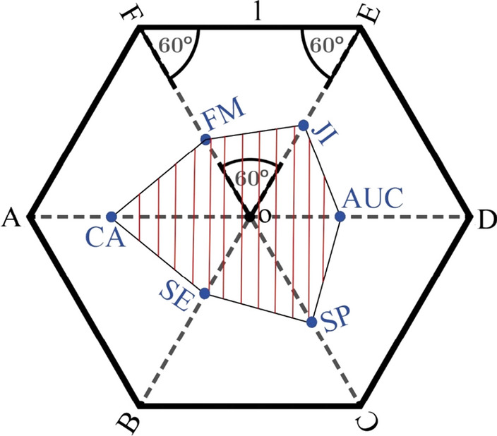
Polygon area metric

In Aydemir (2020) the polygon area metric (PAM) was proposed to easily evaluate the performance of the classifiers with a single value. PAM summarizes a total of six metrics as the classifier's accuracy rate, sensitivity, specificity, the area under curve (AUC), Jaccard index (JI), and F-measure as a single value. The working principle of PAM appears in Fig. 2. Each radius of a regular hexagon with a diameter of 2 units is allocated to each metric. In this case, each radius’s length will be 1 unit. The value of each metric, that is between [0 1], is signed on a radius by a point; in this way, the area of the formed hexagon is calculated. This area is normalized to [0 1] by dividing the area of the regular hexagon.

Fig. 2.

The polygon created by six system metrics in a regular hexagon (Aydemir 2020)

Inspired by this metric, we propose two polygons for sleep staging systems called the sensitivity polygon and general polygon. By using these polygons, two new metrics are introduced for outlining sleep staging systems.

Normalized area of sensitivity polygon (NAoSP)

A sensitivity polygon is created by the sensitivities of sleep stages’. In the six-stage sleep classification case, this polygon will be a regular hexagon. In the five-stage, four-stage, and three-stage cases, it will be in the form of a pentagon, square, and triangle, respectively. NAoSP is obtained by dividing the area of the polygon formed by the sensitivity values of the system by the area of the regular polygon. In this way, not only the sensitivity value of the sleep staging systems to the NREM1 stage, but also the sensitivity value of all the stages can be compared with a single value. The important point is that it is not possible to calculate NAoSP for a two-stage sleep classification case.

Normalized area of general polygon (NAoGP)

The sleep stages’ sensitivities, accuracy rate, and Cohen’s kappa coefficient constitute the general polygon. In the six-stage sleep classification case, this polygon will be a regular octagon. For the five-stage, four-stage, three-stage, and two-stage cases, it will be in the form of a heptagon, hexagon, pentagon, and square, respectively. By dividing the area of the polygon formed by the mentioned system metrics by the area of the regular polygon, the NAoGP could be calculated. Contrary to NAoSP, this parameter can be calculated for all cases. In this way, one can compare sleep staging systems with a single value in all dimensions instead of just the accuracy rate or Cohen’s kappa coefficient. A pseudo-code for calculating these metrics was presented as follows.

• X = {X₁, X₂, …, X_N}, Sequence of metrices such as kappa, ACC, and stages’ sensitivities.

• Irregular polygon area = 0.5 sin(2π/N) (X₁X₂ + X₂X₃ + ⋯ + X_NX₁).

• Regular polygon area = 0.5 N sin(2π/N).

• NAoSP or NAoGP = Irregular polygon area/ Regular polygon area.

Strategies in the evaluation of sleep stage classification systems

Evaluation of the sleep staging systems is generally performed based on two popular strategies: K-fold cross-validation (K-FCV) strategy and holdout strategy.

K-fold cross-validation (K-FCV) strategy

K-FCV is one of the most commonly adopted criteria for evaluating a model's performance and choosing a hypothesis. The advantage of this method over simple training and testing set splitting is that all the available data are used repeatedly to create a learning machine. Therefore, K-FCV reduces the risk of unlucky splitting. Based on this method, studies divide random data into K equal subsets. Each subset is used once as the test data and the remaining K-1 subsets are used as training data (Kayikcioglu et al. 2015). A common problem is to determine the number of folds that the training set should divide.

Holdout strategy

The holdout strategy is widely used in sleep staging studies (Zhu et al. 2014; Hassan and Bhuiyan 2017; Ghimatgar et al. 2019) to evaluate the performance of the systems. In this strategy, the data set is divided into two parts of training and testing sets. The classifier is given training with the training set, and the model is created and tested on the test data set. In general, researchers create training and testing sets by blending the data set several times to show the stability of the systems. In this case, the averages of all metrics are computed for the system.

Results

Classifier selection

Using the Diagnostic Feature Designer app., after extracting a total of 23 features, features were transferred to the Classification Learner app. to determine the best classifier. All classifiers in the application were tested with the 50-fold cross-validation strategy in which the data are divided into 50 parts, without overlapping. In each iteration, 49 parts are utilized for training and 1 part for testing. All parts are employed for testing once, and the accuracy rate is calculated. In this step, all parameters of classifiers are default parameters.

As mentioned previously, the EEG in the sleep-EDF data set was recorded from two different channels. According to the results of some previous studies, the results of the Pz-Oz channel are higher than the Fpz-Cz channel (Mousavi et al. 2019; Hassan and Bhuiyan 2017), and in some studies, the reverse of this was proved (Ghimatgar et al. 2019; Seifpour et al. 2018). For this, in the first step, both channels were considered in this study. The accuracy rates and learning times of the classifiers are given in Table 5 for both channels. The experiment was done on a laptop with an Intel Pentium^® 5 processor with 2.67 GHz and 5 GB RAM.

Table 5.

ACC and training time of the classifiers with the 50-fold cross-validation strategy; the highest value in each channel is indicated in boldface

Classifier	Methods	Pz-Oz		Fpz-Cz
		ACC	Training time (s)	ACC	Training time (s)
Decision trees	Fine tree	86.5	24.57	84.1	30.01
	Medium tree	83.3	15.61	81.2	30.58
	Coarse tree	74.5	11.92	70.1	51.37
Discriminant analysis	Linear discriminant	74.1	12.49	73.7	9.96
	Quadratic discriminant	51.7	9.01	53.3	10.13
Naive Bayes	Gaussian naive Bayes	38.3	15.52	43.9	18.49
	Kernel naive Bayes	73.8	427.55	64.2	574.86
Nearest neighbors	Fine KNN	74.5	21.43	75.2	37.64
	Medium KNN	78.4	18.75	77.3	22.90
	Coarse KNN	74.9	21.44	72.6	30.39
	Cosine KNN	77.5	20.49	76.3	71.96
	Cubic KNN	77.4	623.69	76.9	708.7
	Weighted KNN	78.9	20.74	78.3	37.69
Ensemble	Boosted tree	85.2	415.07	82.9	557.02
	Bagged tree	88.9	237.74	88.2	320.8
	Subspace discriminant	69.1	62.36	68.1	135.23
	Subspace KNN	83.8	292.51	76.7	470.2
	Rusboosted	77.4	159.21	74.5	423.4
Support vector machines	Linear SVM	–	–	–	–
	Quadratic SVM	–	–	–	–
	Cubic SVM	–	–	–	–
	Coarse Gaussian SVM	75.5	589.62	75.5	657.94
	Medium Gaussian SVM	84.5	484.78	84.2	504.19
	Fine Gaussian SVM	85.2	899.12	–	–

As seen in Table 5, in many classifiers, the ACC of the Pz-Oz channel is better than the ACC of the Fpz-Cz channel. For this, only Pz-Oz channel was used in the continuation of the study. Evidently, the “Bagged Tree” classifier from the “Ensemble Classifier” category outperforms both in terms of accuracy rate and time. Accordingly, this classifier was chosen for the continuation of the study. The default number of learners in this classifier is 30. In addition, the accuracy rate calculation of the classifiers whose training periods exceeded 15 min was stopped because, in the classification of sleep stages, classifiers are required to be fast, especially for real-time sleep scoring (Ghimatgar et al. 2019).

Feature set evaluation

Considering the order of the Kruskal–Wallis and ANOVA tests for the features, a simple path was followed to determine the feature set in the classification phase; by selecting only the best feature, classification was performed for the six-stage sleep classification case with the Bagged Tree classifier. Subsequently, the second-best feature was added, and the dataset was classified with just two features. In this way, the accuracy rates were calculated by adding only one feature to the selected features in each time. These accuracy rates and the features ranked based on statistical tests, from the most significant feature to the most insignificant feature, are presented in Table 6. In this step, the default number of learners in this classifier was used.

Table 6.

Evaluation and ranking of the extracted features with the Kruskal–Wallis test and ANOVA; the highest value in each method is indicated in boldface

Order	Kruskal–Wallis	ACC	ANOVA	ACC
1	Beta 2	60.7	SNR	41.3
2	Theta 2	81.7	Crest factor	48.9
3	Theta	84.8	SINAD	52.5
4	Theta	84.8	Delta 1	64.4
5	Delta 1	86.2	Theta 2	72.0
6	Beta 1	88.0	Delta	74.2
7	All bands	87.9	Beta 2	86.2
8	Standard deviation	88.1	Impulse factor	86.4
9	Delta	88.1	Clearance factor	85.7
10	RMS	88.1	Skewness	86.0
11	Crest factor	88.6	Delta 2	86.5
12	Impulse factor	88.6	Alpha	86.5
13	Clearance factor	88.5	Standard deviation	87.4
14	SNR	88.0	RMS	88.0
15	Peak value	88.0	Beta 1	88.9
16	SINAD	88.3	Peak value	88.9
17	Delta 2	88.4	Shape factor	88.8
18	Kurtosis	88.5	Mean	89.6
19	Alfa	89.0	Kurtosis	89.5
20	Shape factor	88.9	Theta 1	89.1
21	Skewness	88.9	Theta	89.3
22	Mean	89.2	All bands	89.0
23	THD	88.9	THD	88.8

As can be seen in this table, based on the order of the features given by the Kruskal–Wallis test, the Bagged Tree classifier has classified six stages with an accuracy rate of 60.6%, using only the most significant feature (Beta 2). When the second significant feature was added, the accuracy rate increased to 82.3%. With the addition of the features, the highest test accuracy rate was obtained with 22 features. The confusion matrix of this experiment with an 89.2% accuracy rate is given in Table 7.

Table 7.

Confusion matrix of classification using the first 22 features based on the Kruskal–Wallis test (ACC = 89.2); the number of correctly predicted epochs and sensitivity of each stage are indicated in boldface

	S1	S2	S3	S4	R	W	Sen
S1	177	114	2	3	144	164	29.3
S2	30	3292	113	14	105	67	90.9
S3	5	207	359	88	2	11	53.4
S4	3	18	102	500	0	4	79.7
R	46	213	0	1	1282	67	79.7
W	50	24	5	3	30	7919	98.6

According to the ANOVA’s ranking, the highest accuracy rate was obtained by using 18 features, and its ACC is around 89.6%. Thus, for the continuation of the study, the first 18 features were selected as the best feature set in the order given by ANOVA. The confusion matrix of this experiment is given in Table 8.

Table 8.

Confusion matrix of classification using the first 18 features based on ANOVA (ACC = 89.6); the number of correctly predicted epochs and sensitivity of each stage are indicated in boldface

	S1	S2	S3	S4	R	W	Sen
S1	183	95	3	1	158	164	30.3
S2	20	3305	105	18	102	71	91.3
S3	5	216	370	68	2	11	55.1
S4	2	19	98	501	2	5	79.9
R	51	186	0	1	1306	65	81.2
W	47	27	3	0	29	7925	98.7

It is worth mentioning that all confusion matrices of this step based on Kruskal–Wallis test and the ANOVA were provided in the electronic supplementary material.

Evaluation of the proposed system

Both strategies in sleep stage classification systems based on K-FCV and holdout were used. More information on how these evaluations were performed as well as results is given below.

System evaluation by K-fold cross-validation strategy

In this strategy, the number of folds was selected as 50. Using the first 18 features based on ANOVA, five different numbers of learners were tested for the Bagged Tree classifier, namely 100, 200, 300, 400, and 500. The results appear in Table 9. As seen in Table, when the number of learners is selected as 400, the highest NAoSP and NAoGP values are obtained. In Table 10, the confusion matrix of the procedure is given.

Table 9.

Results of the 50-fold cross-validation strategy with different numbers of learners in Bagged Tree classifier; the highest value in each metric is indicated in boldface

Metrics\number of learner	100	200	300	400	500
Kappa	0.8480	0.8489	0.8475	0.8495	0.8493
ACC	0.9035	0.9041	0.9033	0.9044	0.9044
Sen. S1	0.2980	0.2864	0.2864	0.3029	0.2897
Sen. S2	0.9229	0.9218	0.9204	0.9199	0.9201
Sen. S3	0.5669	0.5714	0.5550	0.5744	0.5684
Sen. S4	0.8086	0.8070	0.8197	0.8213	0.8197
Sen. R	0.8272	0.8346	0.8297	0.8272	0.8346
Sen. W	0.9912	0.9920	0.9924	0.9930	0.9922
NAoSP	0.5068	0.5062	0.5029	0.5134	0.5092
NAoGP	0.5777	0.5777	0.5748	0.5832	0.5801

Table 10.

Confusion matrix of the 50-fold cross-validation strategy with 400 learners in Bagged Tree classifier (ACC = 0.9044); the number of correctly predicted epochs and sensitivity of each stage are indicated in boldface

	S1	S2	S3	S4	R	W	Sen
S1	186	105	1	0	147	165	0.3029
S2	19	3331	98	13	93	67	0.9199
S3	3	191	386	77	2	13	0.5744
S4	2	19	82	515	2	7	0.8213
R	36	175	0	1	1331	66	0.8272
W	21	12	2	1	20	7975	0.9930

System evaluation by holdout strategy

Generally, studies that used the sleep-EDF data set employed half of all sleep stages as a training and the other half as a testing set. In order to compare the results of the proposed system with those of the literature, the same procedure was adopted in the present study. The number of epochs in the training and testing sets for each stage is presented in Table 1. For system evaluation by the holdout strategy, the Bagged Tree classifier, whose number of learners was selected as 200, was trained by the 50-fold cross-validation strategy, and the metrics in the test phase were calculated. The results of this process, which was repeated ten times, are given in Table 11 for the six-stage classification case. The repetition results of five-stage, four-stage, three-stage, and two-stage cases (ten times) are given in Appendix in Tables 16, 17, 18, and 19, respectively. In addition, the average values of all metrics were calculated in the last row of each table.

Table 11.

The results of ten repetitions for the six-stage classification case; average of ten repetitions for each metric is indicated in boldface 

Iteration	Kappa	ACC	Sen. S1	Sen. S2	Sen. S3	Sen. S4	Sen. R	Sen. W	NAoSP	NAoGP
1	0.8356	0.8957	0.2350	0.9193	0.5386	0.7961	0.8161	0.9882	0.4715	0.5477
2	0.8401	0.8988	0.2615	0.9249	0.5029	0.8025	0.8211	0.9912	0.4738	0.5508
3	0.8347	0.8955	0.2251	0.9243	0.5208	0.7866	0.8074	0.9905	0.4595	0.5387
4	0.8383	0.8975	0.2483	0.9149	0.5416	0.8535	0.8037	0.9905	0.4855	0.5591
5	0.8391	0.8982	0.2218	0.9199	0.5625	0.8025	0.8223	0.9900	0.4777	0.5538
6	0.8398	0.8986	0.2615	0.9188	0.5029	0.8184	0.8211	0.9922	0.4767	0.5530
7	0.8344	0.8954	0.2649	0.9182	0.5208	0.7898	0.7962	0.9920	0.4690	0.5454
8	0.8288	0.8916	0.2450	0.9204	0.5386	0.7770	0.7776	0.9885	0.4592	0.5362
9	0.8434	0.9008	0.2814	0.9210	0.5208	0.8439	0.8223	0.9902	0.4942	0.5669
10	0.8457	0.9020	0.2913	0.9304	0.5952	0.8184	0.7987	0.9880	0.5071	0.5770
Avg.	0.8380	0.8974	0.2536	0.9212	0.5345	0.8089	0.8086	0.9901	0.4774	0.5529

Table 16.

The results of ten repetitions for the five-stage classification case; average of ten repetitions for each metric is indicated in boldface

Iteration	Kappa	ACC	Sen. S1	Sen. S2	Sen. S3 + S4	Sen. R	Sen. W	NAoSP	NAoGP
1	0.8546	0.9080	0.2450	0.9144	0.8169	0.8173	0.9880	0.5377	0.6127
2	0.8543	0.9082	0.2516	0.9133	0.8092	0.8074	0.9915	0.5344	0.6106
3	0.8536	0.9079	0.2152	0.9226	0.8076	0.8049	0.9902	0.5208	0.6010
4	0.8571	0.9098	0.2748	0.9055	0.8307	0.8149	0.9912	0.5516	0.6236
5	0.8601	0.9119	0.2417	0.9171	0.8369	0.8248	0.9895	0.5470	0.6216
6	0.8583	0.9107	0.2384	0.9182	0.8092	0.8248	0.9915	0.5367	0.6139
7	0.8530	0.9075	0.2615	0.9077	0.8138	0.8037	0.9920	0.5374	0.6122
8	0.8479	0.9041	0.2450	0.9144	0.8107	0.7788	0.9892	0.5219	0.5992
9	0.8584	0.9107	0.2847	0.9144	0.8138	0.8136	0.9912	0.5511	0.6236
10	0.8577	0.9102	0.2582	0.9177	0.8476	0.7950	0.9890	0.5461	0.6199
Avg.	0.8555	0.9089	0.2517	0.9146	0.8197	0.8086	0.9904	0.5385	0.6139

Table 17.

The results of ten repetitions for the four-stage classification case; average of ten repetitions for each metric is indicated in boldface

Iteration	Kappa	ACC	Sen. S1 + S2	Sen. S3 + S4	Sen. R	Sen. W	NAoSP	NAoGP
1	0.8596	0.9133	0.8703	0.8167	0.7565	0.9830	0.7320	0.7496
2	0.8581	0.9124	0.8646	0.8123	0.7540	0.9855	0.7275	0.7459
3	0.8521	0.9088	0.8570	0.8107	0.7354	0.9868	0.7156	0.7352
4	0.8514	0.9080	0.8580	0.8307	0.7428	0.9800	0.7247	0.7408
5	0.8589	0.9131	0.8608	0.8123	0.7639	0.9868	0.7308	0.7486
6	0.8616	0.9146	0.8674	0.7969	0.7701	0.9875	0.7305	0.7497
7	0.8561	0.9112	0.8551	0.8184	0.7527	0.9875	0.7260	0.7440
8	0.8506	0.9079	0.8717	0.7923	0.7192	0.9835	0.7063	0.7280
9	0.8549	0.9104	0.8613	0.8123	0.7552	0.9833	0.7257	0.7431
10	0.8561	0.9111	0.8698	0.8400	0.7242	0.9818	0.7260	0.7438
Avg.	0.8560	0.9111	0.8637	0.8143	0.7475	0.9846	0.7246	0.7429

Table 18.

The results of ten repetitions for the three-stage classification case; average of ten repetitions for each metric is indicated in boldface

Iteration	Kappa	ACC	Sen. NREM	Sen. R	Sen. W	NAoSP	NAoGP
1	0.8887	0.9364	0.9207	0.7664	0.9813	0.7871	0.8048
2	0.8923	0.9385	0.9250	0.7515	0.9853	0.7824	0.8041
3	0.8888	0.9367	0.9218	0.7416	0.9860	0.7746	0.7974
4	0.8946	0.9398	0.9283	0.7639	0.9830	0.7909	0.8106
5	0.8889	0.9365	0.9160	0.7639	0.9853	0.7850	0.8037
6	0.8917	0.9382	0.9207	0.7602	0.9860	0.7858	0.8059
7	0.8932	0.9390	0.9218	0.7677	0.9853	0.7907	0.8097
8	0.8846	0.9342	0.9247	0.7304	0.9815	0.7667	0.7902
9	0.8928	0.9388	0.9225	0.7726	0.9833	0.7932	0.8109
10	0.8854	0.9345	0.9283	0.7279	0.9803	0.7664	0.7905
Avg.	0.8901	0.9373	0.9230	0.7547	0.9838	0.7823	0.8028

Table 19.

The results of ten repetitions for the two-stage classification case; average of ten repetitions for each metric is indicated in boldface

Iteration	Kappa	ACC	Sen. sleep	Sen. W	NAoGP
1	0.9483	0.9742	0.9680	0.9798	0.9362
2	0.9480	0.9741	0.9663	0.9810	0.9358
3	0.9388	0.9695	0.9613	0.9768	0.9246
4	0.9420	0.9711	0.9674	0.9743	0.9287
5	0.9422	0.9712	0.9621	0.9793	0.9286
6	0.9443	0.9723	0.9624	0.9810	0.9311
7	0.9435	0.9719	0.9607	0.9818	0.9301
8	0.9430	0.9716	0.9677	0.9750	0.9299
9	0.9430	0.9716	0.9638	0.9785	0.9297
10	0.9367	0.9684	0.9663	0.9703	0.9224
Avg	0.9430	0.9716	0.9646	0.9778	0.9297

The proposed hybrid system

The classification of the NREM1 stage is a common problem of all sleep scoring systems and a research challenge in this domain (Hassan and Bhuiyan 2016). From a neurophysiological point of view, the NREM1 stage is a transition phase. Since this stage is a mixture of wakefulness and sleep, it is similar to the neuronal oscillations of wakefulness. In the case of REM, the cortex shows gamma waves of 40–60 Hz as in the wake stage (Horne 2013). Due to these similarities, NREM1 is misclassified as wake or REM both in computerized sleep scoring methods and by human expert scorers (Hassan and Bhuiyan 2016).

When looking at the six-stage case confusion matrix of the system proposed in this study, it is seen that most of the epochs in the NREM1 stage are mistakenly classified as wake or REM. This problem also exists between NREM2 and NREM3. Most of the epochs in the NREM2 stage are mistakenly classified as NREM3 and vice versa. To reduce the impact of these problems, in addition to the six-stage sleep classification system called the mother system, we trained two binary systems using the training data set, NREM1 and wake and NREM2 and NREM3 called minor1 and minor2 systems, respectively. In this case, epochs tagged as an NREM1 or wake by the mother system are again classified with the minor1 system. Furthermore, epochs tagged as an NREM2 or NREM3 by the mother system are once again classified with the minor2 system. The flowchart of this hybrid system is demonstrated in Fig. 3.

Fig. 3.

Flowchart of the proposed mother system and hybrid system

For the six-stage case, the results of the hybrid system are given in Table 12. In addition, Fig. 4 presents the changes in the results between mother and hybrid systems. Evidently, in the hybrid system, the NREM1 sensitivity increased from 25.36% to 32.48%. There is an 8% and 1% increase in the sensitivity of NREM3 and NREM2, respectively. There is little decrease in the wake stage. Nevertheless, when we look at the NAoSP and NAoGP of both systems, it seems clear that the hybrid system is superior. There is a 4% increase in both the sensitivity of the hybrid system and the overall evaluation of the system.

Table 12.

The results of ten repetitions for the six-stage sleep classification case obtained by the proposed hybrid system; average of ten repetitions for each metric is indicated in boldface

Iteration	Kappa	ACC	Sen. S1	Sen. S2	Sen. S3	Sen. S4	Sen. R	Sen. W	NAoSP	NAoGP
1	0.8475	0.9030	0.2682	0.9337	0.6250	0.7961	0.8086	0.9875	0.5065	0.5773
2	0.8496	0.9046	0.3013	0.9348	0.5833	0.8025	0.8074	0.9907	0.5069	0.5782
3	0.8413	0.8975	0.3344	0.9160	0.6398	0.8089	0.7888	0.9843	0.5256	0.5885
4	0.8482	0.9034	0.3079	0.9320	0.5982	0.8535	0.7900	0.9875	0.5189	0.5864
5	0.8518	0.9059	0.2913	0.9353	0.6250	0.8025	0.8136	0.9890	0.5174	0.5868
6	0.8538	0.9073	0.3211	0.9359	0.5892	0.8184	0.8111	0.9912	0.5201	0.5893
7	0.8488	0.9037	0.3576	0.9348	0.6428	0.7961	0.7950	0.9828	0.5354	0.5982
8	0.8456	0.9004	0.3708	0.9287	0.6339	0.8152	0.7689	0.9853	0.5333	0.5954
9	0.8545	0.9075	0.3609	0.9320	0.5982	0.8439	0.8000	0.9900	0.5372	0.6018
10	0.8552	0.9079	0.3344	0.9425	0.6547	0.8184	0.7888	0.9875	0.5371	0.6022
Avg.	0.8496	0.9041	0.3248	0.9325	0.6190	0.8155	0.7972	0.9875	0.5238	0.5904

Fig. 4.

Comparison of the mother and hybrid systems' results for the six-stage case

For the five-stage case, we also trained two minor binary systems: NREM1 and wake and NREM2 and (NREM3 + NREM4) called minor 1 and minor 2, respectively. In this case, epochs tagged as an NREM1 or wake by the mother system were again classified with the minor1 system, and epochs tagged as an NREM2 or (NREM3 + NREM4) by the mother system were again classified with the minor2 system. The comparison of the results between the mother system and the hybrid system is given in Fig. 5. There is a 3% increase in NAoSP and a > 2% increase in NAoGP. In addition, the results of this experiment, repeated ten times, are presented in Table 20.

Fig. 5.

Comparison of the mother and hybrid systems' results for the five-stage case

Table 20.

The results of ten repetitions for the five-stage sleep classification case obtained by the proposed hybrid system; average of ten repetitions for each metric is indicated in boldface

Iteration	Kappa	ACC	Sen. S1	Sen. S2	Sen. S3 + S4	Sen. R	Sen. W	NAoSP	NAoGP
1	0.8640	0.9138	0.2715	0.9304	0.8553	0.8037	0.9863	0.5593	0.6312
2	0.8672	0.9161	0.3211	0.9298	0.8507	0.7937	0.9897	0.5737	0.6425
3	0.8654	0.9152	0.2781	0.9409	0.8430	0.7888	0.9885	0.5549	0.6288
4	0.8682	0.9165	0.3112	0.9215	0.8769	0.8049	0.9885	0.5808	0.6479
5	0.8714	0.9187	0.3013	0.9331	0.8692	0.8136	0.9877	0.5801	0.6488
6	0.8683	0.9169	0.2880	0.9331	0.8384	0.8099	0.9910	0.5637	0.6362
7	0.8612	0.9124	0.3079	0.9210	0.8507	0.7900	0.9885	0.5649	0.6340
8	0.8554	0.9087	0.2682	0.9265	0.8446	0.7652	0.9880	0.5396	0.6142
9	0.8684	0.9167	0.3509	0.9282	0.8523	0.7913	0.9897	0.5843	0.6503
10	0.8692	0.9173	0.3046	0.9353	0.8876	0.7826	0.9870	0.5766	0.6453
Avg.	0.8659	0.9153	0.3003	0.9300	0.8569	0.7944	0.9885	0.5678	0.6380

For the four-stage case, we trained a binary system, (NREM1 + NREM2) and REM. The comparison of the results is illustrated in Fig. 6. By looking at the results, we can see that the effect of the hybrid system appears to be small for this experiment. In addition, the results of this stage, repeated ten times, are shown in Table 21.

Fig. 6.

Comparison of the mother and hybrid systems' results for the four-stage case

Table 21.

The results of ten repetitions for the four-stage sleep classification case obtained by the proposed hybrid system; average of ten repetitions for each metric is indicated in boldface

Iteration	Kappa	ACC	Sen. S1 + S2	Sen. S3 + S4	Sen. R	Sen. W	NAoSP	NAoGP
1	0.8599	0.9135	0.8665	0.8169	0.7677	0.9830	0.7354	0.7520
2	0.8630	0.9154	0.8712	0.8123	0.7652	0.9855	0.7355	0.7536
3	0.8563	0.9115	0.8655	0.8107	0.7378	0.9868	0.7205	0.7404
4	0.8561	0.9109	0.8641	0.8307	0.7540	0.9800	0.7325	0.7482
5	0.8605	0.9140	0.8613	0.8123	0.7714	0.9868	0.7343	0.7517
6	0.8646	0.9165	0.8707	0.7969	0.7788	0.9875	0.7359	0.7547
7	0.8601	0.9137	0.8613	0.8184	0.7602	0.9875	0.7321	0.7500
8	0.8513	0.9083	0.8698	0.7923	0.7279	0.9835	0.7093	0.7304
9	0.8606	0.9140	0.8679	0.8123	0.7714	0.9833	0.7359	0.7527
10	0.8613	0.9142	0.8726	0.8400	0.7465	0.9818	0.7375	0.7540
Avg.	0.8594	0.9133	0.8672	0.8143	0.7581	0.9846	0.7309	0.7488

We also trained a single binary system for the three-stage case, NREM and REM. The comparison of the results of the two proposed systems is given in Fig. 7. In this experiment, there is a 2% increase in both the sensitivity of the hybrid system and the overall evaluation. In addition, the results of this stage, repeated ten times, are given in Table 22.

Fig. 7.

Comparison of the mother and hybrid systems' results for the three-stage case

Table 22.

The results of ten repetitions for the three-stage sleep classification case obtained by the proposed hybrid system; average of ten repetitions for each metric is indicated in boldface

Iteration	Kappa	ACC	Sen. NREM	Sen. R	Sen. W	NAoSP	NAoGP
1	0.8905	0.9372	0.9109	0.8074	0.9813	0.8072	0.8180
2	0.8966	0.9407	0.9174	0.7987	0.9853	0.8079	0.8220
3	0.8940	0.9394	0.9142	0.7937	0.9860	0.8032	0.8177
4	0.9000	0.9427	0.9232	0.8086	0.9830	0.8164	0.8290
5	0.8963	0.9405	0.9058	0.8360	0.9853	0.8245	0.8318
6	0.8978	0.9414	0.9109	0.8236	0.9860	0.8202	0.8301
7	0.8955	0.9402	0.9163	0.7975	0.9853	0.8065	0.8205
8	0.8869	0.9352	0.9153	0.7726	0.9815	0.7880	0.8043
9	0.8950	0.9398	0.9145	0.8099	0.9833	0.8121	0.8236
10	0.8936	0.9390	0.9236	0.7863	0.9803	0.8008	0.8159
Avg.	0.8947	0.9397	0.9153	0.8035	0.9838	0.8087	0.8213

The sensitivity polygons and general polygons of the six-stage, five-stage, four-stage, and three-stage cases of the hybrid systems are depicted in Figs. 8 and 9, respectively. The general polygon formed for the two-stage case was obtained from the proposed mother system.

Fig. 8.

Sensitivity polygons of the hybrid systems, a six-stage case, b five-stage case, c four-stage case, d three-stage case

Fig. 9.

General polygons of the hybrid systems for the six-stage (a), five-stage (b), four-stage (c), three-stage case (d), and the general polygon of the mother system for the two-stage case (e)

Discussion

To evaluate the state-of-the-art methods in the literature and compare them with the proposed systems, we calculated NAoSP and NAoGP metrics by confusion matrices given in these studies. In many studies, confusion matrices are given for only six-stage cases and five-stage cases. Thus, it is not possible to calculate the NAoSP and NAoGP metrics for other stage cases.

As mentioned before, some studies used the K-FCV strategy for evaluation of the systems. For four recent studies based on this strategy, NAoSP and NAoGP metrics were calculated by the given confusion matrices for the six-stage case. The results are presented in Table 13. Evidently (Sharma et al. 2019a) has high values in all metrics except for wake and NREM2 sensitivities. The proposed system has high values in NAoSP and NAoGP metrics compared to (Sharma et al. 2017) and (Ghimatgar et al. 2019). Also, the wake sensitivity of our proposed system is higher than that of the other systems. As mentioned previously, at this step, we used the 50-fold cross-validation strategy with 400 learners in the Bagged Tree classifier.

Table 13.

The average metrics of the proposed systems and the other state-of-the-art methods based on the K-fold cross-validation strategy for the six-stage sleep classification case; the highest value in each metric is indicated in boldface

Approach	Kappa	ACC	Sen. S1	Sen. S2	Sen. S3	Sen. S4	Sen. R	Sen. W	NAoSP	NAoGP
Sharma et al. (2019a)	0.8680	0.9149	0.6492	0.8835	0.6507	0.8771	0.8401	0.9851	0.6594	0.6942
Sharma et al. (2017)	0.8429	0.9002	0.1887	0.9251	0.5238	0.8325	0.8365	0.9923	0.4682	0.5420
Ghimatgar et al. (2019)	0.7601	0.8473	0.1092	0.8657	0.1654	0.6602	0.8178	0.9723	0.2981	0.3853
Proposed sistem	0.8495	0.9044	0.3029	0.9199	0.5744	0.8213	0.8272	0.9930	0.5134	0.5832

For recent studies based on the holdout strategy, Table 14 is prepared for the six-stage case. For the sake of comparison, the metrics calculated for the proposed mother and hybrid systems are given in this table. The highest NAoSP and NAoGP values calculated for (Mousavi et al. 2019)’s study were 0.7196 and 0.7368, respectively. This study was conducted using Deep Learning methods. However, in studies implemented by machine learning methods, our proposed hybrid system has the highest NAoGP value (%59.04) that it is about %1 more than NAoGP of (Hassan and Bhuiyan 2017) which has a maximum value (%58.28) of literature review. It means that the proposed system is more successful than the existing systems when viewed from all dimensions. Also, our system’s ACC, Cohen’s kappa coefficient, and sensitivity of NREM2 is higher than other studies. In addition, the wake sensitivity of the proposed mother system has the highest value (%99.01) among the existing machine learning and Deep Learning systems.

Table 14.

The average metrics of the proposed systems and the other state-of-the-art methods based on the holdout strategy for the six-stage sleep classification case; the highest value in each metric in machine learning algorithms is indicated in boldface

Method	Approach	Kappa	ACC	Sen. S1	Sen. S2	Sen. S3	Sen. S4	Sen. R	Sen. W	NAoSP	NAoGP
Deep learning algorithms	Mousavi et al. (2019)	0.8624	0.9096	0.6788	0.8292	0.8303	0.8306	0.9577	0.9662	0.7196	0.7368
Machine learning algorithms	Seifpour et al. (2018)	0.8207	0.8859	0.1920	0.9088	0.4107	0.7579	0.8422	0.9860	0.4195	0.4973
	Hassan and Bhuiyan (2016)	0.7967	0.8688	0.4735	0.8901	0.7827	0.3885	0.7838	0.9505	0.4846	0.5331
	Hassan et al. (2015a)	0.7638	0.8501	0.2450	0.8387	0.4434	0.7929	0.6906	0.9709	0.4235	0.4697
	Hassan et al. (2015b)	0.6889	0.8034	0.2152	0.8155	0.3541	0.6146	0.5652	0.9419	0.3191	0.3636
	Hassan and Subasi (2017)	0.8360	0.8962	0.3741	0.9287	0.3452	0.8407	0.8223	0.9858	0.4842	0.5462
	Hassan and Bhuiyan (2017)	0.7767	0.8543	0.4205	0.7951	0.8660	0.4808	0.8049	0.9515	0.5002	0.5389
	Hassan and Bhuiyan (2017)	0.8434	0.9000	0.4072	0.9077	0.4821	0.8184	0.8335	0.9880	0.5289	0.5828
	Hassan and Bhuiyan (2016)	0.8434	0.9004	0.3874	0.9177	0.5059	0.7770	0.8360	0.9865	0.5213	0.5772
	Hassan and Bhuiyan (2016)	0.8209	0.8863	0.3907	0.9044	0.4255	0.8216	0.7850	0.9793	0.4947	0.5475
	Proposed mother system	0.8380	0.8974	0.2536	0.9212	0.5345	0.8089	0.8086	0.9901	0.4774	0.5529
	Proposed hybrid system	0.8496	0.9041	0.3248	0.9325	0.6190	0.8155	0.7972	0.9875	0.5238	0.5904

The metrics calculated for the five-stage case based on confusion matrices are given in Table 15. As can be seen, (Hassan and Bhuiyan 2016)’s study has the highest NAoSP and NAoGP value.

Table 15.

The average metrics of the proposed systems and the other state-of-the-art methods based on the holdout strategy for the five-stage sleep classification case; the highest value in each metric is indicated in boldface

Approach	Kappa	ACC	Sen. S1	Sen. S2	Sen. S3 + S4	Sen. R	Sen. W	NAoSP	NAoGP
Hassan and Bhuiyan (2016)	0.8616	0.9125	0.3741	0.9144	0.8107	0.8211	0.9868	0.6002	0.6470
Hassan and Bhuiyan (2017)	0.8639	0.9136	0.3973	0.9022	0.8230	0.8298	0.9888	0.6130	0.6578
Hassan and Bhuiyan (2016)	0.8438	0.9011	0.3973	0.8956	0.7984	0.7813	0.9820	0.5866	0.6286
Hassan and Bhuiyan (2016)	0.8550	0.9069	0.4701	0.9237	0.9000	0.8086	0.9528	0.6548	0.6838
Hassan et al. (2015a)	0.7794	0.8604	0.2748	0.8293	0.7692	0.6956	0.9659	0.4944	0.5329
Hassan et al. (2015b)	0.7169	0.8203	0.2284	0.8083	0.6738	0.6186	0.9339	0.4155	0.4507
Hassan and Subasi (2017)	0.8542	0.9079	0.3874	0.9061	0.7892	0.8136	0.9858	0.5923	0.6384
Proposed mother system	0.8555	0.9089	0.2517	0.9146	0.8197	0.8086	0.9904	0.5385	0.6139
Proposed hybrid system	0.8659	0.9153	0.3003	0.9300	0.8569	0.7944	0.9885	0.5678	0.6380

The main aim of the article is to introduce two new metrics for the evaluation of sleep staging systems. With the NAoSP metric, the sensitivity of the systems to all sleep stages can be measured with a single metric. Also, the NAoGP metric was introduced to compare systems from all dimensions. In this way, the gap in the comparison of these systems is filled by expressing many metrics with a single metric. The NAoGP metric can contain other metrics such as F-measure used in classification processes. In this way, sleep staging systems can be evaluated more comprehensively. Also, proposed metrics can be tested for sleep stages classification using optimal wavelets suggested in (Sharma et al. 2020).

In addition, in this study, a new sleep staging system without writing codes was proposed with two applications offered by MATLAB (2019b). The use of these applications causes some restrictions but eliminates errors in coding such as programmer's mistakes. The advantage of the proposed sleep scoring system is that it has higher ACC and Cohen’s kappa coefficient compared to those previously published using machine learning methods and is more successful than them based on the new NAoGP metric.

Conclusion

Evaluation of sleep stage classification systems is generally based on the accuracy rate. However, merely evaluating a system based on the accuracy rate is not synonymous with evaluating that system from all dimensions. For this purpose, the Cohen’s kappa coefficient of the systems and, in recent years, even the NREM1 sensitivity have been used as the system evaluation metrics. Nevertheless, a system may be more successful in one metric but show a poor performance for the other metric. Therefore, in this study, two new metrics for sleep staging systems were proposed, and the existing systems in the literature were evaluated accordingly. Also, a new method was introduced for the automatic classification of sleep stages. This method based on a single EEG channel was tested on the sleep-EDF dataset from the PhysioNet website bank. Two applications offered by MATLAB (2019b) were employed for the extraction and classification of the features after the pre-processing of the signals. Based on the NAoGP value, the proposed hybrid system in the six-stage case is more successful than the existing machine learning systems. Consequently, the proposed single-channel method can be adopted for a robust and reliable sleep stage classification based on all the dimensions required for real-time applications.

Compared to systems based on code writing, one of the problems in working with applications is that they are not able to change the parameters of the method as desired. This negatively affects the results of the studies. For example, although the Diagnostic Feature Designer application is easier to use than code writing, one does not have the opportunity to obtain the desired features in the frequency domain. Also, in using K-fold cross-validation strategy in Classification Learner app. maximum fold number could be selected 50 and, in this case, it is not possible to use Leave one-out cross-validation strategy. Therefore, the development of the proposed sleep staging system by using different feature extraction and classification methods, testing on different and bigger data sets, and comparison with NAoSP and NAoGP metrics with existing systems in the literature are planned as our future studies.

Electronic supplementary material

Below is the link to the electronic supplementary material.

Appendix

See Tables 16, 17, 18, 19, 20, 21 and 22.

References

- Akben SB, Alkan A. Visual interpretation of biomedical time series using Parzen window-based density-amplitude domain transformation. PLoS ONE. 2016 doi: 10.1371/journal.pone.0163569. [DOI] [PMC free article] [PubMed] [Google Scholar]
- Aydemir O. A new performance evaluation metric for classifiers: polygon area metric. J Classif. 2020 doi: 10.1007/s00357-020-09362-5. [DOI] [Google Scholar]
- Boashash B, Ouelha S. Automatic signal abnormality detection using time-frequency features and machine learning: a newborn EEG seizure case study. Knowl Based Syst. 2016;106:38–50. doi: 10.1016/j.knosys.2016.05.027. [DOI] [Google Scholar]
- Cohen J. A coefficient of agreement for nominal scales. Educ Psychol Meas. 1960;20(1):37–46. doi: 10.1177/001316446002000104. [DOI] [Google Scholar]
- Dhok S, Pimpalkhute V, Chandurkar A, Bhurane AA, Sharma M, Acharya UR. Automated phase classification in cyclic alternating patterns in sleep stages using Wigner–Ville distribution based features. Comput Biol Med. 2020;119:103691. doi: 10.1016/j.compbiomed.2020.103691. [DOI] [PubMed] [Google Scholar]
- Ghimatgar H, Kazemi K, Helfroush MS, Aarabi A. An automatic single-channel EEG-based sleep stage scoring method based on hidden Markov model. J Neurosci Methods. 2019;324:108320. doi: 10.1016/j.jneumeth.2019.108320. [DOI] [PubMed] [Google Scholar]
- Goldberger AL, et al. PhysioBank, PhysioToolkit, and PhysioNet: components of a new research resource for complex physiologic signals. Circulation. 2000 doi: 10.1161/01.cir.101.23.e215. [DOI] [PubMed] [Google Scholar]
- Hassan AR, Bhuiyan MIH. Computer-aided sleep staging using complete ensemble empirical mode decomposition with adaptive noise and bootstrap aggregating. Biomed Signal Process Control. 2016;24:1–10. doi: 10.1016/j.bspc.2015.09.002. [DOI] [Google Scholar]
- Hassan AR, Bhuiyan MIH. A decision support system for automatic sleep staging from EEG signals using tunable Q-factor wavelet transform and spectral features. J Neurosci Methods. 2016;271:107–118. doi: 10.1016/j.jneumeth.2016.07.012. [DOI] [PubMed] [Google Scholar]
- Hassan AR, Bhuiyan MIH. Automatic sleep scoring using statistical features in the EMD domain and ensemble methods. Biocybern Biomed Eng. 2016;36(1):248–255. doi: 10.1016/j.bbe.2015.11.001. [DOI] [Google Scholar]
- Hassan AR, Bhuiyan MIH. An automated method for sleep staging from EEG signals using normal inverse Gaussian parameters and adaptive boosting. Neurocomputing. 2017;219:76–87. doi: 10.1016/j.neucom.2016.09.011. [DOI] [Google Scholar]
- Hassan AR, Bhuiyan MIH. Automated identification of sleep states from EEG signals by means of ensemble empirical mode decomposition and random under sampling boosting. Comput Methods Programs Biomed. 2017;140:201–210. doi: 10.1016/j.cmpb.2016.12.015. [DOI] [PubMed] [Google Scholar]
- Hassan AR, Subasi A. A decision support system for automated identification of sleep stages from single-channel EEG signals. Knowl Based Syst. 2017;128:115–124. doi: 10.1016/j.knosys.2017.05.005. [DOI] [Google Scholar]
- Hassan AR, Bashar SK, Bhuiyan MIH (2015) On the classification of sleep states by means of statistical and spectral features from single channel electroencephalogram. In: 2015 international conference on advances in computing, communications and informatics, ICACCI 2015, pp 2238–2243. 10.1109/ICACCI.2015.7275950
- Hassan AR, Bashar SK, Bhuiyan MIH (2016) Automatic classification of sleep stages from single-channel electroencephalogram. In: 12th IEEE international conference electronics, energy, environment, communication, computer, control: (E3-C3), INDICON 2015.10.1109/INDICON.2015.7443756
- Horne J. Why REM sleep? Clues beyond the laboratory in a more challenging world. Biol Psychol. 2013;92(2):152–168. doi: 10.1016/j.biopsycho.2012.10.010. [DOI] [PubMed] [Google Scholar]
- Hsu YL, Yang YT, Wang JS, Hsu CY. Automatic sleep stage recurrent neural classifier using energy features of EEG signals. Neurocomputing. 2013;104:105–114. doi: 10.1016/j.neucom.2012.11.003. [DOI] [Google Scholar]
- Kayikcioglu T, Maleki M, Eroglu K. Fast and accurate PLS-based classification of EEG sleep using single channel data. Expert Syst Appl. 2015;42(21):7825–7830. doi: 10.1016/j.eswa.2015.06.010. [DOI] [Google Scholar]
- Kemp B, Zwinderman AH, Tuk B, Kamphuisen HAC, Oberyé JJL. Analysis of a sleep-dependent neuronal feedback loop: the slow-wave microcontinuity of the EEG. IEEE Trans Biomed Eng. 2000;47(9):1185–1194. doi: 10.1109/10.867928. [DOI] [PubMed] [Google Scholar]
- Lajnef T, et al. Learning machines and sleeping brains: automatic sleep stage classification using decision-tree multi-class support vector machines. J Neurosci Methods. 2015;250:94–105. doi: 10.1016/j.jneumeth.2015.01.022. [DOI] [PubMed] [Google Scholar]
- Li Y, Luo ML, Li K. A multiwavelet-based time-varying model identification approach for time-frequency analysis of EEG signals. Neurocomputing. 2016;193:106–114. doi: 10.1016/j.neucom.2016.01.062. [DOI] [Google Scholar]
- Liang SF, Kuo CE, Hu YH, Pan YH, Wang YH. Automatic stage scoring of single-channel sleep EEG by using multiscale entropy and autoregressive models. IEEE Trans Instrum Meas. 2012;61(6):1649–1657. doi: 10.1109/TIM.2012.2187242. [DOI] [Google Scholar]
- Mousavi Z, Yousefi Rezaii T, Sheykhivand S, Farzamnia A, Razavi SN. Deep convolutional neural network for classification of sleep stages from single-channel EEG signals. J Neurosci Methods. 2019;324:108312. doi: 10.1016/j.jneumeth.2019.108312. [DOI] [PubMed] [Google Scholar]
- Penzel T, Conradt R. Computer based sleep recording and analysis. Sleep Med Rev. 2000;4(2):131–148. doi: 10.1053/smrv.1999.0087. [DOI] [PubMed] [Google Scholar]
- Rechtschaffen A, Kales A. A manual for standardized terminology, techniques and scoring system for sleep stages in human subjects. Brain Inf Serv. 1968;32:332–337. [Google Scholar]
- Ronzhina M, Janoušek O, Kolářová J, Nováková M, Honzík P, Provazník I. Sleep scoring using artificial neural networks. Sleep Med Rev. 2012;16(3):251–263. doi: 10.1016/j.smrv.2011.06.003. [DOI] [PubMed] [Google Scholar]
- Seifpour S, Niknazar H, Mikaeili M, Nasrabadi AM. A new automatic sleep staging system based on statistical behavior of local extrema using single channel EEG signal. Expert Syst Appl. 2018;104:277–293. doi: 10.1016/j.eswa.2018.03.020. [DOI] [Google Scholar]
- Sharma R, Pachori RB, Upadhyay A. Automatic sleep stages classification based on iterative filtering of electroencephalogram signals. Neural Comput Appl. 2017;28(10):2959–2978. doi: 10.1007/s00521-017-2919-6. [DOI] [Google Scholar]
- Sharma M, Goyal D, Achuth PV, Acharya UR. An accurate sleep stages classification system using a new class of optimally time-frequency localized three-band wavelet filter bank. Comput Biol Med. 2018;98:58–75. doi: 10.1016/j.compbiomed.2018.04.025. [DOI] [PubMed] [Google Scholar]
- Sharma M, Agarwal S, Acharya UR. Application of an optimal class of antisymmetric wavelet filter banks for obstructive sleep apnea diagnosis using ECG signals. Comput Biol Med. 2018;100:100–113. doi: 10.1016/j.compbiomed.2018.06.011. [DOI] [PubMed] [Google Scholar]
- Sharma M, Patel S, Choudhary S, Acharya UR. Automated detection of sleep stages using energy-localized orthogonal wavelet filter banks. Arab J Sci Eng. 2019;45(4):2531–2544. doi: 10.1007/s13369-019-04197-8. [DOI] [Google Scholar]
- Sharma M, Raval M, Acharya UR. A new approach to identify obstructive sleep apnea using an optimal orthogonal wavelet filter bank with ECG signals. Inform Med Unlock. 2019;16:100170. doi: 10.1016/j.imu.2019.100170. [DOI] [Google Scholar]
- Sharma M, Patel S, Acharya UR. Automated detection of abnormal EEG signals using localized wavelet filter banks. Pattern Recognit Lett. 2020;133:188–194. doi: 10.1016/j.patrec.2020.03.009. [DOI] [Google Scholar]
- Shephard J. Atlas of sleep medicine. New York: Futur. Publ. Co.; 1991. [Google Scholar]
- Zhu G, Li Y, Wen PP. Analysis and classification of sleep stages based on difference visibility graphs from a single-channel EEG signal. IEEE J Biomed Heal Inform. 2014;18(6):1813–1821. doi: 10.1109/JBHI.2014.2303991. [DOI] [PubMed] [Google Scholar]
Associated Data
This section collects any data citations, data availability statements, or supplementary materials included in this article.