

Abstract
Three statistical methods: Bayesian, randomized data binning and Maximum Entropy Method (MEM) are described and applied in the analysis of US radon data taken from the US registry. Two confounding factors—elevation of inhabited dwellings, and UVB (ultra-violet B) radiation exposure—were considered to be most correlated with the frequency of lung cancer occurrence. MEM was found to be particularly useful in extracting meaningful results from epidemiology data containing such confounding factors. In model testing, MEM proved to be more effective than the least-squares method (even via Bayesian analysis) or multi-parameter analysis, routinely applied in epidemiology. Our analysis of the available residential radon epidemiology data consistently demonstrates that the relative number of lung cancers decreases with increasing radon concentrations up to about 200 Bq/m3, also decreasing with increasing altitude at which inhabitants live. Correlation between UVB intensity and lung cancer has also been demonstrated.
Keywords: radon risk, radon analysis, risk analysis, Bayesian, Monte Carlo, Maximum Entropy Method
Introduction
A considerable number of epidemiology studies on low doses of ionizing radiation has been focused on radon—a naturally occurring radioactive gas. Knowledge of the influence of residential radon on human health, and especially on lung cancer occurrence, is of significant social importance. In Europe, the European Commission Directive 59/2013/EURATOM (EURATOM 2013),1 to be implemented by all EU member countries, has been driven by the conviction that radon adversely affects the health condition of indoor inhabitants. Therefore, this Directive specifies in detail the maximum legally permissible concentrations of radon in buildings—as discussed in a recent paper “Radon and lung cancer: What does the public really know?”2
This particular concern with radon stems from a number of epidemiology studies which have stated a positive dose-response relationship, i.e. increase in lung cancer occurrence with increasing radon concentration.3-10 Several radon-related legal requirements worldwide, including EU member countries, have been based on the results of these studies. However, in formulating these requirements authorities in some of these countries have not considered several other published studies where no radon-connected lung cancer risk, or even a decrease of lung cancer incidence or mortality with increasing radon concentration, have been found.11-15
In short, most researchers are convinced that radon exposure at any level causes lung cancer, as clearly demonstrated at higher radon levels in studies of miner populations. This is also the position of international expert bodies, such as UNSCEAR.16 In distinct contrast to this opinion, Dobrzyński et al17 in their meta-analysis stated that the analyzed data do not permit such a conclusion to be made at environmental levels of radon concentration. Moreover, according to a recent paper by Scott,18 neither epidemiology nor case-control studies are able to disclose the actual dose-effect dependence at low radon concentrations. This conclusion supports our earlier findings. Therefore, introduction of legislation which imposes remediation of houses even if relatively low levels of indoor radon concentration are observed, will result in unnecessary expenditure at no discernible profit.
This divergence of results and lack of consistency between individual studies make it very difficult to arrive at any conclusive and generally accepted opinion concerning the effect of radon on human health. Moreover, several technical and interpretative issues remain, creating additional biases to be resolved.19 Therefore, we propose and apply 3 different methods of radon data analysis, namely:
the Bayesian approach (either in its outlier-resistant, robust form, or to determine the relative strength of the proposed hypotheses—as measured by the ratio of their posteriors, via Bayes factor),20
randomized data binning (as applied to large numbers of data points, to prevent data manipulation, possible in the case of arbitrary binning choices), and
the Maximum Entropy Method (to seek for any correlation between parameters within a large volume of data).
By applying these methods, we made an attempt at resolving some issues raised by classical ecological and case-control epidemiology studies.
Methods
Bayesian Analysis
We have already applied a method based on Bayesian statistics to analyze radon data.17,21,22 The Bayesian approach was used there as a robust Bayesian regression method to find a unique model best fitting the epidemiology data, and as a model selection procedure—to choose among models which fit the data with the highest posterior probabilities2— by averaging the likelihood of model parameter choices, using the prior function.
The robust Bayesian regression method20,23 allows one to fit the proposed function (curve) to all types of data. Here, the term “robustness” relates to the sensitivity of the fitted parameters to outliers in the analyzed data. Of course, the Bayesian approach is not the only method to preserve robustness of regression analysis: other Bayesian (and frequentist) approaches to robustness may also be applied.24 However, while the Bayesian method is quite demanding due to its mathematical complexity, it has been selected having verified its power on phantom data.23 Fortunately, it is not necessary to use the Bayesian method to analyze data which show a regular trend. In such a case the results of Bayesian regression should not differ from those obtained using classical least squares regression. On the other hand, application of the Bayesian method is recommended in the analysis of scattered data points or of data with apparent outliers. However, if this scatter is too large, there may be no advantage to be gained by the Bayesian approach, as shown by Reszczyńska et al.22
Within the Bayesian methodology, determination of the validity of a given theoretical hypothesis T commences by establishing the relationship between its prior and its posterior probability functions, as a new set of experimental data, E, is delivered:
| 1 |
where denotes the likelihood function of obtaining data E to support the validity of the hypothesis T, with any available additional information I (such information must also be included in the prior). This likelihood is simply the well-known Gaussian function
| 2 |
where χ 2 denotes the misfit function
| 3 |
In Eq. (3). Ei and Ti denote experimental and theoretical (expectation) values of the i-th datum, respectively, while σi denotes one standard deviation (equivalent to 68% confidence interval) of the datum Ei. In other words, the T function, composed of Ti points, is the expected best fit to experimental data points Ei, in the simple form of linear regression, T = λ0 + λ1 x, where values of λ correspond to the sought parameters of T.20,23
Minimization of the χ 2 function with respect to the parameters (λ) of the function T is known as the Least Squares fitting procedure. To find such a minimum, the following set of equations needs to be solved:
| 4 |
for every parameter λ.
If the declared values of σi, abbreviated further by σ0i, are too small to explain the scatter of the data, one may suspect that the real values of σ (temporarily omitting the index i) differ from those declared by the experimentalist. This may occur if an experimental point is a so-called outlier, meaning that this point departs significantly from the main trend of the data. If this is the case, one should procure the probability of having a more appropriate value of σ to replace σ0, which is essential in the Bayesian approach. There are many ways to procure this probability. As suggested by Sivia and Skilling,20 for such uncertainties one may decide to use a prior probability function of the form:
| 5 |
The posterior probability function (called simply the posterior) then becomes an integral:
| 6 |
where the proportionality constant has been omitted. Considering equations (2) and (5) for a single point i, the integral (6) may be calculated analytically for and 20,23:
| 7 |
For a data set containing outliers, the robust Bayesian probability distribution given by Eq. (7) and a classical Gaussian distribution given by Eq. (2), are compared in Figure 1.
Figure 1.
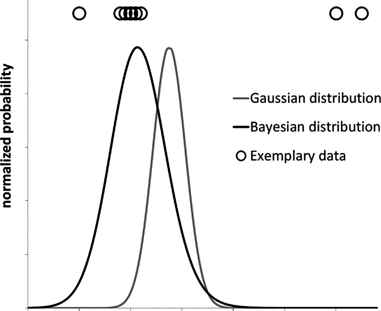
Comparison between a robust Bayesian probability distribution (Eq. (7)) and a classical Gaussian distribution for a given exemplary set of experimental data points (shown above the plotted distributions). This purely qualitative example shows that the robust Bayesian regression method suppresses apparent outliers, while the Gaussian distribution assigns equal significance to all data points.
After some mathematical operations, maximization of the posterior leads to equation (4) with the weights substituting the factors gi which are dependent on the difference Ri = Ei – Ti for each of the i’th experimental point:
| 8 |
where
| 9 |
To solve Eq. (8) an iterative procedure is required, usually readily accomplished with a simple numerical algorithm (Figure 2). As shown by Sivia and Skilling,20 if such an approach is applied to a monotonically varying curve, the outliers lose their weights and the parameter values of the curve, obtained according to the flow chart shown in Figure 2, are very close to the true ones.
Figure 2.
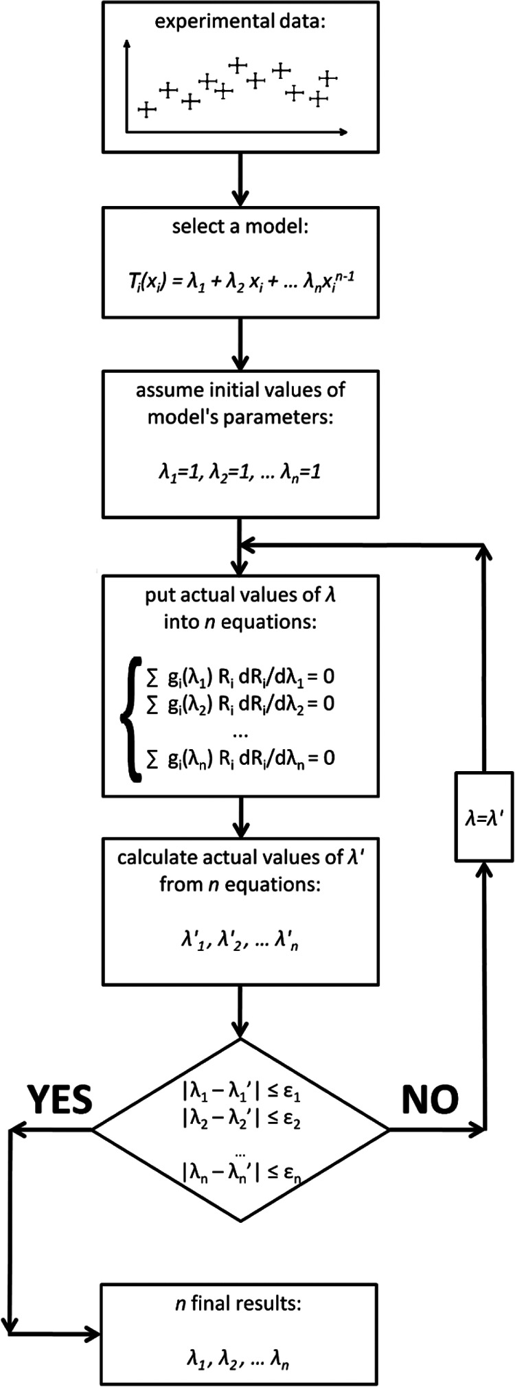
Numerical algorithm of robust Bayesian regression analysis. The parameter ε should be as low as possible, however, in practice it suffices that ε is approximately one order of magnitude smaller than the significance of λ.
Sivia and Skilling20 have also shown that a change in the prior, Eq. (5), to the so-called Jeffrey’s prior does not result in any essential change of the final conclusions. Thus, such a procedure can be used for radon analysis—where outliers are frequently found—to determine proper values of the fitted curve parameters, λ = {λ1, λ2,…, λn}, with their estimated uncertainties σλ = {σ1, σ2,…, σn}. To make this procedure effective, the number of outliers cannot exceed the number of “true” points. Otherwise, distinction between these 2 classes of points is not possible.23
Proper curve fitting is not the only advantage of the Bayesian method. Additionally, the Bayes theorem may connect the probabilities of P(T|E) ∼ P(E|T), which may then be used to estimate the relative reliability (i.e., Bayes factors) of 2 theoretical models, Ts, if the same experimental data, E are applied.25 The posterior probability (reliability) of a model T with the fitting parameter λ, using the marginalization procedure can be written20 as:
| 10 |
P(E|λ, T) corresponds to the likelihood function of a single model, represented by the Gaussian distribution around the expected value λ0 ± σλ with maximum probability of the likelihood function equal to P(E|λ0, T). The prior probability P(λ|T) can be assumed as a uniform distribution U(λmin, λmax).20 Because such form of P(λ|T) is independent of λ (within its range), the integral (10) can be approximated by .20,25 As λ0 corresponds to the parameter found by the robust Bayesian best fit method for model (curve) T (Figure 2), the maximum value of the likelihood function P(E|λ0, T) can be replaced by the set of Pi given by Eq. (7) and the final form of the reliability function can be approximated21 by:
| 11 |
Equation (11) corresponds, however, to the case where model T has only one (n = 1) fitting parameter, λ0 ± σλ. In the case of fitting n model parameters λ = {λ1, λ2,…, λn} with their estimated uncertainties σλ = {σ1, σ2,…, σn}, the most general form of Eq. (11) can be presented21,25 as:
| 12 |
Here n represents the number of experimental points (xi, Ei) with “vertical” uncertainties σ0i each, to which model T is fitted using n fitted parameters λ ± σλ. The selection of values of λmin and λmax, for all λs is however quite difficult. In the simplest case they may be taken as the smallest/largest possible values of the considered parameter λ using the highest span that can be tolerated by the data.
In the final step of this analysis the Bayes factor is calculated for the 2 models, say A and B, to test which of them is more likely to describe the data:
| 13 |
where probabilities in Eq. (13) are composed of posterior probabilities of models including their respective prior probabilities. If WT is greater than 1, model A wins over B. If WT ≈1, both models have the same credibility.21,25 This approach was applied in our earlier meta-analyses of radon data.17,21,22
Randomized (Monte Carlo) Data Binning
In many epidemiological studies, especially in the so-called pooled-studies and meta-analyses, several hundred or even several thousand data points representing lung cancer risk against radon concentration need to be analyzed. Many issues arise when analyzing such large numbers of data points, such as simply their readability or selection of suitable methods of handling their statistical fluctuations. Most authors merge several data points into a single value. This results in a reduced number of bins or classes which, in the opinion of authors who undertake such reduction, are much easier to read and more practical in further data analysis, as far fewer merged data points then need to be handled.3,9 By merging many data points into single point values, one may apparently reduce their uncertainty and considerably facilitate their analysis. However, any claim that such aggregation is more practical is erroneous, because every binning selection invariably leads to loss of information.
Such a data merging process is illustrated in Figure 3, where Figure 3A presents the original data of an ecological study of the relative risk of lung cancer related to low radon concentrations in Poland.26 The same data are presented in Figure 3B, but now reduced to 4 points only by applying arbitrarily selected binning ranges. The mean values of the slopes are different, however, without any statistical significance.
Figure 3.

Ecological data on the relative risk [%] of lung and bronchus cancers, versus low concentrations [Bq/m3] of radon in Poland26: (A) original data, (B) data merged to 4 points after arbitrarily selected binning (bin ranges: 0-33, 33-45, 45-70 and above 70 Bq/m3). The slopes, a, of the linear (1+ax) fits are (−0.177 ± 0.134) [Bq− 1 m3] and (−0.260 ± 0.141) [Bq− 1 m3] for plots (A) and (B), respectively. All uncertainties (both vertical and horizontal) represent one standard deviation.
In data analysis, data binning may be tempting, but may also raise questions, not only connected simply with information loss. For example, in the case of larg HueD_Ref3 e scatter of data points, as generally observed in many radon studies, merging data inevitably raises questions as to the manner according to which data are binned: ranges of bins (ranges of radon concentrations or doses to lungs) need to defined and justified. Otherwise, any bin selection may be considered to be subjective and arbitrary.
Proper binning is of crucial importance if a model (function) is to be fitted to such merged data points, because it opens the gate to data manipulation. For example, in a recent paper,22 we demonstrated the case of establishing best linear fits to data originally described in the meta-analysis by Dobrzyński et al,17 using 2 different data binning selections. This clearly demonstrates the importance of proper binning: after one choice of binning a linear increase is favored, while after a different bin selection, favored is a linear decrease (Figure 4). Note that in both cases, the same original 32 case-control data underwent analysis—the only difference being in bin selection.
Figure 4.

A re-analysis of 32 case-control data points listed by Dobrzyński et al,17 excluding ecological data, after merging groups of experimental points into single values within bins under arbitrarily defined boundaries: (A) bin ranges (Bq/m3): 0-37, 37-50, 50-75, 75-125, 125-175, 175-270 and 270-800, resulting in a positive slope fit (“pro-LNT” conclusion); (B) bin ranges (Bq/m3) 0-37, 37-53.5, 53.5-65, 65-100, 100-124, 124-150.1, 150.1-200, 200-600 and 600-800, resulting in a negative slope fit (“pro-hormetic” conclusion). In both cases, the same input data were used.22
Figure 4A and B present the best linear (2-parametric) fits using the classic least squares method.22 One should note that the difference between values of the slopes of these 2 fitted lines is not statistically significant—thus supporting the general conclusion drawn by Dobrzyński et al17— irrespective of the manner of bin selection. Nevertheless, depending on the choice of binning strategy, widely differing conclusions may be drawn, despite their weak statistical significance.
The example presented in Figure 4 clearly shows that binning selection may lead, even unintentionally, to misinterpretation of data—2 completely different conclusions may be drawn from analysis of the same data set. Therefore, the simplest solution is to avoid data binning and to fit the model to the full set of original data. However, as mentioned above, this may not be possible or be impractical for other reasons. Therefore, the choice of proper binning needs to be justified by verification of the sensitivity of the final result on bin selection.
The most objective and appropriate way is then to analyze every possible ordinary binning and to verify which bin selection is most representative. However, with sets containing hundreds of data points, the only way to analyze such data is by numerical randomization, e.g. by applying Monte Carlo techniques.
The proposed methodology is quite simple and consists of a few numerical steps, as illustrated by the flowchart in Figure 5:
Figure 5.
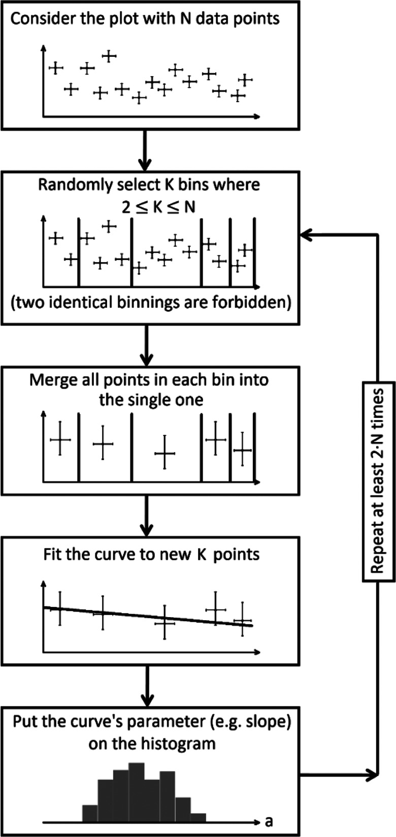
Algorithm of the random binning procedure which delivers a histogram of fitted parameters and their distribution.
select a random number of bins, which should be less than the number of data points;
select at random the borders (ranges) of bins (verifying that this selection of bins has not been made earlier);
gather data points within each bin into a single point value with its proper uncertainty (inverse-variance weighting);
use Orthogonal Distance Regression to fit the same appropriate model (curve) to the new set of binned data points, after merging points in all bins;
plot the fitted parameters (e.g., in the form of a histogram of slopes, in the case of a linear fit);
repeat all above steps, ensuring that every possible binning was analyzed, within the available computing power.
The Maximum Entropy Method
Lung cancer may be caused not only by radon alone, but also by many other factors, acting independently or synergistically with radon. Thus, in the interpretation of lung cancer versus radon concentration epidemiology data, confounding factors should be taken into account. Simeonov and Himmelstein27 estimated the relative strengths of various correlations between lung cancer and factors other than radon, indicating the presence of a strong correlation between radon concentration, altitude at which inhabitants lived, and the level of UVB.27 It is clear that within a sufficiently narrow range of altitudes, any correlation with radon concentration should be weak. One could then undertake an analysis of lung cancer versus radon concentration over such a limited height region. However, if such an analysis were to be carried out, the number of “experimental” points should be sufficient to achieve a reliable result. In a similar fashion, one could limit the ranges of other parameters (elevation and/or level of UVB) in a thus stratified analysis of lung cancer versus radon concentration.
Although the above methodology, employed in our recent paper,22 appears to be simple, in reality one has to consider the scatter of points with respect to their claimed accuracy, which may lead to questionable final results. Therefore, we decided to use the Maximum Entropy Method (which is also, as described, a Bayesian method20) to analyze cancer probability against 2 simultaneous parameters, i. e. radon concentration and altitude, or radon concentration and level (intensity) of UVB. Here, we first made an attempt to verify whether the correlation of lung cancer with the level of UVB (irrespectively of altitude) and radon concentration, given in the paper by Simeonov and Himmelstein,27 is—or is not—essential to contract lung cancer. We first performed this verification in a manner described earlier.22 In our second step, we also took the inaccuracy of the input data into account. Full details of this non-standard procedure are given in the following paragraph.
Maximum entropy approximation procedure
Approximation algorithms, commonly applied in data analysis, are usually based on minimization of some metric value (e.g., least-squares) with respect to the coefficients of an a priori assumed function. Being very useful in most cases, this approach however fails if no trivial form of the approximating distribution is known. Moreover, any assumption of a specified analytical form of this approximating distribution function introduces some bias and may lead to non-physical artifacts.
The Maximum Entropy Method used here, is free from such drawbacks. Having the set of nodal points {r i} (in D-dimensional space) in which the measured values of the function are equal to {fi}, approximation at point r within the convex hull (ConvH) span by the nodes {r i} may be defined via the transformation:
| 14 |
The functions si(r), for a given vector r, assume the role of weights for fi values and are called shape functions. Reproducing the reasoning of Arroyo and Ortiz,28 si(r) functions are chosen to be positive and to maximize the information entropy:
| 15 |
A normalization condition must also be observed:
| 16 |
as well as the so-called first consistency condition:
| 17 |
which is introduced to reproduce affine functions. The 2 forms of Eq. (16) are equivalent as long as the shape functions form a normalized base. It should also be apparent that the value of this shape function at any given point r becomes its expected/expectation value. Taking these 2 additional constraints into account, one may seek the maximum of the Lagrange function:
| 18 |
In general, the dimension of the λ 2 vector is equal to the dimension of r. The shape function si maximizing the above functional, given in exponential form, is:
| 19 |
with being the partition function. It can be shown that the vector of Lagrange’s multipliers should be chosen in such a way that the free energy for each point r is minimized independently:
| 20 |
Minimization of the functional given by Eq. (20) is equivalent to fulfilment of the first consistency condition. However, from the technical point of view, numerical minimization is usually easier than numerical solution of a set of nonlinear equations.
Having obtained the vector λ 2, one can find the shape functions si and, finally, approximate the value of the distribution g(r).
The above-described procedure applies to a uniform prior distribution of the shape functions. This allows the obtained distribution g(r) to be the flattest possible (according to the maximum entropy principle). However, in some cases, if Gaussian prior shape functions are chosen with arbitrary widths, β, centered at a given nodal point, then29:
| 21 |
Although β can be treated as the next parameter of minimization, in most cases it is fixed. Tuning this multiplier allows one to better reproduce the experimental intensities, given by the set {fi}, simultaneously eliminating experimental noise. In this approach β is not universal, but depends on the uncertainty σi of the i-th intensity fi and the point spacing (Δx; Δy): , where Δx and Δy denote the components of ri-r. One may observe that points with relatively small experimental error are incorporated within the peaked Gaussian form, while very uncertain points are “smeared-out” over many neighbors.
Results
Randomized Data Binning
To verify the above-presented method of randomized (Monte Carlo) data binning, this approach was applied to the 32 case-control and 2 ecological studies presented and re-analyzed in the paper by Dobrzyński et al.17 In this case, a linear fit with a fixed Y axis intersection, i.e. the function RR = 1 + a·D, was used, and every slope parameter (a value) obtained was plotted in the form of a histogram. This histogram (Figure 6) demonstrates that in practice only negative trends (a < 0) are possible, displaying a maximum at about −0.00037. This is yet another demonstration of the need for caution when selecting data bins, as the choice of binning may bear upon the final conclusion of such an analysis. Note that the above-described method not only shows which value (here, of the slope parameter) appears most frequently, but also what is its most likely distribution.
Figure 6.
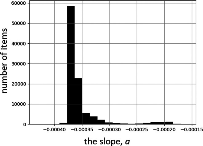
Histogram of slope values of linear fits (RR = 1 + a·D) to data of the 34-study meta-analysis by Dobrzyński et al.17 100,000 Monte Carlo iterations of randomly selected binning (cf. Figure 5) were performed.
Following a similar analysis of the case presented in Figure 3A, the resulting distribution of slope parameters is represented by the histogram in Figure 7. In this case, however, 3 possible general trends occur, all with negative slope values.
Figure 7.
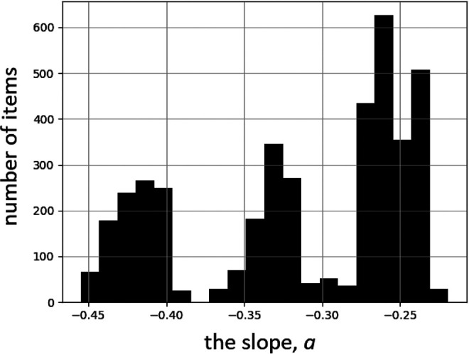
Histogram of slope values of linear fits (RR = 100% + a·D) to data of the ecological Polish study,26 cf. Figure 3A. 2000 Monte Carlo iterations of randomly selected binning (cf. Figure 5) were performed.
Maximum Entropy Method
In our last paper (Reszczyńska et al)22 the isocontours of lung cancer morbidity in the plane altitude-radon concentration, calculated for all UVB regions, were displayed for low, medium and heavy smoking prevalence. In Figure 8 we show similar isocontours (maps) in the plane UVB level—radon concentration, calculated for all altitudes and all inhabitants. In all these cases, the accuracy of “experimental” points was not taken into account. Maps for low smoking prevalence are not shown because too few data points were available to carry out a reasonable 3-dimensional analysis.
Figure 8.

Maps of lung cancer morbidity versus UVB level (in kJ/m3): (A) radon concentration plane for the whole analyzed population, (B) medium smoking prevalence, (C) high smoking prevalence. All altitudes have been taken into account. The color bar below every figure shows the morbidity of lung cancer per 100,000 inhabitants. The Maximum Entropy Method with its Eq. (19) was used.
It was shown (Reszczyńska et al)22 that at any altitude at which people live, one observes a decrease of lung cancer morbidity with increasing radon concentration. This is definitely a new and important piece of information, contradicting the conclusion of Simeonov and Himmelstein.27 The apparent maximum of morbidity at UVB levels of about 1000-1100 kJ/m3 is puzzling. This effect was neither shown nor discussed by Simeonov and Himmelstein.27
In what follows, we show results obtained with the same algorithm as that used earlier (Reszczyńska et al)22—therefore called the “Original maxEnt.”
Figure 9 displays maps of the distribution of lung cancers, versus elevation and radon concentration. Were correlation between the intensity of UVB and the altitude full, Figures 8 and 9 should bear the same information. However, the datasets in both cases are slightly different, so presentation of both figures seems appropriate. In addition, in Figure 9 the location of “experimental” points is shown. Taking into account their density distribution, one may appreciate the strength of the Maximum Entropy Method in the reconstruction of 3D maps.
Figure 9.

Distribution of lung cancers, versus elevation and radon concentration, for men and women taken together. (A) Low smoking prevalence, (B) medium smoking prevalence, and (C) high smoking prevalence. Dots in these plots represent the positions of points, as given in the catalog of Simeonov and Himmelstein.27 Elevation is in kilometers. “Original MaxEnt” represents Eq. (19).
If uncertainties of the data, Eq. (21), are taken into account, following the above-presented procedure, one obtains maps shown in Figure 10.
Figure 10.

Distribution of lung cancers, versus elevation and radon concentration with uncertainties taken into account and (▵x, ▵y) = (5.0, 0.06). The order and description of maps is the same as that in Figure 9. The only difference is in the use of Eq. (21) in the reconstruction.
Clearly, larger differences are seen in maps related to low smoking prevalence. This is due to the limited number of data points. Therefore, in what follows, these data are not included. Nor should one treat data points close to the border lines as being meaningful.
As mentioned earlier, accounting for data uncertainties is not trivial. The only solid information available is the relative number of lung cancers, for which it is possible to calculate uncertainties in the manner shown earlier (Reszczyńska et al).22 In fact, such an analysis, using Eq. (8), was carried out for the following set of (Δx; Δy) (in Bq/m3 and km, respectively): {(2.25; 0.03), (2.25; 0.06), (5.0; 0.03), (5.0; 0.06)}. Such a multitude of reconstructions allows one to verify the sensitivity of the major features of the reconstructed maps on the selected parameters.
In the case of high and medium smoking prevalence, one may infer from Figures 9 and 10 that incorporation of uncertainties does not substantially distort these maps. In particular, the maps distinctly show that the number of lung cancers decreases with elevation, while for any elevation a decrease of lung cancers with radon concentration is observed. This conclusion is supported by independent analysis of the data for men and women, cf. Figure 11.
Figure 11.

Distribution of lung cancers versus elevation and radon concentration for men in regions with medium (A) and high (B) smoking prevalence. (C) and (D) Show distributions for women, using the same convention as that for men. Elevation is in kilometers.
As seen in Figure 11, in the case of men alone our conclusions are the same as for those where results for men and women together are displayed. However, the maps for women, especially living in areas with high prevalence of smoking, are quite different from those for men: a decrease of lung cancers with radon concentration is seen, however less evident if altitude is also considered.
On the Distribution of Radon Concentration
In order to proceed further with data analysis, we verified the distribution of radon concentration at any altitude. One may expect it to follow a log-normal distribution, due to several factors affecting radon accumulation inside and outside the inhabitant’s dwelling. Regional distributions must represent the sum of a multitude of local distributions, and, according to the British Health Protection Agency, local distributions should also be represented by log-normal distributions. Simeonov and Himmelstein27 have verified that this is indeed the case for indoor radon concentrations, within the Lawrence Berkeley National Laboratory High-Radon Project. The distribution they obtained is presented in Figure 12. It acquires the form of a Gaussian distribution if plotted versus logarithm of radon concentration. Thus, one may state that the observed distribution is close to log-normal. Within the framework of our data analysis, any deviations from the assumption of a log-normal distribution of radon concentration are not expected to seriously affect our conclusions.
Figure 12.
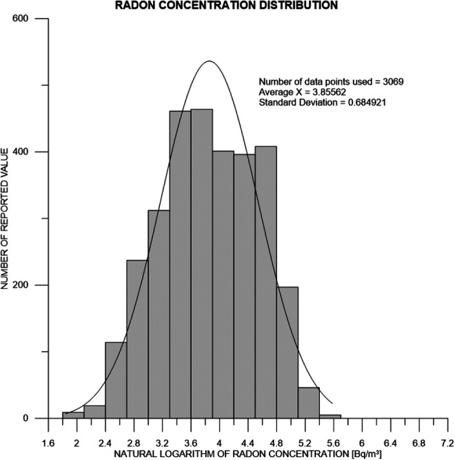
Log-normal distribution of radon concentration at any altitude.27 The fitted Gaussian shows that the median concentration of naturally occurring radon is 47.3 Bq/m3 within 68% CI (23.8-93.7 Bq/m3) and 95% CI (12.0-185.9 Bq/m3).
One should note that relative uncertainty values in the measured radon concentrations, proportionately larger at lower radon concentration ranges, may affect the shape of the plotted distribution.
There are several reasons for the difficulty in estimating the uncertainty of radon concentration. From the result given in Figure 12 in terms of the logarithm of radon concentration, estimation of any median, with 68% CI (confidence intervals), will result in a median value ranging between 0.5 to 2.0 times the original (linear) value. To improve on this rather crude approach, one could perhaps use the Bayesian approximation, as described, e.g. by Price et al.30 However, due to the asymmetrical nature of the resulting linear uncertainties, if linear regression is carried out without taking these asymmetric ranges of uncertainties into account, the resulting slope of the regression-fitted line will not be fitted correctly.
Discussion
Our analysis, which dealt mainly with ecological data on lung cancer incidence in the US, provided by Simeonov and Himmelstein,27 has not been principally addressed at precisely establishing radon-induced risks of lung cancer incidence or mortality. Rather, our focus was on refining methodological approaches to extracting as much information as possible from the available data and to drawing the most likely rational conclusions, in view of the presence of confounding factors. The ecological data set gathered by Simeonov and Himmelstein27 is the best available and presents the global aspects of lung cancer over the territory of US, irrespective of individual fates or their detailed cases. While the uncertainties in the number of lung cancers may be readily calculated basing on the number of inhabitants over given regions or areas,22 accounting for the effect of confounding factors, especially smoking, on the uncertainty of the final result is much more complex. Simeonov and Himmelstein27 suggested 3 main factors to be strongly correlated with lung cancer, namely radon concentration, altitudes where people live, and to a lesser extent, the level of UVB. Generally, the dose of ionizing radiation goes up as a function of elevation as well as UVB. Additionally, in their data, smoking prevalence has been classified only within 1 of 3 categories: high, medium or low. In our previous study (Reszczyńska et al),22 we generally followed their classifications with some slight modification. By applying, presumably for the first time, the Maximum Entropy Method to the data of Simeonov and Himmelstein,27 we found a decrease of lung cancer morbidity with increasing radon concentration at any altitude of inhabitation. This is definitely a new and important piece of information which contradicts their conclusions. This method also yielded an apparent maximum of morbidity at UVB levels of about 1000-1100 kJ/m3, a puzzling result, neither shown nor discussed by these authors. It should be noted that the Maximum Entropy Method treats all parameters as being independent—no correlation of these parameters is assumed in the algorithm.
Undoubtedly, interpretation of ecological data is not easy. In particular, the problem of confounding factors is very difficult to handle, casting serious concerns as to the reliability of the resulting dose-effect dependences. A classic example is the fate of the well-known ecological work of Cohen.12 By examining the correlation between cancer mortality and radon concentration within over 1700 counties in US, Cohen demonstrated that lung cancer mortality clearly decreases with increasing environmental radon concentration—a conclusion which dramatically challenged the widely accepted LNT (Linear-No Threshold) paradigm.12 In response to criticism of his work,31,32 Cohen submitted an elaborate mathematical analysis accounting for up to 50 confounding factors and confirming the general conclusions of his original paper. On the other hand, certain inherent limitations of such ecological analyses should be noted. For example, in the context of Cohen’s analysis, Puskin32 found negative correlations between radon concentration and county-level rates for smoking-related cancers other than radon. Nevertheless, expert bodies, including UNSCEAR,16 decided to side with Cohen’s critics, in effect completely ignoring the results of Cohen’s analysis. The case studies of Thompson et al,11,33 Becker,13,34 Bogen,35,36 Krstić37 or Sanders,38 and the more recent studies of Cuttler39 or of the University of Oslo biophysical group40 have not changed this situation either, as may be inferred, e.g. from a recent paper by Malinovsky et al.9 One has to bear in mind that in all studies discussed so far, the set of confounding factors was more or less the same. Nilsson and Tong41 extensively discuss the well-known results of Darby et al3 and of Krewski et al,42 cited by many researchers and also by UNSCEAR,16 to show that the general acceptance of risk of lung cancer morbidity increasing with radon concentration even at low doses, may be flawed, as many confounding factors have so far not been considered. Among those factors, there is general consensus that the main cause of lung cancer is smoking. However, especially in uranium miners subjected to high radon doses,15 strong correlation with radon concentration was observed—namely, exposure to radon together with cigarette smoking, significantly increased their cancer rate,. It is intriguing that inclusion of smoking as a confounding factor did not make Cohen’s12 conclusions qualitatively different. In turn, Krstić37 in Figure 2 of his paper showed by performing linear regression of WHO43 and OECD44 data, that for non-smokers, lung cancers decrease with increasing radon concentration. In his work, Krstić37 also pointed to other relevant confounding factors, such as proper diet, environmental tobacco smoke, asbestos or arsenic in drinking water.
The correlation we suggest between lung cancers and UVB intensity should be confronted with data published by Boscoe and Schymura.45 In their work, values of UVB intensity of were acquired from aerial (satellite) measurements and frequencies of many different types of cancer were considered, however lung cancers were not included. Thus, one may concur with Simeonov and Himmelstein27 that UVB intensity could appear as a predictor of lung cancer merely due to its correlation with e.g. altitude, thus supporting the conclusion of Hayes.46 However, what we show here is a more general view, namely that a negative correlation between lung cancers and elevation is observed at any UVB level. As shown in Figure 8, at any given UVB intensity (or height), lung cancer frequency tends to decrease with increasing radon concentration.
Our application of Bayesian approaches, with respect to linear regression and to the application of the Bayes factors of proposed hypotheses, applied to the data of Simeonov and Himmelstein27 has followed our earlier work and is discussed in more detail elsewhere.22 Here we can only stress once again that, due to the large scatter of data points, the uncertainties of the values of parameters, such as the slopes of the best-fitted straight lines may be larger than those estimated from pure statistics. In fact, many slope values of straight lines may be fitted to such data equally well. Following Bayesian logic, most likely is the simplest hypothesis—namely that no effect of radon concentration on cancer occurrence is observed over the radon concentrations covered by these data. This is generally consistent with our earlier findings17,21 where the Bayesian statistics approach was used for radon data analysis for the first time. The trend we actually observed and which also follows from the present paper, namely a decrease of lung cancer morbidity with radon concentration, may be confirmed or disproved only if better methods of handling the present data are elaborated—or if new surveys, better accounting for the various confounding factors (especially for smoking patterns) are carried out.
We believe to have convincingly shown the importance of proper data binning and the evident effect of binning on the interpretation of the final results. We discussed at length the possible consequences of binning data, with respect to selection of intervals of radon concentrations over which the number of lung cancers is measured and averaged within the chosen bin interval. Indeed, binning is often justified as being a more practical aggregation of data points. This is definitely misleading, since the apparent simplicity of compressing individual values to frequencies of (coarser) intervals inevitably leads to loss of information and introduces a definite bias. In fact, such binning cannot reduce the uncertainty of model selection. It is intuitively quite clear (and can be strictly proven on theoretical grounds) that the binned data (and analyses based on such data) are inferior to those based on original non-aggregated data. Modern statistical approaches should aim at quantifying such loss of information and at accounting for such loss within any data analysis undertaken. This is not merely a theoretical consideration—information contained within a bin can be extremely useful in initial model selection (testing of hypotheses) and in assessing whether the model may adequately represent the data set (lack of acceptable fit may then be signalled, even if a perfect fit to the binned data points is achieved). Data point binning and the consequences of their aggregation are complex issues which involve not only the introduction of unspecified biases but also introduce more subtle distributional features, leading to changes in variability in both directions—potentially leading to either false positive or false negative results of testing hypotheses. Therefore, we have proposed a computationally straightforward method which may potentially demonstrate whether the tested binning could generate false conclusions. We also pointed to the difficulty of proving that any particular choice of binning intervals may be optimal, proposing instead either no binning, or, if this is impractical, randomized bin selection using the Monte Carlo technique, to indicate the most frequent (or likely) outcome. In this manner, it is possible to seek the dominating trends in the slopes of the resulting best-fitted lines (models). In one example of our analysis of combined case-control and ecological data, practically all randomly selected bin configurations yielded a distinct negative slope value trend, as shown in Figure 6, lending strong statistical support for such a conclusion. On the other hand, several trends in slope value (local maxima) may occur as a result of randomized binning, such as in the case of the Polish ecological study (Figure 7), indicating no single preference in the random binning process. However, since all 3 slope value trends in that figure are negative, at least the negative sign of the slope of the model line is established well enough. To summarize, stringent analysis of the binning process and its correct and objective selection appear to be of crucial importance in objective data analysis. To illustrate this point, Malinovsky et al,9 having reduced all their data into 4 bins only, calculated their weighted median values of ORs (Odds ratios), obtaining an OR of 1.35 with impressive credibility (P < 0.0001) for their highest median radon concentration of 283 Bq/m3. In our recent paper (Reszczyńska et al)22 we contested their work and their conclusions. Indeed, as pointed out by Scott,18,47,48 if one considers the variability of natural background measurements, an OR value of 1.35 may not be realistic, which supports our view. Much higher Nor may radon concentrations of the order of 10 kBq/m3, considered by Malinovsky et al,9 may be detrimental to human health, but, as evidenced by the well-being of inhabitants of radon-rich areas, this is not always the case in areas where radon concentrations up to 31 kBq/m3 have been consistently measured.49-51 However, at high radon concentrations (>1000 Bq/m3), practically all case-control and epidemiological studies support its detrimental effect to human health.10,16
We have presented in considerable detail the Maximum Entropy Method as applied to handling confounding factors in radon data analysis, such as simultaneous analysis of 2 (i.e., lung cancer versus radon concentration and altitude) or more factors (i.e., additionally, against smoking prevalence). This method was very likely used for the first time in the analysis of radon epidemiology data. The Maximum Entropy Method not only replaces typical multi-parameter analysis where the effect of confounding factors is described by linear dependences, but also allows more complex relationships to be considered. In fact, our development of this novel approach was stimulated by the view of Simeonov and Himmelstein27 that the negative correlation between lung cancers and concentration of radon is due to the strong dependence of lung cancers on the altitude of inhabitants—as based on their linear multi-parameter analysis. By applying our Maximum Entropy analysis to their data set, we reconfirmed our earlier statement that lung cancer morbidity decreases with altitude, and that at any altitude lung cancer morbidity systematically decreases with increasing radon concentration. Unfortunately, lack of sufficient detail on smoking prevalence in the data set of Simeonov and Himmelstein,27 precluded any more detailed Maximum Entropy analysis of smoking as a confounding factor. While grouping of the smoking prevalence in their data only into 3 (high, medium or low prevalence) categories limited our analysis, we did not observe any significant difference between the effects of high or medium smoking habits. We were also able to show that women are less susceptible to smoking-related lung cancer than men (Figure 11). It is unfortunate that this data set does not permit a more definitive analysis of the dependence of lung cancer morbidity on smoking—with or without radon—to be performed. In summary, we contest the opinion of Simeonov and Himmelstein27 that any decrease of lung cancer occurrence with increasing radon concentration is merely due to the correlation between all 3 confounding parameters considered. In fact, it is known that the level of radon concentration increases with increasing altitude.52 Thus, radon concentration is the leading factor in the analysis of lung cancer morbidity. Our results demonstrate that the Maximum Entropy Method, as applied to the available epidemiology data, rationally weighs over the scattered data and provides us with results more meaningful than those delivered by the classical least-squares method, or even by both Bayesian approaches.
Our interest in studying the risk of cancer at residential radon concentrations below about 200 Bq/m3, corresponding to annual effective doses of some 5 mSv or less, or due to radon-induced doses received by radon spa visitors (presumably for curative purposes53), inevitably leads us to the issue of linear extrapolation from higher radon concentrations, i.e. to the Linear-no Threshold (LNT) hypothesis, versus other models (threshold or hormesis). Our consistently observed decrease of lung cancer morbidity with increasing radon concentration, albeit not statistically significant, supports the findings of Cohen12 and concurs with the recent work of Pennington and Siegel54 who support the threshold model against the scientifically unfounded LNT. In their 2015 paper, Cuttler and Sanders55 postulate that the threshold for radon-induced lung cancer may be as high as 2100 Bq/m3—an order of magnitude higher than the 200 Bq/m3 range considered here. The threshold model in the more general case of radiation-induced cancer is also strongly supported by Pennington and Siegel.54 Moreover, the Schneeberg study by Martin,56 also discussed by Henriksen40 concerns radon concentrations as high as 1000 Bq/m3 and indicates no adverse effects, which would lend support to the threshold model.
Conclusions
Residential radon data from US registries27 were analyzed using various methods with particular emphasis on the Maximum Entropy Method, applied in this work for the first time. In summary, we arrive at the following conclusions:
Binning of original data should be carefully thought through, as it may significantly affect the final conclusions of the analysis. Randomized binning using Monte Carlo techniques may indicate the most likely trends in reaching such conclusions. An example of the possible outcomes of such data binning were presented for the Polish radon ecological study.26
The immanent scatter of residential radon data requires that more advanced statistical tools be applied, such as the robust Bayesian regression method with model selection, or the Maximum Entropy Method. Our 3-parameter analysis by the Maximum Entropy Methods shows that an increased concentration of radon (at least up to about 200 Bq/m3) does result in lowering lung cancer risk irrespectively of altitude (up to 3000 m above sea level) and of UVB intensity. This qualitatively supports the results of Cohen.12
The highest incidence of lung cancers is found over areas at which the UVB level is close to 1000 kJ/m3, and the level of radon concentration is relatively low.
On application of more advanced statistical tools in the analysis of radon data, the widely postulated and legally enforced linear no-threshold (LNT) increase of lung cancer risk with radon concentrations up to several hundred Bq/m3, is not supported by the presented analysis of officially approved and distributed data.
Footnotes
Declaration of Conflicting Interests: The author(s) declared no potential conflicts of interest with respect to the research, authorship, and/or publication of this article.
Funding: The author(s) received no financial support for the research, authorship, and/or publication of this article.
References
- 1. Council Directive 2013/59/Euratom of 5 December 2013. Laying down basic safety standards for protection against the dangers arising from exposure to ionising radiation. Published 2013. Accessed March 1, 2021. https://eur-lex.europa.eu/eli/dir/2013/59/oj
- 2. Vogeltanz-Holm N, Schwartz GG. Radon and lung cancer: what does the public really know? J Environ Radioact. 2018;192:26–31. [DOI] [PubMed] [Google Scholar]
- 3. Darby S, Hill D, Auvinen A, et al. Radon in homes and risk of lung cancer: collaborative analysis of individual data from 13 European case-control studies. BMJ. 2005;330(7485):223–226. [DOI] [PMC free article] [PubMed] [Google Scholar]
- 4. Rodríguez-Martínez Á, Torres-Durán M, Barros-Dios JM, Ruano-Ravina A. Residential radon and small cell lung cancer. A systematic review. Cancer Lett. 2018;426:57–62. doi:10.1016/j.canlet.2018.04.003 [DOI] [PubMed] [Google Scholar]
- 5. Dempsey S, Lyons S, Nolan A. High radon areas and lung cancer prevalence: evidence from Ireland. J Environ Radioact. 2018;182:12–19. [DOI] [PubMed] [Google Scholar]
- 6. López-Abente GNúúez O, Fernández-Navarro P, Barros-Dios JM, et al. Residential radon and cancer mortality in Galicia, Spain. Sci Total Environ. 2018;610:1125–1132. [DOI] [PubMed] [Google Scholar]
- 7. Veloso B, Nogueira JR, Cardoso MF. Lung cancer and indoor radon exposure in the north of Portugal—an ecological study. Cancer Epidemiol. 2012;36(1):e26–e32. [DOI] [PubMed] [Google Scholar]
- 8. Elío JA, Crowley Q, Scanlon R, Hodgson J, Zgaga L. Estimation of residential radon exposure and definition of radon priority. Environ Int. 2018;114:69–76. [DOI] [PubMed] [Google Scholar]
- 9. Malinovsky G, Yarmoshenko I, Vasilyev A. Meta-analysis of case–control studies on the relationship between lung cancer and indoor radon exposure. Radiat Environ Biophys. 2019;58(1):39–47. Epub Dec 8, 2018. [DOI] [PubMed] [Google Scholar]
- 10. Effects of Exposure to Radon (BEIR VI). Committee on Health Risks of Exposure to Radon, Board on Radiation Effects Research, Commission on Life Sciences, National Research Council. National Academy Press; 1999. [Google Scholar]
- 11. Thompson RE, Nelson DF, Popkin JH, Popkin Z. Case-control study of lung cancer risk from residential radon exposure in Worcester County, Massachussetts. Health Phys. 2008;94(3):228–241. [DOI] [PubMed] [Google Scholar]
- 12. Cohen BL. Test of the linear no-threshold theory of radiation carcinogenesis for inhaled radon decay products. Health Phys. 1995;68(2):157–174. [DOI] [PubMed] [Google Scholar]
- 13. Becker K. Health effects of high radon environments in central Europe: another test for the LNT hypothesis. Nonlinear Biol Toxicol Med. 2005;1(1):3–35. [DOI] [PMC free article] [PubMed] [Google Scholar]
- 14. Deetjen P. Biological and therapeutical properties of radon. In: Katase A, Shimo M, eds. Radon and Thoron in the Human Environment. World Scientific; 1998:515–522. [Google Scholar]
- 15. Zarnke AM, Tharmalingam S, Borenham DR, Brooks AL. BEIR VI radon: the rest of the story. Chem Biol Interact. 2019;301:81–87. [DOI] [PubMed] [Google Scholar]
- 16. UNSCEAR 2006 Report, Annex E. Sources-to-Effects for Radon in Homes and Workplaces. United Nation; 2009. [Google Scholar]
- 17. Dobrzyński L, Fornalski KW, Reszczyńska J. Meta-analysis of thirty two case-control and two ecological radon studies of lung cancer. J Radiat Res. 2018;59(2):149–163. [DOI] [PMC free article] [PubMed] [Google Scholar]
- 18. Scott BR. Epidemiologic studies cannot reveal the true shape of the dose-response relationship for radon-induced lung cancer. Dose-Response. 2019;17(1). [DOI] [PMC free article] [PubMed] [Google Scholar]
- 19. Fornalski KW, Adams R, Allison W, et al. The assumption of radon-induced cancer risk. Cancer Causes Control. 2015;26(10):1517–1518. [DOI] [PubMed] [Google Scholar]
- 20. Sivia DS, Skilling J. Data Analysis: A Bayesian Tutorial (Second Edition). Oxford University Press. 2006. [Google Scholar]
- 21. Fornalski KW, Dobrzyński L. Pooled Bayesian analysis of twenty-eight studies on radon induced lung cancers. Health Phys. 2011;101(3):265–273. [DOI] [PubMed] [Google Scholar]
- 22. Reszczyńska J, Pylak M, Fornalski KW, Mortazavi SJ, Dobrzyński L. Methodological problems in epidemiological data: the case of correlation between radon level and lung cancer. Int J Low Radiat. 2020;11(3/4):207–226. [Google Scholar]
- 23. Fornalski KW, Parzych G, Pylak M, Satuła D, Dobrzyński L. Application of Bayesian reasoning and the maximum entropy method to some reconstruction problems. Acta Physica Polonica A. 2010;117(6):892–899. [Google Scholar]
- 24. Rousseeuw P, Leroy AM. Robust Regression and Outlier Detection. Wiley; 1987. [Google Scholar]
- 25. Fornalski KW, Dobrzyński L. The robust Bayesian approach to the model selection algorithm. JSMS. 2015;1(1):8–12. [Google Scholar]
- 26. Szołucha MM, Fornalski KW. The cancer mortality and incident studies due to the natural background radiation in Poland. Int J Low Radiat. 2018;11(1):1–22. [Google Scholar]
- 27. Simeonov KP, Himmelstein DS. Lung cancer incidence decreases with elevation: evidence for oxygen as an inhaled carcinogen. Peer J. 2015;3:e705. doi:10.7717/peerj.705 [DOI] [PMC free article] [PubMed] [Google Scholar]
- 28. Arroyo M, Ortiz M. Local maximum-entropy approximation schemes: a seamless bridge between finite elements and meshfree methods. Int J Numer Meth Eng. 2006;(65):2167–2202. [Google Scholar]
- 29. Kumar S, Danas K, Kochamnn DM. Enhanced local maximum-entropy. Com Meth Appl Mech Engng. 2019;344:858–888. [Google Scholar]
- 30. Price PN, Nero AV, Gelman A. Bayesian Prediction of Mean Indoor Radon Concentrations for Minnesota Counties. University of California; LBL-35818 UC-402. Published 2005. https://escholarship.org/uc/item/41m4089f [DOI] [PubMed] [Google Scholar]
- 31. Heath CW, Jr, Bond PD, Hoel DG, Meinhold CB. Residential radon exposure and lung cancer risk: commentary on Cohen’s county based study. Health Phys. 2004;87(6):647–655. [DOI] [PubMed] [Google Scholar]
- 32. Puskin JS. Smoking as a confounder in ecologic correlations of cancer mortality rates with average county radon levels. Health Phys. 2003;84(4):526–532. [DOI] [PubMed] [Google Scholar]
- 33. Thompson RE. Epidemiological evidence for possible radiation hormesis from radon exposure: a case-control study conducted in Worcester, MA. Dose Response. 2011;9(1):59–75. [DOI] [PMC free article] [PubMed] [Google Scholar]
- 34. Becker K. One century of radon therapy. Int J Low Radiat. 2004;1(3):333–357. [Google Scholar]
- 35. Bogen KT. A Cytodynamic Two-Stage Model That Predicts Radon Hormesis (Decreased, then Increased Lung-Cancer Risk vs. Exposure). Lawrence Livermore National Laboratory; 1996. Preprint UCRL-JC-123219. [Google Scholar]
- 36. Bogen KT. Mechanistic model predicts a U-shaped relation of radon exposure to lung cancer risk reflected in combined occupational and U.S. residential data. Hum Exp Toxicol. 1998;17(12):691–696. [DOI] [PubMed] [Google Scholar]
- 37. Krstić G. Radon versus other lung cancer risk factors: how accurate are the attribution estimates? J Toxicol Environ Health A. 2017;67(3):261–266. [DOI] [PubMed] [Google Scholar]
- 38. Sanders CL. Radiation Hormesis and the Linear-No-Threshold Assumption. Springer; 2017. [Google Scholar]
- 39. Cuttler JM. Application of low doses of ionizing radiation in medical therapies. Dose Response. 2020;18(1). doi:10.1177/1559325819895739 [DOI] [PMC free article] [PubMed] [Google Scholar]
- 40. Henriksen T. Biophysics Group at UiO. Radiation and Health. University of Oslo; 2015. http://www.mn.uio.no/fysikk/tjenester/kunnskap/straling/radiation-and-health-2015.pdf [Google Scholar]
- 41. Nilsson R, Tong J. Opinion on reconsideration of lung cancer risk from domestic radon exposure. J Rad Med Prote (China). 2020;1(1):48–54. [Google Scholar]
- 42. Krewski D, Lubin JH, Zielinski JM, et al. A combined analysis of North American case-control studies of residential radon and lung cancer. J Toxicol Environ Health. 2006;69(7):533–597. [DOI] [PubMed] [Google Scholar]
- 43. World Health Organisation (WHO) handbook on indoor radon: a public health perspective. Published 2009. Accessed March 1, 2021. https://www.who.int/ionizing_radiation/env/9789241547673/en/ [PubMed]
- 44. OECD (Organization for Economic Cooperation and Development). Health at a Glance 2011: OECD Indicators. OECD Publishing; 2011. doi:10.1787/health_glance-2011-en [Google Scholar]
- 45. Boscoe FP, Schymura MJ. Solar ultraviolet-B exposure and cancer incidence and mortality in the United States, 1993–2002. BMC Cancer. 2006;6:264. doi:10.1186/1471-2407-6-264 [DOI] [PMC free article] [PubMed] [Google Scholar]
- 46. Hayes DP. Cancer protection related to solar ultraviolet radiation, altitude and vitamin D. Med Hypotheses. 2010;75(4):378–382 doi:10.1016/j.mehy.2010.04.001 [DOI] [PubMed] [Google Scholar]
- 47. Scott BR. A critique of recent epidemiologic studies of cancer mortality among nuclear workers. Dose Response. 2019;16(2). [DOI] [PMC free article] [PubMed] [Google Scholar]
- 48. Scott BR. Residential radon appears to prevent lung cancer. Dose Response. 2011;9(4):444–464. [DOI] [PMC free article] [PubMed] [Google Scholar]
- 49. Sohrabi M. World high background natural radiation areas: need to protect public from radiation exposure. Radiation Meas. 2013;50:166–171. [Google Scholar]
- 50. Mortazavi SMJ, Doss M. Comments on high radon areas and lung cancer prevalence: evidence from Ireland. J Environ Radioact. 2018;192:709–710. doi:10.1016/j.envrad.2018.03.007 [DOI] [PubMed] [Google Scholar]
- 51. Dobrzyński L, Fornalski KW, Feinendegen LE. Cancer mortality among people living in areas with various levels of natural background radiation. Dose-Response. 2015;13(3). [DOI] [PMC free article] [PubMed] [Google Scholar]
- 52. U.S. Nuclear Regulatory Commission. Personal annual radiation dose calculator. Published 2009. Accessed March 1, 2021. http://www.nrc.gov/about-nrc/radiation/around-us/calculator.html
- 53. Piao CH, Tian M, Gao H, et al. Effects of radon from hot springs on lymphocyte subsets in peripheral blood. Dose Response. 2020;18(1). doi:10.1177/1559325820902338 [DOI] [PMC free article] [PubMed] [Google Scholar]
- 54. Pennington CW, Siegel JA. The linear no-threshold model of low-dose radiogenic cancer: a failed fiction. Dose Response. 2019;17(1). [DOI] [PMC free article] [PubMed] [Google Scholar]
- 55. Cuttler JM, Sanders Ch. Threshold for radon-induced lung cancer from inhaled plutonium data. Dose Response. 2015;13(4):1559325815615102. doi:10.1177/1559325815615102 [DOI] [PMC free article] [PubMed] [Google Scholar]
- 56. Martin K. High residential radon health effects in Saxony (Schneeberg study). European Commission Contract No. FI4PCT95-0027. Nuclear Fission Safety Programme; 1999. Accessed March 1, 2021. http://www.precura.de/documents/schneebergstudie-final_abstract.pdf [Google Scholar]