Estimating the optimal individualized treatment rule from a cost-effectiveness perspective

Abstract

Optimal individualized treatment rules (ITRs) provide customized treatment recommendations based on subject characteristics to maximize clinical benefit in accordance with the objectives in precision medicine. As a result, there is growing interest in developing statistical tools for estimating optimal ITRs in evidence-based research. In health economic perspectives, policy makers consider the tradeoff between health gains and incremental costs of interventions to set priorities and allocate resources. However, most work on ITRs has focused on maximizing the effectiveness of treatment without considering costs. In this paper, we jointly consider the impact of effectiveness and cost on treatment decisions and define ITRs under a composite-outcome setting, so that we identify the most cost-effective ITR that accounts for individual-level heterogeneity through direct optimization. In particular, we propose a decision-tree–based statistical learning algorithm that uses a net-monetary-benefit–based reward to provide nonparametric estimations of the optimal ITR. We provide several approaches to estimating the reward underlying the ITR as a function of subject characteristics. We present the strengths and weaknesses of each approach and provide practical guidelines by comparing their performance in simulation studies. We illustrate the top-performing approach from our simulations by evaluating the projected 15-year personalized cost-effectiveness of the intensive blood pressure control of the Systolic Blood Pressure Intervention Trial (SPRINT) study.

1 |. INTRODUCTION

Comparative effectiveness research aims to identify interventions that maximize health benefits for the population, where larger efficacy often associates with higher healthcare expenditure, especially for chronic diseases. For example, the randomized Systolic Blood Pressure Intervention Trial (SPRINT) found intensive treatment with a lower SBP goal of <120 mm Hg reduced cardiovascular disease (CVD) events and all-cause mortality compared to the standard goal of <140 mm Hg in high CVD risk patients (The SPRINT Research Group, 2015). However, the intensive SBP control requires more frequent office visits, laboratory exams, and higher doses of antihypertensives; so, the treatment-related cost accrues faster and to a higher amount than the standard control. Thus, healthcare policy makers typically consider the cost-effectiveness (CE) of intervention when they make resource allocation plans, in which a treatment is said to be cost-effective when health benefits are gained at a cost that is under the maximum one is willing to pay (WTP). To facilitate healthcare decision making from a health economic perspective, we estimate the most cost-effective treatment rule where composite outcomes are used to evaluate tradeoffs between health benefits and costs.

In health economic evaluations, the incremental CE is defined based on the comparison between the effectiveness gains from the treatment and the added costs of implementing the treatment and often reported as a single averaged value for the population. In reality, this quantity is likely to vary across individuals. For example, Gillis and Goa (1996) found that the incremental CE of the thrombolytic therapy with streptokinase varies by infarct location (anterior vs. inferior) and time to treatment (immediate vs. delayed). Likewise, the intensive SBP control in SPRINT may be cost-effective for particular patients only. Heterogeneity in the incremental CE that involves survival outcomes may arise from multiple sources: (1) Treatment effects such as hazard ratios may vary. (2) Variation in baseline risk may amplify or attenuate common treatment effects on the hazard ratio scale (Kent et al., 2016). (3) Treatment effects on cumulative cost may vary by survival times or health status. In these situations, it may be useful to evaluate the optimal individualized treatment rule (ITR) as a function of individual characteristics rather than assuming a uniform effect across the population.

The optimal ITR provides personalized treatment recommendations that maximize an expected outcome when applied across the study population. Early model-based methods for estimating the optimal ITR use inversion of the regression estimates, in which the modeling is performed to either estimate counterfactual outcomes under each treatment arm or to estimate treatment effects for each patient. This approach depends on the predictive accuracy of the posited models; as such, the estimated ITR may be suboptimal when model misspecification exists (Murphy, 2003; Zhao et al., 2009; Qian and Murphy, 2011; Zhang et al., 2012b). It has also been shown that there is a mismatch between targeting the treatment effects and directly targeting the optimal treatment rule (Murphy, 2005a; Qian and Murphy, 2011). Thus, more recent methods recommend a direct estimation of the optimal ITR using machine learning methods. Zhang et al. (2012a) proposed to recast the estimation of the optimal ITR from a classification perspective; so, finding the optimal rule is equivalent to finding the optimal classifier that minimizes a suitably weighted misclassification rate. Zhao et al. (2012) proposed to directly estimate the optimal regime using outcome-weighted learning (OWL), in which a weighted support vector machine is used to find the optimal regime that maximizes a value function. However, the classification algorithms in the referenced methods and many other statistical-learning–based methods (Laber and Zhao, 2015; Zhou et al., 2015; Cui et al., 2017; Tao and Wang, 2017; Chen et al., 2018; Shen et al., 2018) only weigh in on a single outcome; so, their direct extensions to a CE analysis yield one treatment rule per outcome, and it is not very intuitive to policy makers how to synchronize them appropriately to inform the most cost-effective ITR (CE-ITR).

In this paper, our methods estimate the optimal regime for settings in which there may be heterogeneity in treatment effects on both effectiveness and cost by inducing the following novel features. First, we apply the existing direct optimization approach (Zhang et al., 2012a; Zhao et al., 2012) to the problem of estimating the most CE-ITR. Specifically, we use a regime-specific CE outcome as the optimization criteria and employ a statistical learning method, a weighted decision tree, to estimate the optimal rules from a classification perspective. We propose to define the misclassification error using the net monetary benefit (NMB) outcome so that the classification process is guided jointly by cost and effectiveness. Second, to accommodate the complexity induced by the composite NMB outcome, we propose to separately estimate each component of the weights, restricted survival time, and cumulative cost. Third, we extend several existing methods (Bang and Tsiatis, 2000; Zhao et al., 2012; Tao and Wang, 2017; Li et al., 2018) to provide four alternative estimators for the subject-level NMB-based classification weights. Each of our proposed methods appropriately accounts for induced informative censoring due to incomplete follow-up of cumulative cost (Lin et al., 1997) and treatment-outcome confounding.

The remainder of the paper is organized as follows. In Section 2, we introduce notation and the proposed approaches. We perform simulation studies and compare the performance of each proposal in Section 3. In Section 4, we illustrate the top-performing approach from our simulations by evaluating the projected 15-year personalized CE of the intensive SBP control of the NIH-funded SPRINT study. Finally, in Section 5, we discuss the limitations of our proposal, as well as future extensions.

2 |. METHODOLOGY

The proposed approaches can be applied to both an observational study and a randomized trial. In this section, we introduce the ideas under the setting of an observational study. Applications to a randomized trial represent a special case with no confounding by baseline factors and will be discussed at the end of this section.

2.1 |. Notation and assumptions

We consider an observational study with sample size N. Let X denote a d-dimensional vector of baseline covariates, and A ∈ {0, 1} is the observed treatment assignment. Let $T_i^{*}$ be the survival time and C_i be the censoring time, then the observed follow-up time is $U_i^{*}=\min (T_i^{*},C_i)$. Due to a limited follow-up time in most studies, we prespecify τ as the restriction time of the study and use the restricted survival time $T_i=\min (T_i^{*},\tau )$ as our effectiveness measure. To assess the heterogeneity in treatment effects, we employ notations in causal inference and let $T_i^{(a)}$ be the potential restricted survival time that subject _i would have under treatment a. The observed restricted survival time is $U_i=\min (U_i^{*},\tau )$ and the event indicator is δ_i = I(T_i ≤ C_i)+ I(T_i > C_i )× I(C_i ≥ τ). We consider a time-restricted cumulative cost (Huang, 2009), i.e., $M_i(t)={\int }_0^t{M}_i^I(u)du$, where $M_i^I(u)$ is the instantaneous cost at time u that assumed to be constant for simplicity. The extension to varied cost is straightforward. We denote the potential cumulative cost as $M_i^{(a)}(t)$, and M_i(U_i) is the accumulated cost up to the observed restricted survival time U_i for subject i. We denote M_i (U_i) by M_i in the following text when no confusion exists.

We make several assumptions to ensure the causal estimands on NMB are identifiable from observational data (Robins and Greenland, 1992): (1) Stable unit-treatment value assumption (SUTVA), which implies the counterfactual outcomes of a subject, $T_i^{(a)}$ and $M_i^{(a)}$, do not depend on the treatment status of other individuals; (2) consistency: the observed outcomes are the counterfactual outcomes under treatment, i.e., $T_i=A_i{T}_i^{(1)}+(1-A_i)T_i^{(0)}$ and $M_i=A_i{M}_i^{(1)}+(1-A_i)M_i^{(0)}$; (3) positivity: $P(A_i=a|X_i)>ϵ$ for some positive value of ε and for a ∈ {0, 1}; (4) ignorability: given all the covariates, the counterfactual outcomes are independent of treatment, i.e., $T_i^{(a)}\perp A_i|X_i$ and $M_i^{(a)}\perp A_i|X_i$, for a ∈ {0, 1}. Furthermore, we also assume $T_i^{(a)}\perp C_i|X_i$.

2.2 |. Definition of the optimal ITR in a CE analysis

We aim to estimate the optimal ITR that considers the tradeoff between effectiveness and cost; so, we adopt a common measurement in CE analyses, NMB, as our primary outcome. We define the potential NMB as Y^(a) = λT^(a) − M^(a) and denote an arbitrary treatment rule as g(X). Thus, Y^g represents the counterfactual NMB when each subject follows g(X). Recall that the optimal ITR maximizes the mean NMB:

$$g^{opt}(X)\equiv \arg \underset{g\in \mathcal{G}}{\max }E[Y^g]=\arg \underset{g\in \mathcal{G}}{\max }E[\lambda T^g-M^g],$$ (1)

where g is a deterministic function of patient characteristics X, and $\mathcal{G}$ denotes the class of all potential regimes. The prespecified parameter λ indicates the amount of money that one is WTP for gaining another life-year. Note the causal assumptions in Section 2.1 also hold for Y since we assume them for both T and M. Equation (1) defines g^opt as a maximization problem, which indirectly identifies the optimal ITR. In the following section, we reframe it as a classification problem and determine the most CE-ITR through direct optimization.

2.3 |. A weighted classification procedure

A classification procedure directly minimizes the discrepancy between the target treatment rule and the current regime from a data-driven perspective. Here, we present the problem of maximizing mean counterfactual NMB as a classification problem according to Zhao et al. (2012):

$$\begin{gathered} g^{opt}(X)\equiv \arg \underset{g\in \mathcal{G}}{\max }E[Y^g] \\ \hspace{0.17em}\hspace{0.17em}\hspace{0.17em}\hspace{0.17em}\hspace{0.17em}\hspace{0.17em}\hspace{0.17em}\hspace{0.17em}\hspace{0.17em}\hspace{0.17em}\hspace{0.17em}=\arg \underset{g\in \mathcal{G}}{\max }E\left[\frac{I\{A=g(X)\}}{b(a,x)}Y\right] \\ \hspace{0.17em}\hspace{0.17em}\hspace{0.17em}\hspace{0.17em}\hspace{0.17em}\hspace{0.17em}\hspace{0.17em}\hspace{0.17em}\hspace{0.17em}\hspace{0.17em}\hspace{0.17em}=\arg \underset{g\in \mathcal{G}}{\text{min}}E\left[\frac{I\{A\ne g(X)\}}{b(a,x)}Y\right], \end{gathered}$$ (2)

where $I\{.\}$ denotes an indicator function and $b(a,x)=P(A=a|X=x)$ is the propensity score (PS). Note that Equation (2) has a standard set-up of a classification problem, in which $\arg {\min }_{g\in \mathcal{G}}E[I\{A\ne g(X)\}]$ is a typical objective function for a classifier that classifies the treatment assignment A. According to (2), g^opt minimizes the weighted classification error induced by failing to assign the treatment that provides the larger transformed NMB to every subject in the population. Without loss of generality, some proposals have suggested shifting Y by a constant for nonnegative values so that they can be used as classification weights in an optimization algorithm (Chen et al., 2018).

The above reformulation to a classification set-up is not unique and can also be achieved by using different functions of counterfactual NMBs. According to Zhang et al. (2012a), one alternative is using the treatment effect on NMB (also called incremental NMB), denoted as d_Y (X). We let µ(a, X) = E[Y | A = a, X] and d_Y (X) = µ(1, X) − µ(0, X), then

$$\begin{gathered} g^{opt}(X)\equiv \arg \underset{g\in \mathcal{G}}{\max }E[Y^g] \\ \hspace{0.17em}\hspace{0.17em}\hspace{0.17em}\hspace{0.17em}\hspace{0.17em}\hspace{0.17em}\hspace{0.17em}\hspace{0.17em}\hspace{0.17em}\hspace{0.17em}\hspace{0.17em}=\arg \underset{g\in \mathcal{G}}{\max }E\left[g(X)\mu (1,X)+\{1-g(X)\}\mu (0,X)\right] \\ \hspace{0.17em}\hspace{0.17em}\hspace{0.17em}\hspace{0.17em}\hspace{0.17em}\hspace{0.17em}\hspace{0.17em}\hspace{0.17em}\hspace{0.17em}\hspace{0.17em}\hspace{0.17em}=\arg \underset{g\in \mathcal{G}}{\max }E[I\{d_Y(X)>0\}|d_Y(X)|-\left[1\right\{d_Y(X)>0\}, \\ \hspace{0.17em}\hspace{0.17em}\hspace{0.17em}\hspace{0.17em}\hspace{0.17em}\hspace{0.17em}\hspace{0.17em}\hspace{0.17em}\hspace{0.17em}\hspace{0.17em}\hspace{0.17em}\hspace{0.17em}\hspace{0.17em}\hspace{0.17em}\hspace{0.17em}\hspace{0.17em}\hspace{0.17em}-g(X){]}^2{d}_Y(X)|] \\ \hspace{0.17em}\hspace{0.17em}\hspace{0.17em}\hspace{0.17em}\hspace{0.17em}\hspace{0.17em}\hspace{0.17em}\hspace{0.17em}\hspace{0.17em}\hspace{0.17em}\hspace{0.17em}=\arg \underset{g\in \mathcal{G}}{\min }E[|d_Y(X)|I\{I\{d_Y(X)>0\}\ne g(X)\}]. \end{gathered}$$ (3)

Note we may also write d_Y(X) = λ × d_T(X) − d_M (X), where d_T (X) = E[U|A = 1,X] − E[U|A = 0,X] and d_M (X) = E[M|A = 1, X] − E[M|A = 0, X]. We may simplify the second equation as E[g(X)d_Y (X)] since [(0, X)] is a constant with respect to g(X), then the third equation holds because g(X)d_Y (X) can be reexpressed as [2g(X)I{d_Y (X) > 0} − g(X)]|d_Y (X)|. Equation (3) shows that we may also estimate g^opt by identifying the ultimate classifier that classifies positive or negative incremental NMBs, which is equivalent to choosing the treatment that yields larger transformed Y as in (2). In general, positive incremental NMBs indicate the treatment is cost-effective and negative incremental NMBs suggest the treatment is not cost-effective; thus, in (3), g^opt minimizes the misclassification error resulted from failing to assign the treatment when it is cost-effective to subjects and failing to withhold the treatment when it is not cost-effective. In the rest of the paper, we write d_Y (X), d_T (X), d_M (X) as d_Y, d_T, d_M for simplicity, respectively.

We derive Equations (2) and (3) based on two existing proposals for estimating the optimal regime from a classification perspective. Even though some literature has shown these two reformulations are theoretically equivalent, their implementations are not the same due to the differences in their objective functions. The class label is defined as the observed treatment A in Equation (2), but it is defined as I{d_Y > 0} in (3). Besides, even though both equations employ NMB-based rewards as the classification weights (denoted as |W|), we have |W| = |Y/b(a, x)| in (2) but |W| = |d_Y| in (3). Thus, we propose different methods according to each classification algorithm and evaluate their performance in real practice.

Casting the estimation of the optimal ITR as a classification problem allows us to use a wide array of classification algorithms from the machine learning literature (e.g., classification trees, support vector machine, and random forest). Due to the composite nature of the outcome in a CE analysis, the optimal regime usually relies on a more complicated data structure than analyses of a single outcome; so, a data-driven approach has prominent advantages over parametric modeling. Here, we propose to use a straightforward and highly interpretable supervised learning algorithm, a weighted decision tree (Breiman et al., 1984), as our classifier. A decision tree is built using greedy algorithms, in which the picked split at each node provides the maximal impurity reduction. Since subjects with larger CEs or incremental CEs result in larger penalties if they are misclassified, a decision tree tends first to choose the features that distinguish subjects with larger (incremental) NMBs to split the tree; then, it looks into other features that differentiate subjects with smaller (incremental) NMBs. We implemented the decision tree using the R package rpart and used a complexity parameter of 0.01 to avoid any unnecessary split that does not increase the overall lack of fit by a factor of 0.01. We also set the minimum number of observations as 10 in each leaf, with the best subtree selected through 10-fold cross-validation. Due to these regularization algorithms, misclassification is more likely to occur to subjects with small NMBs or treatment effects on NMB.

The classification algorithms in both (2) and (3) consider the tradeoff between restricted survival time and cost; so, when the optimal ITR is applied, the health benefit is maximized and the total cost is minimized. In contrast, a suboptimal ITR makes patients either suffer shorter lifespan or higher medical expenditure, or both. Thus, we can also view g^opt as the regime that minimizes the expected CE reduction. Even though we focus on comparing two treatment options, the proposed method can also be applied to situations with multiple treatment arms as decision trees are not limited to binary classifications. Note that both Equations (2) and (3) are defined based on counterfactual quantities, in the next section, we show how they can be estimated using observed data (Schulte et al., 2014).

2.4 |. Estimation approaches for the classification weights

We modify existing methods and propose four different estimators for the classification weights, in which the OWL approach has the objective function (2); so, it estimates NMB. The regression, inverse probability weighting (IPW), and augmented IPW (AIPW) methods have the objective function (3); so, they estimate incremental NMB. All estimators account for both treatment-outcome confounding and induced informative censoring in an observational study.

2.4.1 |. The Reg-based approach

We first introduce a regression-based approach (referred to as “Reg-based”) for weight estimation, in which the models account for heterogeneity by incorporating treatment by covariate interactions. For any given X, we use a parametric survival model with a log-normal distribution to estimate the counterfactual restricted survival times. We compute the areas under the estimated survival curves ${\widehat{S}}^{(1)}$ and ${\widehat{S}}^{(0)}$ up to τ, and their difference is the individual treatment effect ${\widehat{d}}_T$. Similarly, we estimate the individual treatment effects on cumulative cost ${\widehat{d}}_M$ using a generalized linear model with a log-normal distribution (Thompson and Nixon, 2005), which is commonly used for positively skewed cost data. The weights are expressed as:

$${\widehat{W}}_i^{\text{Reg}-\text{based}}=E[{\widehat{Y}}_i^{(1)}-{\widehat{Y}}_i^{(0)}|X_i;\widehat{\alpha },\widehat{\beta }]=\lambda {\widehat{d}}_{T_i}-\lambda {\widehat{d}}_{M_i},$$ (4)

where ${\widehat{d}}_{T_i}={\int }_0^{\tau }\{{\widehat{S}}^{(1)}(t|X_i;{\widehat{\alpha }}_1)-{\widehat{S}}^{(0)}(t|X_i;{\widehat{\alpha }}_0)\}dt$ and ${\widehat{d}}_{M_i}=E[{\widehat{M}}_i^{(1)}(U_i)-{\widehat{M}}_i^{(0)}(U_i)|X_i;\widehat{\beta }]={\mathcal{L}}^{-1}(X_i^{\text{T}}{\widehat{\beta }}_1)-{\mathcal{L}}^{-1}(X_i^{\text{T}}{\widehat{\beta }}_0)$, ${\mathcal{L}}^{-1}(.)$ is the link function for cost. ${\widehat{\alpha }}_1$ and ${\widehat{\alpha }}_0$ correspond to ${\widehat{S}}^{(1)}$ and ${\widehat{S}}^{(0)}$, and ${\widehat{\beta }}_1$ and ${\widehat{\beta }}_0$ correspond to ${\widehat{M}}^{(1)}$ and ${\widehat{M}}^{(0)}$, respectively. Even though the Reg-based method is straightforward to understand and easy to implement, model misspecification may produce suboptimal ITRs.

2.4.2 |. The OWL approach

Our second proposal applies a modified version of the classification weight in the OWL method. The original OWL estimates the optimal ITR by maximizing a value function, or equivalently, minimizing a weighted misclassification error; however, their original weight does not consider censored data; so, we directly extend it as:

$${\widehat{W}}_i^{\text{OWL}}=\frac{{\delta }_i}{{\widehat{K}}_{A_i}(U_i)}\left[\frac{A_i{Y}_i^S}{{\widehat{e}}_i}+\frac{(1-A_i)Y_i^S}{1-{\widehat{e}}_i}\right],$$ (5)

where A_i ∈ {0, 1}, ${\widehat{e}}_i=P(A_i=1|X_i)$ is the estimated PS. δ_i is the event indicator, ${\widehat{K}}_{A_i}(U_i)=P({\delta }_i=1|A_i,X_i)$ is the censoring weight, and $Y_i^S=Y_i-\min (\delta Y)$. Note that we form ${\widehat{W}}_i^{\text{OWL}}$ using the NMB outcome directly instead of having separate estimators for T and M; thus, ${\widehat{e}}_i$ captures the imbalance between two treatment arms on covariates for NMB. We have modified the original OWL weights in two ways. First, we have accounted for informative censoring using the inverse-probability-censoring-weighting (IPCW) method. Second, we have shifted the observed outcome by the smallest NMB in uncensored subjects to ensure all weights are nonnegative in the optimization algorithm. Shifting may create small positive weights and induce numerical instability. In practice, we may shift by the fifth percentile instead of the minimum to avoid extreme weights caused by the practical violation of positivity assumption and aid reducing the skewness in the distribution of estimated weights. Compared to the Reg-based method, OWL requires fitting one PS model and one censoring model rather than two outcome models. The benefit of this is that we may omit the PS model when treatment is randomized, but the downside is that extremely small inverse weights for individual patients may reduce efficiency.

2.4.3 |. The IPW approach

The third approach adopts a modified version of the contrast function defined using IPW estimates in the proposal by Zhang et al. (2012a). To provide a CE version of the IPW weights, we add the probability of not being censored to the original inverse weights to account for right censoring and apply this idea to the restricted survival time and cumulative cost outcomes separately as follows:

$$\begin{gathered} {\widehat{W}}_i^{\text{IPW}}=\lambda \left[\frac{A_i{U}_i{\delta }_i}{{\widehat{e}}_i^T{\widehat{K}}_1(U_i)}-\frac{(1-A_i)U_i{\delta }_i}{(1-{\widehat{e}}_i^T){\widehat{K}}_0(U_i)}\right] \\ \hspace{0.17em}\hspace{0.17em}\hspace{0.17em}\hspace{0.17em}\hspace{0.17em}\hspace{0.17em}\hspace{0.17em}\hspace{0.17em}\hspace{0.17em}\hspace{0.17em}\hspace{0.17em}\hspace{0.17em}\hspace{0.17em}\hspace{0.17em}-\left[\frac{A_i{M}_i{\delta }_i}{{\widehat{e}}_i^M{\widehat{K}}_1(U_i)}-\frac{(1-A_i)M_i{\delta }_i}{(1-{\widehat{e}}_i^M){\widehat{K}}_0(U_i)}\right], \end{gathered}$$ (6)

where the first bracket is ${\widehat{d}}_{T_i}^{\text{IPW}}$ and the second bracket is ${\widehat{d}}_{M_i}^{\text{IPW}}$, in which ${\widehat{e}}_i^T$ and ${\widehat{e}}_i^M$ are the estimated PSs for the two different outcomes, and ${\widehat{K}}_1(U_i)$ and ${\widehat{K}}_0(U_i)$ are the estimated censoring weights for A_i = 1 and A_i = 0, respectively. With a slight abuse of notation, we consider the IPW weight of subject i as an approximation of $d_{Y_i}$ Since it asymptotically estimates the treatment effects on outcome (Tian et al., 2014). Note that if one averages the IPW estimates over a subgroup, it provides a consistent estimator for treatment effects on NMB in that subgroup, i.e., $\overline{d_Y}=\frac{1}{p}{\sum }_{i=1}^p[\frac{A_i{Y}_i{\delta }_i}{{\widehat{e}}_i{\widehat{K}}_1(U_i)}-\frac{(1-A_i)Y_i{\delta }_i}{(1-{\widehat{e}}_i){\widehat{K}}_0(U_i)}]$. In our particular setting, the IPW method differs from the OWL method in three respects. First, OWL uses A but IPW uses {d_Y > 0} as the class label; so, OWL tends to keep subjects in the treatment groups to which they are actually assigned, while IPW attempts to assign subjects to the treatment groups with the preferred outcomes. Second, we do not shift the IPW weights as in OWL; so, the IPW estimates may have smaller variability than the OWL estimates. Third, OWL treats the observed NMB as a single outcome and only utilizes one set of PSs, while the IPW method applies two sets of PSs, which provide more flexibility in handling confounding. The IPW method also has two caveats: (1) vulnerable to possible misspecification in the treatment model or censoring model and (2) extreme inverse-weights may contribute to the large variability in estimates.

2.4.4 |. The AIPW approach

The above three estimators employ either regression or inverse-weighting to estimate the weights, and each method has its unique strengths and weaknesses. The next approach we propose takes advantage of both ideas to improve the performance of weight estimation. The AIPW method, as our primarily proposed approach, models both the relationships between the treatment and covariates and between the outcome and covariates using a treatment model and an outcome model, respectively. We apply the same set of inverse weights as in the IPW method and modify the existing AIPW estimator according to Li et al. (2018):

$$\begin{gathered} {\widehat{d}}_{T_i}^{\text{AIPW}}=\left[\frac{A_i{U}_i{\delta }_i}{{\widehat{e}}_i^T{\widehat{K}}_1(U_i)}-\frac{(A_i-{\widehat{e}}_i^T)h_1(X_i;\widehat{\alpha }){\delta }_i}{{\widehat{e}}_i^T{\widehat{K}}_1(U_i)}\right] \\ \hspace{0.17em}\hspace{0.17em}\hspace{0.17em}\hspace{0.17em}\hspace{0.17em}\hspace{0.17em}\hspace{0.17em}\hspace{0.17em}\hspace{0.17em}\hspace{0.17em}\hspace{0.17em}\hspace{0.17em}-\left[\frac{(1-A_i)U_i{\delta }_i}{(1-{\widehat{e}}_i^T){\widehat{K}}_0(U_i)}+\frac{(A_i-{\widehat{e}}_i^T)h_0(X_i;\widehat{\alpha }){\delta }_i}{(1-{\widehat{e}}_i^T){\widehat{K}}_0(U_i)}\right]; \\ {\widehat{d}}_{M_i}^{\text{AIPW}}=\left[\frac{A_i{M}_i{\delta }_i}{{\widehat{e}}_i^M{\widehat{K}}_1(U_i)}-\frac{(A_i-{\widehat{e}}_i^M)m_1(X_i;\widehat{\beta }){\delta }_i}{{\widehat{e}}_i^M{\widehat{K}}_1(U_i)}\right] \\ \hspace{0.17em}\hspace{0.17em}\hspace{0.17em}\hspace{0.17em}\hspace{0.17em}\hspace{0.17em}\hspace{0.17em}\hspace{0.17em}\hspace{0.17em}\hspace{0.17em}\hspace{0.17em}\hspace{0.17em}-\left[\frac{(1-A_i)M_i{\delta }_i}{(1-{\widehat{e}}_i^M){\widehat{K}}_0(U_i)}+\frac{(A_i-{\widehat{e}}_i^M)m_0(X_i;\widehat{\beta }){\delta }_i}{(1-{\widehat{e}}_i^M){\widehat{K}}_0(U_i)}\right]; \\ {\widehat{W}}_i^{\text{AIPW}}=\lambda \times {\widehat{d}}_{T_i}^{\text{AIPW}}-{\widehat{d}}_{M_i}^{\text{AIPW}}, \end{gathered}$$

where h_a (X_i ; $\widehat{\alpha }$) and m_a (X_i ; $\widehat{\beta }$) are the regression estimates of the restricted survival time and cumulative cost, and they are employed in the augmented terms of AIPW estimators to substitute for the unobserved counterfactual outcomes. The AIPW method is also known as the “doubly robust estimation method” since the estimator is asymptotically unbiased when either the treatment model or the outcome model is correctly specified. In situations with right censoring, an unbiased AIPW estimator also requires a correct censoring model (Schaubel and Wei, 2011). Note that this double robustness property holds for the average treatment effect ${\text{E}}_X[{\widehat{d}}_Y]$ (Funk et al., 2011), but we apply the above estimators to make maximum use of outcome data. Compared to the three prior approaches, the AIPW method makes full use of the relationships in the data and provides improved efficiency when strong predictors are included in the outcome models.

Our proposal for estimating the optimal ITR has two steps: the classification step for distinguishing larger transformed Y or positive and negative d_Y and the estimation step for obtaining the weights that are used in the classification step. Applications of the proposed methods to a randomized trial allow several simplifications. With a randomized treatment, the PSs are simply the probability of randomization to the treatment; so, the OWL, IPW, and AIPW methods provide unbiased weight estimators as long as the induced informative right censoring model is correctly specified.

3 |. SIMULATION STUDY

3.1 |. Simulation scheme

We consider five baseline covariates, namely, X₀ = {X₁, X₂, X₃, X₄, X₅}. Here, $\tilde{\mathbf{X}}=\{X_1,X_2\}$ are independent N(1, 2), X₃ is N(0, 1.5), and {X₄, X₅} are independent N(0, 1). The treatment assignment A is simulated using a logistic regression model as logit(A = 1) = 0.1X₁ + 0.1X₂ + 0.5X₃. The potential survival times are generated as $T^{*(a)}=H_0^{-1}[-\log (U)\exp \{-({\mathbf{X}}_{\mathbf{0}}\beta -\tilde{\mathbf{X}}a{\gamma }_t)\}]$, where the constant baseline hazard H₀ is 2 and U = S(t) ∼ UNIF[0, 1] is the survival function at time t. We draw the censoring time from a UNIF[0, 10] distribution and set τ = 4. All five covariates contribute to the main effect and their coefficients are β = (0.5, 0.4, 0.4, 0.1, 0.1)^T. Only the columns of $\tilde{\mathbf{X}}$ contribute to the interaction term, in which γ_t = (1.2, 1.2)^T for medium effect modification and γ_t = (1.5, 1.5)^T for large effect modification on survival time.

We follow the simulation setting of Li et al. (2018) with some modifications to generate cost. The potential cumulative costs are simulated using a Gamma distribution and they consist of initial cost, monthly ongoing cost, and death-related cost as follows: $M_I^{(a)}~\Gamma (\kappa ,5{\theta }^{(a)})$, $M_O^{(a)}~\Gamma (\kappa ,0.5{\theta }^{(a)})$, and $M_D^{(a)}~\Gamma (\kappa ,1.5{\theta }^{(a)})$, where the shape parameter κ = 2, and we have two different specifications for θ^(α): (1) if the effect modification is absent, then θ^(α) = exp(X₀β + αγ_m) with γ_m = 0.3; (2) if the effect modification is present, then ${\theta }^{(a)}=\exp ({\mathbf{X}}_{\mathbf{0}}\beta +\tilde{\mathbf{X}}a{\gamma }_m)$ with γm = (0.1, 0.1)^T. In both specifications, the β is the same as the one used for survival time. The potential cumulative cost M^(a) is $100\{M_I^{(a)}+M_O^{(a)}{T}^{(a)}+M_D^{(a)}{D}^{(a)}\}$, where D^(a) is an indicator for death with D^(a) = I{T^∗(a) ≤ τ}. In observed data, we only count the death-related cost for subjects whose deaths are observed before the end of the study; so, $M_i=100\{M_I^{(A_i)}+M_O^{(A_i)}{U}_i+M_D^{(A_i)}{D}_i\}$, where $D_i=I\{T_i^{*(a)}\le \min (C_i,\tau )\}$. We use two most common WTPs, λ = $50,000 or $100,000 per life year (Cameron et al., 2018), to generate NMB outcomes.

We perform the simulation studies under eight different cases that are defined by three parameters: (1) the amount of effect modification on the rate ratio scale for cost. We consider two scenarios: presence and absence of effect modification on cost, referred to as EM-TM and EM-T, (2) the amount of effect modification (also called heterogeneous treatment effects [HTEs]) on the hazard ratio scale for survival time, referred to as medium HTE and large HTE, defined below, (3) two different WTP thresholds, $50K and $100K per life year. The cases are named accordingly as “TMmedium50,” “TMmedium100,” “TMlarge50,” “TMlarge100,” “Tmedium50,” “Tmedium100,” “Tlarge50,” and “Tlarge100.” For each case, we simulate 500 data sets, each with a sample size of 1000. The left side of Figure S1 (see Supporting Information) provides the simulation details in each case, with the simulated data regarded as truth in the counterfactual world. Our entire simulation is conducted using parallel processing on a high-performance computer.

We apply five different estimation methods for the optimal ITR whose performance are evaluated for each of the eight cases. In Section 2.4, we proposed to estimate the optimal ITR using a weighted classification tree procedure with one of the four weights: $|{\widehat{W}}^{\text{Reg}-\text{based}}|$, $|{\widehat{W}}^{\text{OWL}}|$, $|{\widehat{W}}^{\text{IPW}}|$, and $|{\widehat{W}}^{\text{AIPW}}|$. The Reg-based method is also often used in an ad hoc fashion without a classification step, and we refer to it as the Reg-naive method. The Reg-naive method determines the optimal ITR basing on the sign of the treatment effects that were estimated using regression, i.e., ${\widehat{g}}^{\text{Reg}-\text{naive}}=I\{{\widehat{d}}_Y>0\}$. To investigate the impact of model misspecification, we repeat our analyses for four different specifications (Simulation Models 1–4) of the PS model, the survival outcome model, and the cumulative cost outcome model: (1) both of the outcome models and the PS model are correctly specified, (2) the PS model is correctly specified, but both outcome models are misspecified by omitting one treatment–covariate interaction term, (3) both outcome models are correctly specified, but the PS model is misspecified by only including an intercept term in a logistic model, and (4) both of the outcome models and the PS model are misspecified as in Simulation Model 2 and Simulation Model 3, respectively (Figure S1). The same logistic model is fitted as the censoring model for all four Simulation Models.

We compare the performance of each method using two different metrics. First, we use the correct classification rate (CCR) to evaluate the accuracy of an estimated optimal ITR ${\widehat{g}}^{\text{opt}}$, where the accuracy is defined as the proportion of subjects that are classified to the correct treatment group based on the true optimal ITR. Second, we compute the estimated mean outcome (EMO) as the mean NMB under an estimated optimal ITR, i.e., $\text{EMO}=E[Y^{(1)}{\widehat{g}}^{\text{opt}}+Y^{(0)}(1-{\widehat{g}}^{\text{opt}})]$, and compare it to the EMO under the true optimal ITR g^opt (in the unit of 10,000). As suggested by a reviewer, we also compare our methods with the proposal by Wang et al. (2017), which estimates the optimal ITR that maximizes expected benefits under a constraint on overall expected risk. Additional details of this external comparison are provided in the Supporting Information.

3.2 |. Simulation results

Since the treatment rules that optimize a health outcome do not necessarily optimize CE, we numerically demonstrate this discrepancy to show the necessity of the optimal CE-ITR. For each simulation case, we compare two true optimal ITRs that are based on different treatment assignment strategies, in which g^CE optimizes the CE gains and g^T maximizes the gains on restricted survival times only. We compare the mean NMB under each strategy (in the unit of 10,000) using true mean outcomes (TMOs), i.e., [Y] = [⁽¹⁾g^opt + Y⁽⁰⁾(1 − g^opt)], where g^opt ∈ {g^CE, g^T}. Note the calculation of TMOs does not involve any statistical estimation since they are solely based on the counterfactual data in the simulation. Our simulation shows that when the effect modification on cost is present, the TMOs under g^CE are the largest (Table S3), which implies the CE optimization strategy cannot be substituted by other strategies without significant loss in mean NMB. When the effect modification on cost is absent, the differences in TMOs become smaller as restricted survival time contributes to the majority of the heterogeneity in treatment effects on NMB.

Table 1 shows the average CCRs in both the presence and absence of HTE on cost when WTP is $100K per life year. The standard error (SE) represents the variability of the estimates across 500 simulated data sets. When all models are correctly specified (SM = 1), the Reg-naive method outperformed all the other methods (CCRs = 0.948–0.963, SEs = 0.009–0.012). This is expected since the underlying models for data simulation were consistent with the posited regressions in Reg-naive, and when the regressions fully recover the true decision boundary, the additional classification step does not help improve the performance. The AIPW method yielded lower CCRs than the regression methods (CCRs = 0.874–0.897, SE = 0.015–0.019) as when regression methods have a perfect model specification, other semiparametric or nonparametric methods can hardly provide superior performance. In contrast, when only the outcome models are misspecified (SM = 2), the CCRs of the regression methods significantly declined (Reg-naive: CCRs = 0.768–0.777; Reg-based: CCRs = 0.770–0.780), while the inverse-weighting methods kept similar performances (OWL: CCRs = 0.835–0.861; IPW: CCRs = 0.856–0.874; AIPW: CCRs = 0.867–0.886). When all models are misspecified (SM = 4), although the inverse-weighting methods yielded slightly lower CCRs, they still outperformed the regression methods. Figures 1 and 2 show the decision boundaries of the estimated optimal ITRs given by each estimation method. When the outcome models are misspecified, the AIPW method yielded the most similar decision boundaries to the truth (labeled as “g.opt”). Note all methods had improved performance as the classification weights became larger, apparently because larger rewards led to clearer decision boundaries. As expected, we found that ITRs with higher CCRs also provided less biased EMOs (Table 2). The results for WTP = $50K per life-year are provided in Tables S1 and Table S2.

TABLE 1.

Comparison of correct classification rate (CCR) of estimated optimal ITRs

EM	SM	HTE	Reg-naive	Reg-based	OWL	IPW	AIPW
TM	1	M	0.948 (0.012)	0.909 (0.015)	0.835 (0.027)	0.856 (0.023)	0.874 (0.019)
		L	0.958 (0.010)	0.918 (0.015)	0.848 (0.025)	0.867 (0.023)	0.887 (0.018)
	2	M	0.768 (0.017)	0.770 (0.016)	0.835 (0.027)	0.856 (0.023)	0.867 (0.019)
		L	0.773 (0.016)	0.774 (0.015)	0.848 (0.025)	0.867 (0.023)	0.880 (0.018)
	3	M	0.948 (0.012)	0.909 (0.015)	0.814 (0.032)	0.840 (0.027)	0.864 (0.022)
		L	0.958 (0.010)	0.918 (0.015)	0.827 (0.031)	0.853 (0.026)	0.876 (0.021)
	4	M	0.768 (0.017)	0.770 (0.016)	0.814 (0.032)	0.840 (0.027)	0.854 (0.024)
		L	0.773 (0.016)	0.774 (0.015)	0.827 (0.031)	0.853 (0.026)	0.868 (0.022)
T	1	M	0.954 (0.010)	0.920 (0.013)	0.847 (0.026)	0.862 (0.023)	0.884 (0.016)
		L	0.963 (0.009)	0.929 (0.012)	0.861 (0.024)	0.874 (0.023)	0.897 (0.015)
	2	M	0.772 (0.015)	0.776 (0.014)	0.847 (0.026)	0.862 (0.023)	0.874 (0.018)
		L	0.777 (0.015)	0.780 (0.014)	0.861 (0.024)	0.874 (0.023)	0.886 (0.016)
	3	M	0.954 (0.010)	0.920 (0.013)	0.827 (0.030)	0.846 (0.026)	0.876 (0.019)
		L	0.963 (0.009)	0.929 (0.012)	0.840 (0.029)	0.857 (0.026)	0.889 (0.018)
	4	M	0.772 (0.015)	0.776 (0.014)	0.827 (0.030)	0.846 (0.026)	0.865 (0.021)
		L	0.777 (0.015)	0.780 (0.014)	0.840 (0.029)	0.857 (0.026)	0.878 (0.019)

Note. “EM” indicates the amount of effect modification on the rate ratio scale for cost. “EM =TM” indicates the presence of effect modification on both survival time and cost; “EM = T” indicates the presence of effect modification on survival time but the absence of effect modification on cost. “SM” is short for “Simulation Model.” “SM=1” indicates that both of the PS model and the two outcome models are correctly specified; “SM=2” indicates that the PS model is correct but the two outcome models are incorrect; “SM=3” indicates that the PS model is misspecified but the two outcome models are correct; “SM=4” indicates that both of the PS model and the two outcome models are incorrect. “HTE” indicates the amount of effect modification on the hazard ratio scale for restricted survival time. “HTE=M” indicates medium effect modification; “HTE=L” indicates large effect modification; WTP=$100K.

FIGURE 1. Comparison of decision boundaries of estimated optimal ITRs.

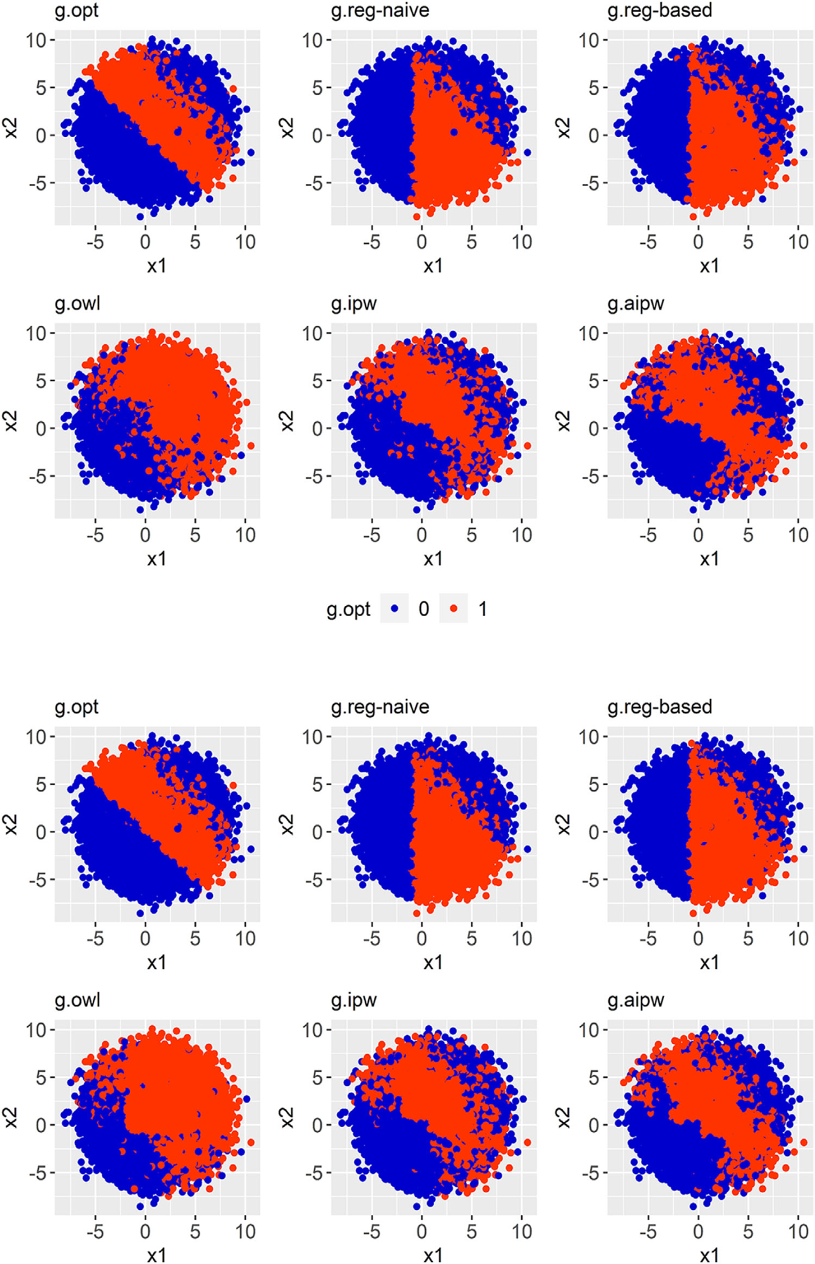
Note. Presence of effect modification on cost and only the outcome models are misspecified, WTP = $100K. The two panels are labeled as follows. Top: Medium HTE; Bottom: Large HTE. Each panel contains six figures: the very first figure shows the true decision boundary (gold standard), and the other five display the estimated decision boundaries that are given by five different methods.

FIGURE 2. Comparison of the decision boundaries of the estimated optimal ITRs.

Note. Absence of effect modification on cost and only the outcome models are misspecified, WTP = $100K. The two panels are labeled as follows. Top: Medium HTE; Bottom: Large HTE. Each panel contains six figures: the very first figure shows the true decision boundary (gold standard), and the other five display the estimated decision boundaries that are given by five different methods.

TABLE 2.

Comparison of the estimated mean outcomes (EMO) under different estimated optimal ITRs

EM	SM	HTE	$\mathbf{E}[{\mathit{Y}}^{{\mathit{g}}^{\text{opt}}}]$	$\mathbf{E}[{\mathbf{Y}}^{{\widehat{\mathbf{g}}}^{\text{Reg-naive}}}]$	$\mathbf{E}[{\mathit{Y}}^{{\widehat{\mathit{g}}}^{\text{Reg-based}}}]$	$\mathbf{E}[{\mathit{Y}}^{{\widehat{\mathit{g}}}^{\text{OWL}}}]$	$\mathbf{E}[{\mathit{Y}}^{{\widehat{\mathit{g}}}^{\text{IPW}}}]$	$\mathbf{E}[{\mathit{Y}}^{{\widehat{\mathit{g}}}^{\text{AIPW}}}]$
TM	1	M	15.672 (0.521)	15.265 (0.613)	14.991 (0.642)	13.401 (0.968)	14.393 (0.671)	14.822 (0.641)
		L	18.373 (0.531)	17.979 (0.614)	17.673 (0.649)	15.964 (0.985)	17.001 (0.728)	17.523 (0.635)
	2	M	15.672 (0.521)	13.757 (0.619)	13.675 (0.645)	13.401 (0.968)	14.393 (0.671)	14.791 (0.635)
		L	18.373 (0.531)	16.199 (0.646)	16.114 (0.674)	15.964 (0.985)	17.001 (0.728)	17.474 (0.641)
	3	M	15.672 (0.521)	15.265 (0.613)	14.991 (0.642)	12.950 (1.013)	14.163 (0.713)	14.763 (0.645)
		L	18.373 (0.531)	17.979 (0.614)	17.673 (0.649)	15.476 (1.089)	16.782 (0.747)	17.445 (0.645)
	4	M	15.672 (0.521)	13.757 (0.619)	13.675 (0.645)	12.950 (1.013)	14.163 (0.713)	14.702 (0.624)
		L	18.373 (0.531)	16.199 (0.646)	16.114 (0.674)	15.476 (1.089)	16.782 (0.747)	17.388 (0.642)
T	1	M	16.261 (0.521)	16.020 (0.558)	15.852 (0.568)	14.890 (0.694)	15.211 (0.616)	15.658 (0.581)
		L	18.991 (0.529)	18.756 (0.565)	18.564 (0.582)	17.516 (0.718)	17.864 (0.646)	18.374 (0.597)
	2	M	16.261 (0.521)	14.512 (0.565)	14.516 (0.573)	14.890 (0.694)	15.211 (0.616)	15.615 (0.586)
		L	18.991 (0.529)	16.984 (0.594)	16.985 (0.597)	17.516 (0.718)	17.864 (0.646)	18.328 (0.590)
	3	M	16.261 (0.521)	16.020 (0.558)	15.852 (0.568)	14.477 (0.766)	14.928 (0.657)	15.629 (0.584)
		L	18.991 (0.529)	18.756 (0.565)	18.564 (0.582)	17.047 (0.810)	17.533 (0.693)	18.342 (0.611)
	4	M	16.261 (0.521)	14.512 (0.565)	14.516 (0.573)	14.477 (0.766)	14.928 (0.657)	15.575 (0.581)
		L	18.991 (0.529)	16.984 (0.594)	16.985 (0.597)	17.047 (0.810)	17.533 (0.693)	18.273 (0.609)

Note. WTP = $100K. The indications of “EM,” “SM,” and “HTE” are the same as those in Table 1. The g^opt column represents the mean NMB under the true optimal regime (gold standard). ${\widehat{g}}^{\text{Reg}-\text{naive}}$, ${\widehat{g}}^{\text{Reg}-\text{based}}$, ${\widehat{g}}^{\text{OWL}}$, ${\widehat{g}}^{\text{IPW}}$, and ${\widehat{g}}^{\text{AIPW}}$ symbolize the estimated optimal ITR using naive regression method, regression-based method, OWL method, IPW method, and AIPW method, respectively. All the ITRs are based on a CE optimization strategy.

4 |. DATA ANALYSIS

Hypertension is the leading modifiable risk factor for CVD and death in the United States and worldwide. About 100 million U.S. adults have hypertension, which accounts for $80 billion in healthcare costs each year (Mozaffarian et al., 2014). Although the SPRINT evaluated the health benefits of an intensive SBP treatment (The SPRINT Research Group, 2015), decision making in healthcare policy weighs these benefits against the related medical expenditure. National population simulation models help quantify short- and long-term ramifications of healthcare decisions and inform clinical practice guidelines (Weinstein et al., 1987; Kahn et al., 2008; Abraham, 2013; Moran et al., 2015; Moise et al., 2016). With such a microsimulation model, Bress et al. (2017) projected long-term costs and health benefits of the SPRINT interventions and showed that the intensive SBP control is cost-effective across the full study population. However, it remains unclear if the treatment is cost-effective in individual patients. Following Bress et al. (2017), we applied our method to the microsimulation model that was populated with SPRINT participants to estimate the optimal individualized SBP control strategy. Specifically, a cohort of 10,000 patients was simulated by randomly sampling, with replacement, SPRINT participants. Clinical and economic outcomes were projected over 15 years, and the adherence and treatment effects were assumed to decrease over time after the first 5 years of follow-up. Approximately 60% of the subjects were censored at year 15. Our CE outcome, NMB, is a composite of restricted life-years and the total cost of hypertension treatment, CVD event hospitalizations, chronic CVD treatment, serious adverse events, and background healthcare costs. We used two WTP thresholds recommended by the American Heart Association, $50K and $100K per life-year (Anderson et al., 2014).

We estimated the classification weights using the top-performing AIPW approach suggested by our simulation study. To estimate the mean outcomes in the augmented terms of the AIPW estimator, we used the same two parametric models as those for restricted survival time and cost in the above simulation study. According to experts’ knowledge, 17 baseline covariates were preselected and employed to define both the main effect terms and covariate–treatment interaction terms. Then, we used these models to estimate the counterfactual NMBs under both the intensive and standard treatments. We conducted 10-fold cross-validation to prevent overfitting. In each iteration, we used 9/10 of the data as the training set to estimate the classification weights and build a tree model. Then, we predicted the optimal ITR on the rest 1/10 of the data (testing set). Moreover, we used the predicted potential outcomes on the testing set to calculate the NMB under the estimated optimal regime for each individual. We computed the bootstrapped 95% confidence interval with 1000 bootstrap resamples, in which the 2.5th and the 97.5th percentiles of the estimates were used as the lower and upper bounds, respectively.

Our conventional CE analysis indicates that the intensive SBP treatment is cost-effective on average and should be assigned to the full study population. However, our proposed method, the AIPW-based CE-ITR, considers the individual heterogeneity and suggests that the intensive control is cost-effective for 60% and 69% of the subjects when the WTP is $50K and $100K per life-year, respectively. To evaluate the gains on the mean NMB from considering individualized treatment rules, we compare the expected mean outcome under each regime. Table 3 shows that the mean NMBs under the personalized regimes are larger than those under the “one-size-fits-all” regimes across both WTP thresholds. The differences in mean NMBs when assigning all patients to the intensive versus control arm are consistent with our adherence assumption and prior findings (Bress et al., 2017). We present the most important variables for the optimal rule that ranked based on the average importance scores across 10 subsamples and 1000 bootstrap resamples. The importance score reflects the improvement that each variable makes in prediction. Given by the proposed method, Figure 3 displays that baseline SBP is the most predictive variable for the optimal CE-ITR across both WTP values, and this result is concordant with the existing findings that blood pressure is strongly associated with CVD risk reduction benefits from intensive treatment and added medical costs induced by intensive care (Basu et al., 2017; Bress et al., 2017).

TABLE 3.

The proportions of treated and estimated mean outcomes in a SPRINT-eligible cohort

	WTP	All patients assigned to intensive SBP control	All patients assigned to standard SBP control	AIPW-based CE-ITR (95% CI)
Proportion of treated	$50K	1	0	0.595 (0.368, 0.840)
	$100K	1	0	0.691 (0.423, 0.930)
Mean NMB outcome	$50K	435751	432320	437909 (434379, 441535)
	$100K	1056424	1042118	1058360 (1051240, 1066055)

Note. Our effectiveness measure is life-years and the follow-up length is 15 years. The rule of assigning all patients to intensive SBP control is the optimal rule from a conventional cost-effectiveness analysis based on the average treatment effect on NMB across the full study population. We conducted 10-fold cross-validation to avoid overfitting and computed the 95% CI using bootstrapping.

FIGURE 3. The importance of variables given by the AIPW-based CE ITR method.

Note. Abbreviations: Age: patient age; AntiHyperMed: number of antihypertensive medications; Aspirin: using aspirin at baseline; Black: black race; BMI: body mass index; CKD: chronic kidney disease; ClinicalCVD: clinical coronary vascular disease; DBP: diastolic blood pressure; Female: female gender; HDL: high-density lipoproteins; Hispanic: Hispanic race; SBP: systolic blood pressure; SmokerCurrent: current smoker; SmokerFormer: former smoker; Statin: using statins at baseline; TotCholesterol: total cholesterol; Triglycerides: baseline triglycerides level.

5 |. DISCUSSION

We have extended existing direct optimization methods to health economic evaluations so that flexible machine learning methods can be used to identify the most CE-ITR that is potentially complex and nonlinear. Consistent estimation of the optimal ITR using our method requires a consistent classifier and unbiased classification weights. Since Breiman et al. (1984) has shown the consistency of the classification tree method, our method provides consistent estimation as long as the NMB-based weights are unbiased. The Reg-based approach to estimating the classification weights relies on correct model specification for both restricted survival time and cumulative cost outcomes, which is often difficult to achieve. However, the proposed OWL, IPW, and AIPW methods depend less on modeling assumptions since they utilize weighting-based estimators. One downside of these inverse-weighting methods is that practical violation of the positivity assumption may produce extreme weights. Although the IPCW method is employed to account for right censoring, available partial information on CE contributed by censored subjects is essentially ignored. Such efficiency loss is a common concern of IPCW-based methods, and one possible improvement is to use a partitioned estimator for cost that utilizes partial information (e.g., cost history) of censored subjects (Bang and Tsiatis, 2000). In Section 2.4, even though the four classification weight estimators target different estimands, they are all potentially valid since their ultimate purpose is to capture the causal treatment effect on NMB at the individual level so that a classification tree is appropriately penalized. As there is little theoretical guidance on optimal weights (Zhou et al., 2015), we provided several alternatives and compared their performance numerically.

CE analyses are often used to identify an optimal risk threshold or subgroup for initiating treatment in populations with varying degrees of risk (Pandya et al., 2015; Kohli-Lynch et al., 2019). Our method improves current decision analyses by directly optimizing the ITR with regard to CE. Our method also provides a list of the most important variables in determining the optimal rule based on the variable importance produced by decision trees, which may help inform healthcare decision makers about allocating resources to ensure accurate collection of these variables. Direct application of the proposed methods to real data requires caution due to practical challenges in CE analyses. A frequent limitation is a short study time-horizon relative to the effects of the intervention. CE best practice guidelines recommend a lifetime horizon to capture relevant differences in both costs and health benefits, especially for chronic diseases. However, most clinical trials follow subjects for a limited number of years; so, the full survival curve is unknown and the difference in restricted mean survival times is often used to compare effectiveness (Lueza et al., 2016). On the cost side, limited follow-up time may induce biases when one treatment has a much higher initial cost but a lower subsequent cost than the other (Erickson and Winkelmayer, 2010). Another limitation that is specific to our SPRINT example is using uniform costs. We assigned every CVD event, medication, and serious adverse event a single dollar value, but these costs usually vary across different levels of health status, location, and time. Sensitivity analysis is a typical way to address such variation (Werner et al., 2012). Alternatively, one may adopt flexible cost generating models to capture the heterogeneity at a finer level (Franklin et al., 2019).

To the best of our knowledge, this is the first proposal on estimating the CE of ITR from a classification perspective. For simplicity, this paper is restricted to a one-time decision-making problem. However, one can extend our ideas to estimate the optimal dynamic treatment regime, which is a sequence of optimal personalized decision rules that when implemented over time will maximize the mean NMB at the end of the study (Murphy, 2003; Shen et al., 2017; Liu et al., 2018). Our proposal can also be extended to situations with multiple treatment arms as considered in single health outcome settings by Tao and Wang (2017). It can further be applied to other health economics evaluations such as cost–utility analysis (Leung et al., 2016) and cost–benefit analysis (Held et al., 2015), in which one replaces overall survival for other utility and benefit measures, respectively. We close by reiterating that when the goal is to inform healthcare priority setting and resource allocation, it is important that the estimation of optimal regimes incorporates cost, as we have shown in this study.

DATA AVAILABILITY STATEMENT

The data that support the findings in the Data Analysis Section are available to interested researchers upon reasonable request. Interested researchers can submit a one-to two-page research proposal and collaboration plan to Dr. Bellows (bkb2132@cumc.columbia.edu). The data are not publicly available due to privacy or ethical restrictions.

REFERENCES

- Abraham JM (2013) Using microsimulation models to inform U.S. health policy making. Health Services Research, 48, 686–695. [DOI] [PMC free article] [PubMed] [Google Scholar]
- Anderson JL, Heidenreich PA, Barnett PG, Creager MA, Fonarow GC, Gibbons RJ, et al. (2014) ACC/AHA statement on cost/value methodology in clinical practice guidelines and performance measures: a report of the American College of Cardiology/American Heart Association task force on performance measures and task force on practice guidelines. Journal of American College of Cardiology, 63, 2304–2322. [DOI] [PubMed] [Google Scholar]
- Breiman L, Friedman J, Stone CJ and Olshen RA (1984) Classification and Regression Trees. 1st edition. Boca Raton, FL: Chapman and Hall/CRC. [Google Scholar]
- Bang H and Tsiatis AA (2000) Estimating medical costs with censored data. Biometrika, 87, 329–343. [Google Scholar]
- Bress AP, Bellows BK, King JB, Hess R, Beddhu S, Zhang Z, et al. (2017) Cost-effectiveness of intensive versus standard blood-pressure control. New England Journal of Medicine, 377, 745–755. 10.1056/NEJMsa1616035. [DOI] [PMC free article] [PubMed] [Google Scholar]
- Basu S, Sussman JB, Rigdon J, Steimle L, Denton BT and Hayward RA (2017) Benefit and harm of intensive blood pressure treatment: derivation and validation of risk models using data from the SPRINT and ACCORD trials. PLOS Medicine, 14, e1002410. [DOI] [PMC free article] [PubMed] [Google Scholar]
- Cui Y, Zhu R and Kosorok M (2017) Tree based weighted learning for estimating individualized treatment rules with censored data. Electronic Journal of Statistics, 11, 107–117. [DOI] [PMC free article] [PubMed] [Google Scholar]
- Chen J, Fu H, He X, Kosorok MR and Liu Y (2018) Estimating individualized treatment rules for ordinal treatments. Biometrics, 74, 924–933. [DOI] [PMC free article] [PubMed] [Google Scholar]
- Cameron D, Ubels J and Norstrm F (2018) On what basis are medical cost-effectiveness thresholds set? Clashing opinions and an absence of data: a systematic review. Global Health Action, 11, 1447828. [DOI] [PMC free article] [PubMed] [Google Scholar]
- Erickson KF and Winkelmayer WC (2010) The challenges of cost-effectiveness analyses for the clinician. American Journal of Kidney Disease, 56, 1023–1025. [DOI] [PMC free article] [PubMed] [Google Scholar]
- Funk MJ, Westreich D, Wiesen C, Sturmer T, Brookhart MA and Davidian M (2011) Doubly robust estimation of causal effects. American Journal of Epidemiology, 173, 761–767. [DOI] [PMC free article] [PubMed] [Google Scholar]
- Franklin M, Lomas J, Walker S and Young T (2019) An educational review about using cost data for the purpose of cost-effectiveness analysis. Pharmacoeconomics, 37, 631–643. [DOI] [PubMed] [Google Scholar]
- Gillis JC and Goa KL (1996) Streptokinase. A pharmacoeconomic appraisal of its use in the management of acute myocardial infarction. Pharmacoeconomics, 10, 281–310. [DOI] [PubMed] [Google Scholar]
- Huang Y (2009) Cost analysis with censored data. Medical Care, 47, 115–119. [DOI] [PMC free article] [PubMed] [Google Scholar]
- Held PJ, McCormick F, Ojo A and Roberts JP (2015) A cost-benefit analysis of government compensation of kidney donors. American Journal of Transplantation, 16, 877–885. [DOI] [PMC free article] [PubMed] [Google Scholar]
- Kahn R, Robertson RM, Smith R and Eddy D (2008) The impact of prevention on reducing the burden of cardiovascular disease. Diabetes Care, 31, 1686–1696. [DOI] [PMC free article] [PubMed] [Google Scholar]
- Kent DM, Nelson J, Dahabreh IJ, Rothwell PM, Altman DG and Hayward RA (2016) Risk and treatment effect heterogeneity: re-analysis of individual participant data from 32 large clinical trials. International Journal of Epidemiology, 45, 2075–2088. [DOI] [PMC free article] [PubMed] [Google Scholar]
- Kohli-Lynch CN, Bellows BK, Thanassoulis G, Zhang Y, Pletcher MJ, Vittinghoff E, et al. (2019) Cost-effectiveness of low-density lipoprotein cholesterol level-guided STATIN treatment in patients with borderline cardiovascular risk. JAMA Cardiology, 4, 969–977. [DOI] [PMC free article] [PubMed] [Google Scholar]
- Lin DY, Feuer EJ, Etzioni R and Wax Y (1997) Estimating medical costs from incomplete follow-up data. Biometrics, 53, 419–434. [PubMed] [Google Scholar]
- Laber EB and Zhao YQ (2015) Tree-based methods for individualized treatment regimes. Biometrika, 102, 501–514. [DOI] [PMC free article] [PubMed] [Google Scholar]
- Lueza B, Rotolo F, Bonastre J, Pignon J and Michiels S (2016) Bias and precision of methods for estimating the difference in restricted mean survival time from an individual patient data meta-analysis. Medical Research Methodology, 16, 37. [DOI] [PMC free article] [PubMed] [Google Scholar]
- Leung W, Kvizhinadze G, Nair N and Blakely T (2016) Adjuvant trastuzumab in HER2-positive early breast cancer by SGE and hormone receptor status: a cost-utility analysis. PLOS Medicine, 13, e1002067. [DOI] [PMC free article] [PubMed] [Google Scholar]
- Li J, Vachani A, Epstein A and Mitra N (2018) A doubly robust approach for cost-effectiveness estimation from observational data. Statistical Methods in Medical Research, 27, 3126–3138. [DOI] [PubMed] [Google Scholar]
- Liu Y, Wang Y, Kosorok MR, Zhao Y and Zeng D, (2018) Augmented outcome-weighted learning for estimating optimal dynamic treatment regimens. Statistics in Medicine, 37, 3776–3788. [DOI] [PMC free article] [PubMed] [Google Scholar]
- Murphy SA (2003) Optimal dynamic treatment regimes. Journal of the Royal Statistical Society, 65, 331–366. [Google Scholar]
- Murphy SA (2005a) An experimental design for the development of adaptive treatment strategies. Statistics in Medicine, 24, 1455–1481. [DOI] [PubMed] [Google Scholar]
- Mozaffarian D, Benjamin EJ, Go AS, Arnett DK, Blaha MJ, Cushman M, et al. (2014) Heart disease and stroke statistics-2015 update: a report from the American Heart Association. Circulation, 131, e29–322. [DOI] [PubMed] [Google Scholar]
- Moran AE, Odden MC, Thanataveerat A, Tzong KY, Rasmussen PW, Guzman D, et al. (2015) Cost-effectiveness of hypertension therapy according to 2014 guidelines. New England Journal of Medicine, 372, 447–455. [DOI] [PMC free article] [PubMed] [Google Scholar]
- Moise N, Huang C, Rodgers A, Kohli-Lynch CN, Tzong KY, Coxson PG, et al. (2016) Comparative cost-effectiveness of conservative or intensive blood pressure treatment guidelines in adults aged 35–74 years: the cardiovascular disease policy model. Hypertension, 68, 88–96. [DOI] [PMC free article] [PubMed] [Google Scholar]
- Pandya A, Sy S, Cho S, Weinstein MC and Gaziano TA, (2015) Cost-effectiveness of 10-year risk thresholds for initiation of STATIN therapy for primary prevention of cardiovascular disease. JAMA, 314, 142–150. [DOI] [PMC free article] [PubMed] [Google Scholar]
- Qian M and Murphy SA (2011) Performance guarantees for individualized treatment rules. The Annals of Statistics, 39, 1180–1210. [DOI] [PMC free article] [PubMed] [Google Scholar]
- Robins JM and Greenland S (1992) Identifiability and exchangeability for direct and indirect effects. Epidemiology, 3, 143–155. [DOI] [PubMed] [Google Scholar]
- Schaubel DE and Wei G (2011) Double inverse-weighted estimation of cumulative treatment effects under nonproportional hazards and dependent censoring. Biometrics, 67, 29–38. [DOI] [PMC free article] [PubMed] [Google Scholar]
- Schulte PJ, Tsiatis AA, Laber EB and Davidian M (2014) Q- and A-learning methods for estimating optimal dynamic treatment regimes. Statistical Science, 29, 640–661. [DOI] [PMC free article] [PubMed] [Google Scholar]
- Shen J, Wang L and Taylor JM (2017) Estimation of the optimal regime in treatment of prostate cancer recurrence from observational data using flexible weighting models. Biometrics, 73, 635–645. [DOI] [PMC free article] [PubMed] [Google Scholar]
- Shen J, Wang L, Daignault S, Spratt DE, Morgan TM and Taylor JM (2018) Estimating the optimal personalized treatment strategy based on selected variables to prolong survival via random survival forest with weighted bootstrap. Journal of Biopharmaceutical Statistics, 28, 362–381. [DOI] [PMC free article] [PubMed] [Google Scholar]
- Thompson SG and Nixon RM (2005) How sensitive are cost-effectiveness analyses to choice of parametric distributions? Medical Decision Making, 25, 416–423. [DOI] [PubMed] [Google Scholar]
- Tian L, Alizadeh AA, Gentles AJ and Tibshirani R (2014) A simple method for estimating interactions between a treatment and a large number of covariates. Journal of the American Statistical Association, 109, 1517–1532. [DOI] [PMC free article] [PubMed] [Google Scholar]
- The SPRINT Research Group, (2015) A randomized trial of intensive versus standard blood-pressure control. New England Journal of Medicine, 373, 2103–2116. [DOI] [PMC free article] [PubMed] [Google Scholar]
- Tao Y and Wang L (2017) Adaptive contrast weighted learning for multi-stage multi-treatment decision-making. Biometrics, 73, 145–155. [DOI] [PubMed] [Google Scholar]
- Weinstein MC, Coxson PG, Williams LW, Pass TM, Stason WB and Goldman L (1987) Forecasting coronary heart disease incidence, mortality, and cost: the coronary heart disease policy model. American Journal of Public Health, 77, 1417–1426. [DOI] [PMC free article] [PubMed] [Google Scholar]
- Werner EF, Wheeler S and Burd I (2012) Creating decision trees to assess cost-effectiveness in clinical research. Journal of Biometrics and Biostatistics, S7, 1–3. [Google Scholar]
- Wang Y, Fu H and Zeng D (2017) Learning optimal personalized treatment rules in consideration of benefit and risk: with an application to treating type 2 diabetes patients with insulin therapies. Journal of the American Statistical Association, 113, 1–13. [DOI] [PMC free article] [PubMed] [Google Scholar]
- Zhao Y, Kosorok MR and Zeng D (2009) Reinforcement learning design for cancer clinical trials. Statistics in Medicine, 28, 3294–3315. [DOI] [PMC free article] [PubMed] [Google Scholar]
- Zhang B, Tsiatis AA, Davidian M, Zhang M and Laber E (2012a) Estimating optimal treatment regimes from a classification perspective. Stat, 1, 103–114. [DOI] [PMC free article] [PubMed] [Google Scholar]
- Zhang B, Tsiatis AA, Laber EB and Davidian M (2012b) A robust method for estimating optimal treatment regimes. Biometrics, 68, 1010–1018. [DOI] [PMC free article] [PubMed] [Google Scholar]
- Zhao Y, Zeng D, Rush AJ and Kosorok MR (2012) Estimating individualized treatment rules using outcome weighted learning. Journal of the American Statistical Association, 107, 1106–1118. [DOI] [PMC free article] [PubMed] [Google Scholar]
- Zhou X, Mayer HN, Khan U, and Kosorok MR (2015) Residual weighted learning for estimating individualized treatment rules. Journal of the American Statistical Association, 112, 169–187. [DOI] [PMC free article] [PubMed] [Google Scholar]
Associated Data
This section collects any data citations, data availability statements, or supplementary materials included in this article.
Supplementary Materials