

Abstract
The widespread development of new ultrasound image formation techniques has created a need for a standardized methodology for comparing the resulting images. Traditional methods of evaluation use quantitative metrics to assess the imaging performance in specific tasks such as point resolution or lesion detection. Quantitative evaluation is complicated by unconventional new methods and non-linear transformations of the dynamic range of data and images. Transformation-independent image metrics have been proposed for quantifying task performance. However, clinical ultrasound still relies heavily on visualization and qualitative assessment by expert observers. We propose the use of histogram matching to better assess differences across image formation methods. We briefly demonstrate the technique using a set of sample beamforming methods and discuss the implications of such image processing. We present variations of histogram matching and provide code to encourage application of this method within the imaging community.
I. Introduction
A conventional raw ultrasound image is formed by a delay-and-sum (DAS) beamforming of array channel data followed by envelope detection of the radio frequency or complex quadrature signals to visualize the amplitude modulated echo signal [1]. The resulting image values can span several orders of magnitude so the dynamic range is compressed using a function such as a logarithm or fractional exponentiation. Image post-processing is often applied to improve the image further, including smoothing background texture, sharpening edges, and enhancing contrast [2].
Historically, quantitative and visual evaluation of ultrasound images have been performed at different stages of this image formation process. Quantitative metrics are often computed on the raw images, allowing the beamformer to be analyzed in isolation from any image post-processing and providing certain statistical interpretations about imaging performance. Similarly, visual evaluation of images often benefits from dynamic range compression and image post-processing to remove artifacts of the image formation process. The vast majority of ultrasound procedures today are performed by human operators viewing compressed and processed images.
Modern ultrasound imaging research has produced a diverse set of imaging techniques that blur the line between the raw image and the displayed image. The widespread availability of open and programmable imaging systems [3] and improved computational capabilities have led to the proliferation of alternative image reconstruction algorithms. These algorithms range from using models to denoise and recover traditional delay-and-sum data [4]–[9], to weighting the DAS image with a correction factor [10]–[14], to replacing the coherent beamsum altogether with a non-linear image formation method [15]–[20]. The output images for different image formation methods do not necessarily have the same units as DAS; for instance, short-lag spatial coherence [17] produces images in units of correlation that are closer in appearance to the displayed (compressed) B-mode image. It is therefore important to standardize evaluation methods for new algorithm development.
Imaging algorithm development relies heavily on quantitative metrics because they allow different methods to be compared directly in specific imaging tasks. The superiority of a new method is often established by demonstrating improved performance across a panel of metrics in simulation, phantom, and in vivo studies. When the ground truth is known, metrics can measure the error directly (e.g., blood velocity, tissue stiffness, cardiac ejection fraction, the size of a structure). There are also numerous tasks in which the ground truth is unknown or does not exist, where the aim is instead simply to minimize or maximize the metric. Examples include the speckle signal-to-noise ratio, lesion conspicuity, and imaging resolution. However, these metrics are often heavily influenced by the types of transformations used to visualize ultrasound images, making it unclear whether the metrics convey a useful comparison between two imaging methods with different units [21]. A quantitative metric was recently proposed for comparing imaging methods with different units in the task of lesion detectability [22], representing an important step towards achieving fair comparisons of image quality. In the absence of additional transform-independent metrics for a wider range of tasks, a standardized methodology for visual evaluation takes on a greater importance.
Here, we describe a method for separating the evaluation of displayed dynamic range and information content in an image, enabling normalized comparisons between image formation methods. In Section II we review some common quantitative tools for image analysis and motivate the need for visual assessments. In Section III we present histogram matching as a tool for fair image comparison and describe several realizations useful for different tasks. In Section IV we demonstrate the application of this tool to compare several example imaging methods that could otherwise be subject to evaluation bias. In Section V we highlight potential pitfalls of this approach and discuss its impact on qualitative assessments.
II. Background
A. Common quantitative metrics
We begin with a survey of common quantitative metrics. Some metrics simply describe image features, while others have deeper statistical interpretations.
1). Texture Smoothness:
The characteristics of an image texture are assessed using the speckle signal-to-noise ratio (sSNR), defined as:
| (1) |
where μ and σ are the mean and standard deviation of brightness values within a region. When computed on uncompressed B-mode images from diffusely scattering targets (i.e. fully developed speckle), the image values are Rayleigh-distributed and sSNR ≈ 1.9 [23]. Higher values of sSNR indicate smoother speckle texture.
2). Lesion Contrast:
The contrast between two image regions is quantified using the contrast difference (CD) or contrast ratio (CR):
| (2) |
| (3) |
where μi is the mean value in region i. CD has units of the underlying image, whereas CR is dimensionless. CD is often used to compare log compressed images that are already in relative units (e.g. decibels), in which case it is identical to the CR of the uncompressed images expressed in the same units.
3). Lesion Detectability:
The contrast-to-noise ratio (CNR) [24] is measured as:
| (4) |
The CNR describes how visually distinguishable two regions are, combining both contrast and texture variance into one measure. Additionally, it has been found that target detectability is related to texture size (i.e. targets are more detectable within finer texture). When computed on raw B-mode images of diffusely scattering targets (i.e. fully developed speckle), the CNR including this resolution term represents the ideal observer in the task of lesion detection [25], [26].
The generalized contrast-to-noise ratio (gCNR) between two image regions is computed as the overlap between their histograms:
| (5) |
where f and g are the normalized histograms of two image regions. Unlike CNR, the gCNR provides a nonparametric measure of lesion detectability that is invariant to dynamic range transformations [22]. The gCNR is related to the minimum probability of error by the ideal classification algorithm; higher gCNR indicates a smaller probability of error.
4). Other Metrics:
Many quantitative metrics exist for other imaging tasks as well. For instance, in a linear imaging system the full-width at half-maximum (FWHM) of a point target describes the system resolution, whereas the side lobes of the point spread function describe the level and spatial extent of energy that is expected to produce off-axis scattering. Cystic resolution represents this spatial distribution of the point spread function by predicting target detectability as a function of lesion radius [27] and signal-to-noise ratio [28]. Contrast linearity [21], [29] has been proposed as a way to describe the accuracy of an imaging method in representing the native target contrast relative to the background irrespective of global transformations.
B. Impact of dynamic range transformations
Quantitative metrics are often computed on the uncompressed B-Mode images, while displayed images have typically undergone dynamic range compression, a type of monotonic transformation. However, most of the aforementioned metrics are not preserved under general monotonic transformations. Table I provides a list of several of these metrics and their theoretical properties under scaling, shifting, affine, and monotonic operations on an image with pixel values x. Among these, only the gCNR is preserved under all monotonic transformations.
TABLE I.
Image Metrics Preserved By Transformations
| Metric | Scale ax |
Shift x + b |
Affine ax + b |
Monotone h(x) |
|---|---|---|---|---|
| CD | X | ✓ | X | X |
| CR | ✓ | X | X | X |
| sSNR | ✓ | X | X | X |
| FWHM | ✓ | X | X | X |
| CNR | ✓ | ✓ | ✓ | X |
| gCNR | ✓ | ✓ | ✓ | ✓ |
Furthermore, the ranking of imaging methods from best to worst based on these metrics is generally not preserved under monotonic transformations. An imaging method that is quantitatively superior on raw images may be worse when the images have been compressed. Consequently, there may be a mismatch in quantitative metrics computed on raw images versus the actual displayed images. Fig. 1 gives a simple example of how the CD values and rankings are affected by a simple dynamic range transformation. Note that this effect is exacerbated when image formation or post-processing applies a different effective transformation to each image. For example, it is difficult to compare a log-compressed DAS image produced in a research lab to a commercial scanner image using an unknown compression and contrast-enhancing grayscale transformation.
Fig. 1.
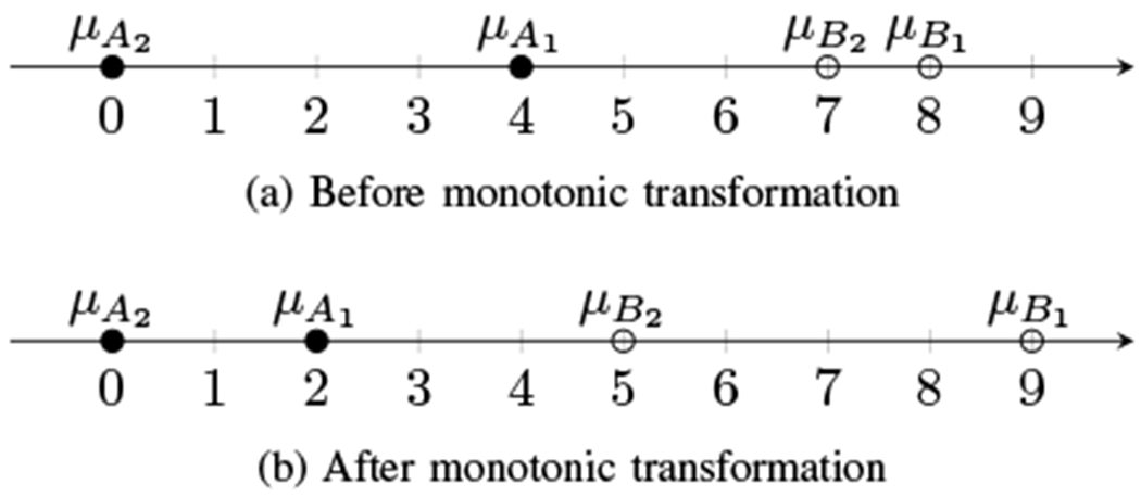
A simple example of how a monotonic transformation can affect contrast. Let μA1 and μA2 denote the mean values of image A in regions 1 and 2, shown plotted on a real number line. The contrast difference of method A is μA1 – μA2, i.e. the distance between the points. Before monotonic transformation, A has greater contrast than B. After monotonic transformation, B has greater contrast than A. Not only are the contrasts not preserved for A and B, the relative ranking of A and B contrast is not preserved.
C. Normalized image quality evaluation
These observations strongly motivate the need to evaluate images in the domains of their respective target applications. While quantitative metrics on raw images may be appropriate for applications such as computer-aided diagnosis or ideal observer analysis, imaging applications intended for human observers should also be evaluated using the displayed images. Clinical reader assessments are a common tool for evaluating the diagnostic value of new methods, often in the context of a particular clinical task. In cases when extensive reader studies are not feasible, simple quantitative metrics are needed to identify promising methods. However, dynamic range transformations can have a significant influence on quantitative metrics and may break the assumptions made by ideal observers [21], [22]. Whether visual assessment is performed by clinical readers or quantitative metrics, we require a robust and rigorous methodology for comparing new methods.
We propose the use of histogram matching to overcome the bias introduced by dynamic range transformations. Histogram matching is a family of techniques to ensure that two or more images are properly normalized for presentation [30]. This tool is often used in photography to compensate for the transfer function of an imaging sensor or varying lighting conditions. In the sections below, we describe the application of this tool to ultrasound images and its impact on common imaging tasks, including quantitative assessment.
III. Methods
In the subsections below, we present histogram matching for image normalization. In all cases, we consider an input image X and a reference image Y. The goal is to find a transformation of X that best matches Y. As we will show, the choice of transformation has a significant impact on the resulting perception and image quality metrics.
A. Partial histogram matching
The simplest transformations for histogram matching are the scaling and shifting operations:
| (6) |
| (7) |
These operations transform the histogram of X. Scaling affects the dynamic range of the image, whereas shifting the mean affects the overall brightness of the image. When combined, the resulting operation is referred to as an affine transformation, i.e., Xaffine = aX + b.
Histogram matching with affine transformations seeks the a and b that make the transformed image aX + b most similar to Y. In this work we choose a and b that match the mean μ and variance σ2 of X to that of Y :
| (8) |
| (9) |
This mean and variance matching method is easy to compute because it relies on simple descriptive statistics, and has the effect of maximizing the luminance and contrast terms of the structural similarity (SSIM) [31], a popular visual similarity metric for comparing images. For the same reason, it is somewhat robust to outliers in the distribution. Note that this method will only perfectly match two distributions that vary by at most these two moments, such as two images from Rayleigh distributions or Gaussian distributions or two images differing by a linear transformation. An alternative matching scheme is to minimize the L2 norm:
| (10) |
which as derived in Appendix A and produces weights:
| (11) |
| (12) |
where is the covariance of X and Y. It should be noted that other functions such as the L1 norm can also be used for optimization but may not have a closed-form solution for the affine coefficients.
Partial histogram matching fails to match the overall appearance of two images when their distributions significantly differ in shape (e.g. significant differences in higher-order moments such as skew and kurtosis). This also includes mixtures of distributions where the statistics of the overall data may be matched while the component distributions may not be.
B. Full histogram matching
For distributions not fully matched by the partial method, closer histogram matching can be achieved by considering a wider class of image transformations. Whereas partial histogram matching was restricted to the class of affine transformations, “full” histogram matching seeks any monotonic transformation that best matches the input probability density function (PDF) to the reference PDF. Unlike in the partial case, full histogram matching seeks to completely match the target distribution to the reference.
In practice, full histogram matching is accomplished by finding the mapping h from the input cumulative distribution function (CDF) FX to the reference CDF FY [32], [33]:
| (13) |
for discretely binned data. Interpolation is used between the bins to most closely match the overall distribution. The mapping function is then applied to the target distribution using interpolation to map individual pixel values:
| (14) |
The result should be that the target histogram matches closely with the reference histogram, depending on the resolution of binning.
C. Variations of histogram matching
There are important considerations for histogram matching:
1). Binning:
The limit of the binning process is to use individual pixels (1 pixel per bin). This “point” match can be simplified to rank-ordering the pixels of each image using a direct one-to-one mapping to replace the target pixel values. This process will exactly match the reference distribution but is particularly susceptible to outliers in the reference data since all values are replicated in the target.
2). Clipping:
Ultrasound data is commonly clipped for display by truncating the lower and/or upper range of the pixel values. For example, in a log-compressed B-mode image the lower end of the distribution extends as far as the noise floor of the system allows – well beyond useful information content. Clipping values lower than some threshold places the center of the distribution closer to the middle of the displayed dynamic range. In the above mean and variance matching, it is essential to operate on the whole image distribution (without clipping) so that the calculated statistics best represent the underlying data. This is not required for the full histogram matching approach, where the same percentage of the distribution will simply be mapped to the clipped value. For the case of matching a new image to a “black box” image, with access only to the display data with clipping applied, a full histogram matching approach may therefore be preferable.
3). ROI-based histogram matching:
If the reference image has extreme values (e.g. bright points or dark lesions), histogram matching would alter the entire target image to compensate. In these cases it may be useful to determine a transformation based on only a particular region of interest (ROI) and then to apply that transformation to the whole image. For example, a homogeneous speckle ROI within the image is expected to have a well-behaved distribution (Log-Rayleigh for a log compressed B-mode image). Histogram matching based on this ROI should produce a well-matched background “look and feel” to the images. Differences in other structures such as noise and acoustic clutter within hypoechoic lesions can then be assessed between the images. Alternatively, images could be matched to an analytical or reference distribution if a homogeneous ROI cannot be identified. When using an ROI, it may be possible that the full image contains pixel values outside the range of those in the ROI and therefore outside the mapping function. These values can be clipped to the mapping range, or we may employ linear extension of the mapping function to try to preserve the full dynamic range of the original target data. For example, a point target may have a brighter value than is present in the ROI speckle background and requires extrapolation to remain brighter in the matched image.
The above methods describe global dynamic range transformations and are the main focus of this work. Spatially adaptive matches are also possible by calculating the mapping function separately for multiple ROIs [34], but we will consider these to be more like image post-processing methods since they actually change the spatial information content of the image.
D. Test cases for evaluation
Sample data were acquired using the Verasonics Vantage 256 (Verasonics Inc., Kirkland, WA) using the P4-2v phased array transducer. Channel data were stored for individual element transmissions with center frequency 4.5 MHz for each element on the array. Synthetic aperture focusing was applied to coherently sum together the transmissions from all elements at each point in the image [35]. The ATS 549 general and small parts phantom (CIRS Inc., Norfolk, VA) was imaged to visualize speckle background, contrast lesion targets (−15 dB and −6 dB), and point targets.
To illustrate the impact of histogram matching across a wide spectrum of signal and image processing, we selected four representative imaging methods:
Conventional B-mode – Image formation by summation of the focused receive channel data, envelope detection (using the Hilbert transform), and log compression. This is the baseline case to compare against.
Square law detector – Same as conventional B-mode but envelope detection is performed by squaring the RF signal and low pass filtering, resulting in values approximately squared compared to the conventional B-mode (or doubled after log compression). This represents a case with little to no change in underlying information and only a simple (linear) dynamic range alteration.
Receive compounded – Incoherent spatial compounding, used to reduce speckle texture, by applying envelope detection to each receive channel individually before summation and log compression [36]. This represents a case of a true change in underlying information while retaining a similar but reduced dynamic range.
Short-lag spatial coherence (SLSC) – Image formation by averaging of complex cross-correlation of receive channel signals up to 10 elements apart after synthetic focusing [37], [38]. Unlike the above methods that are shown on a logarithmic scale, SLSC images are typically displayed on a linear scale between [0,1]. This represents a case of a true change in underlying information and image display units (i.e. based on correlation instead of signal amplitude).
Histogram matching was performed using 256 bins in all cases. The partial histogram matching method was implemented using the mean and variance matching of equations (8) and (9).
In order to make the histogram matching methods used in this work accessible to others in the imaging community, a MATLAB implementation and sample phantom data have been made available at https://github.com/nbottenus/histogram_matching (DOI: 10.5281/zenodo.4124190).
IV. Results
As a tool for fair qualitative image comparison, histogram matching is perhaps best evaluated by showing the images themselves for the various processed data sets. Fig. 2 shows the performance and characteristics of the partial and full histogram matching techniques both when applied based on the entire image and based only a speckle ROI in the middle of the image. All matched images are shown on the same dynamic range. For the cases that determined a histogram transfer function based on the ROI, any values outside the range of the transfer function were calculated using linear extrapolation.
Fig. 2.
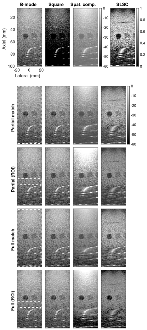
(top row) Original images for four image formation methods - Conventional B-mode, square law detector, receive spatial compounding, and short-lag spatial coherence (SLSC). SLSC is shown on a linear scale while the others are shown on a logarithmic scale (dB). (bottom four rows) Images after partial or full histogram matching, using either the full image or a speckle region of interest (indicated by dashed white box). All matched images are shown on the same logarithmic scale.
The original images show very different image characteristics. Compared to the conventional B-mode image, the square law image shows a darker background texture and finer point targets that stand out from the background. This appearance would fool both qualitative and quantitative assessments to say that resolution and contrast have improved. Spatial compounding shows the opposite effect, reducing texture especially within the darker lesion but with a haze over the image and reduced prominence of the point targets. SLSC, displayed on a linear scale rather than logarithmic, shows a bright background with high texture variance but extreme contrast of the lesions. SLSC also uniquely shows a small defect in the imaging phantom around 30 mm depth as a dark band, representing low spatial coherence.
The histograms for these images are shown in Fig. 3. The bottom plot shows the raw data as it was clipped and normalized for display, truncating the square law image's distribution and showing how the logarithmic images compare to the linear SLSC image. The clipping of the square law image produces the appearance of the point targets against a black background rather than showing any of the background texture. The spatially compounded image shows a compressed lower range, raising the image mean and creating the apparent haze. This compression potentially biases an observer to believe that lesion detectability has been reduced despite an accompanying smoothing of the background texture. The SLSC image shows the widest range including clipping on the low end, explaining the extreme appearance of the texture in the image and the dark lesion. This stretching of the dynamic range potentially biases visual comparisons against the B-mode image to conclude that the lesion detectability has improved despite an accompanying increase in the background texture variance.
Fig. 3.
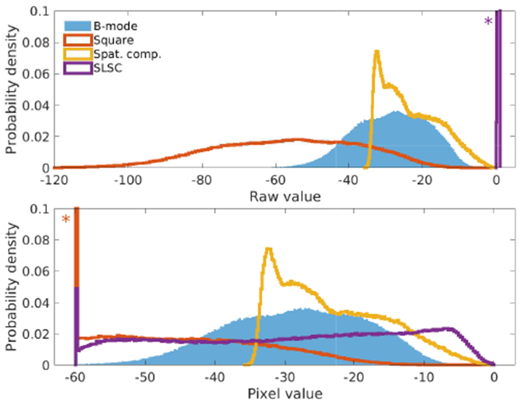
Histograms for the original images (top) using raw image data values (logarithmic except for the linearly-scaled SLSC image) and (bottom) after clipping of data to the displayed -60 dB dynamic range of the B-mode in Fig. 2. The SLSC image, normally displayed on a linear scale from 0 to 1, has been normalized to the displayed range for comparison. Asterisks indicate that the histogram extends past the displayed Y-axis.
Fig. 4 shows the image histograms after the proposed histogram matching strategies were applied. For each, histograms are shown for the entire image and for only the homogeneous speckle ROI identified in the images. In the original B-mode image, the background speckle region appears as a well-defined Log-Rayleigh distribution as expected. In all matching cases the square law data is almost exactly matched to the conventional B-mode. After partial matching, all four histograms have much more overlap. However, the differing shapes of the overall distributions for spatial compounding and SLSC result in differing means and variances for the speckle background. Conversely, partial matching of the distributions within the speckle ROI leaves large differences in the overall image. The square law data after logarithmic compression is approximately a linear transform of the B-mode data and is therefore matched by the partial (affine) technique for both the entire image and ROI. More complicated transforms, including nonlinear grayscale transforms such as sigmoidal compression for contrast enhancement [22], [39], require full matching. Full histogram matching, as expected, produces near-perfect overlap for the entire image and speckle background when referencing the entire image and ROI respectively. Matching the entire image leaves differences in the mean of the speckle background similar to the partial method, but the shapes of the distributions are more similar. Matching the speckle ROI leaves differences in the entire image, most notably in the low end of the SLSC image as it is stretched out to match the reference.
Fig. 4.
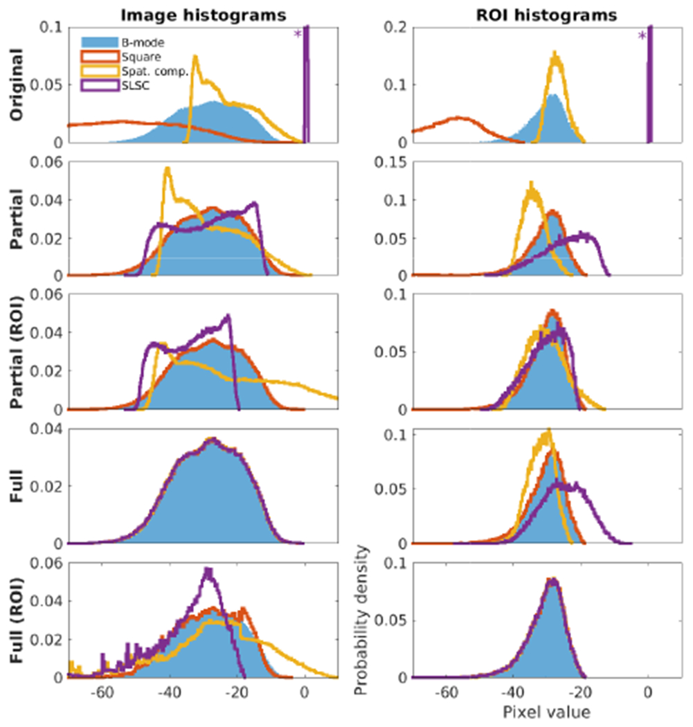
Results of the proposed histogram matching strategies corresponding to Fig. 2 evaluated for (left) the entire image and (right) the speckle ROI only. Asterisks indicate that the histogram extends past the displayed Y-axis. All histograms are shown with pixel value from [−70 10], although the histograms may extend further.
As discussed previously, imaging algorithms are often evaluated using point and lesion targets. These targets are shown in cross-section before and after image matching in Fig. 5. The measured FWHM (−6 dB for logarithmic images and 0.5 amplitude for linear images) for each case is given in Table II. Lesion targets were averaged over a 2 mm axial region to reduce noise. It is evident that without image matching the interpretation of these two targets is easily distorted by the original image display choices. For example, the square law detector shows both the best resolution and lesion contrast (at the expense of texture variance, only somewhat evident from these plots due to axial averaging). The reduced dynamic range of the spatial compounding method would make it seem the worst for both targets. However, after applying different matching schemes, the apparent performance of the image formation methods varies drastically. After partial matching based on the speckle ROI, spatial compounding appears to have the best resolution and lowest side lobes while performing comparably to the other methods in the lesion. It is evident that the center of the point target in SLSC becomes distorted under full histogram matching.
Fig. 5.
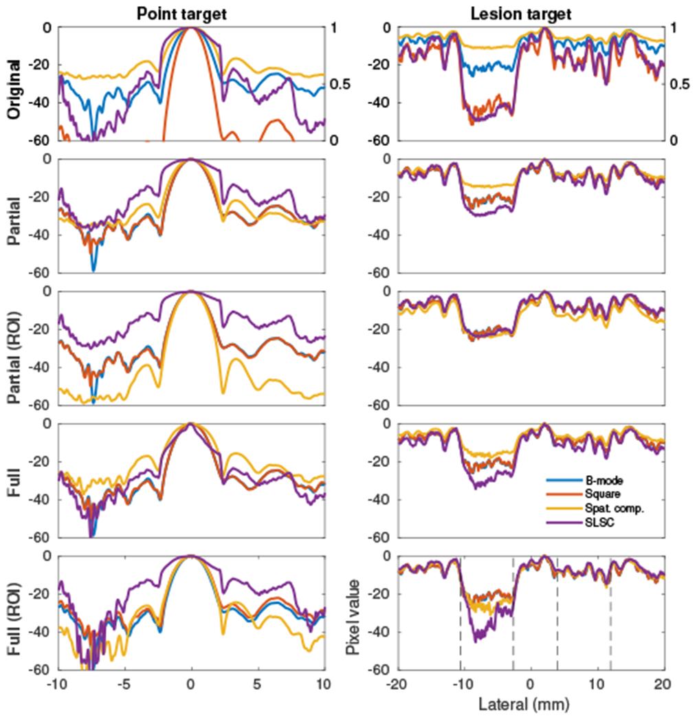
The four image formation methods compared in each plot for each matching method corresponding to Fig. 2. For the original images, SLSC is shown on a scale from 0 to 1. (left) Point target located at (−1, 84) mm, normalized to the maximum brightness. (right) Contrast lesion targets located at 50 mm depth, normalized to the maximum brightness. Lesion targets, nominally −15 and −6 dB, are approximately marked by black dashed lines in the bottom right plot.
TABLE II.
FWHM resolution (millimeters) for point targets in Fig. 5
| Matching | B-mode | Square | Spat. comp | SLSC |
|---|---|---|---|---|
| Original | 2.04 | 1.44 | 2.72 | 4.72 |
| Partial | 2.04 | 2.04 | 2.40 | 4.22 |
| Partial (ROI) | 2.04 | 2.02 | 1.88 | 4.36 |
| Full | 2.04 | 2.04 | 2.84 | 1.62 |
| Full (ROI) | 2.04 | 2.24 | 2.20 | 3.62 |
Four common image metrics used to evaluate imaging algorithms – sSNR, CR, CNR, and gCNR – are shown in Fig. 6 under the different matching strategies. Before matching, the speckle texture in the ROI (reflected by sSNR) is the smoothest in the spatially compounded image and most variable in the square law image. Note that partial matching by design matches the sSNR (μ/σ) of the chosen ROI exactly. After matching the whole image, compounding was observed to still produce the smoothest speckle texture while the other images were comparable. Lesion metrics were computed for the −15 dB lesion relative to the speckle ROI. The contrast in the original square law image was greatly exaggerated due to the stretched dynamic range. After matching, SLSC produced the greatest contrast (expressed as 1 – CR) while spatial compounding showed varying contrast depending on matching strategy. CNR was invariant to partial matching as described in Tbl. I with the exception of the square law image due to clipping. The difference in CNR between compounding and SLSC remained even after full matching but was slightly reduced. The gCNR was invariant to image matching as described in Tbl. I with the exception of the square law image due to clipping.
Fig. 6.
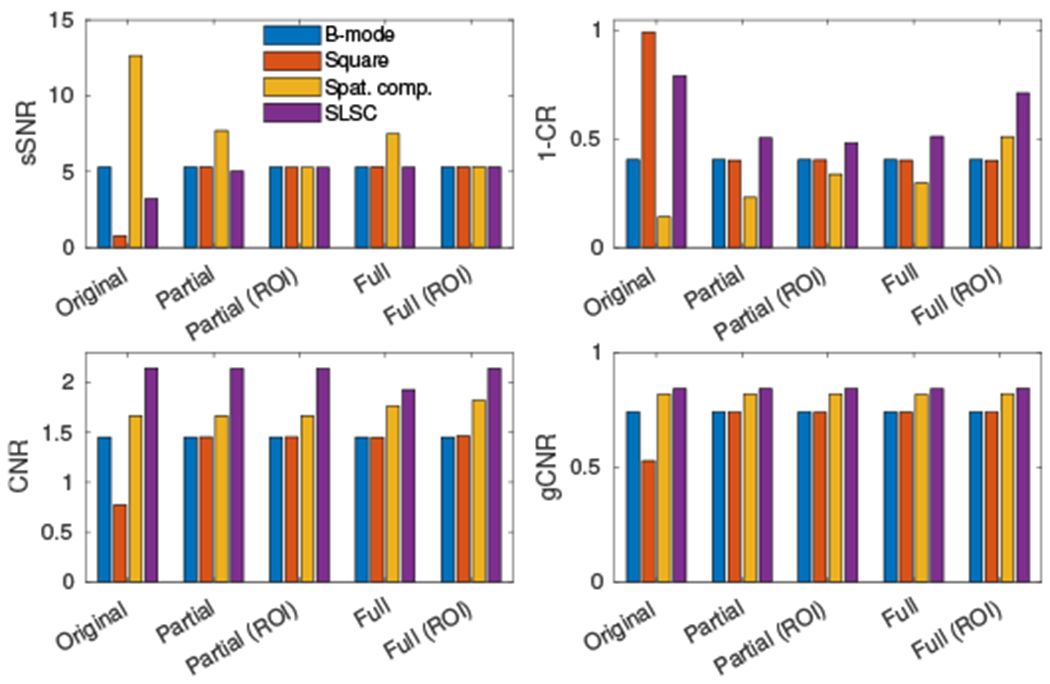
Image metrics calculated for the four image formation methods across matching methods for a −15 dB lesion and speckle background. Metrics are calculated using clipped and normalized image data as in the bottom of Fig. 3. Contrast is represented as 1 – CR such that a higher bar represents better contrast.
V. Discussion
Histogram matching provides a systematic approach for placing different imaging methods on a level playing field for visual evaluation. We have presented several variations, providing control over the matching transformation (partial versus full) and the matching region (local ROI versus whole image); one can further vary the matching objective function (mean and variance matching versus L2) and compensation for dynamic range clipping. As demonstrated in Fig. 2, histogram matching gives seemingly disparate imaging methods a similar appearance and reverses applied dynamic range transformations.
We expect that the most common use will be full histogram matching to a reference B-mode image using a homogeneous speckle ROI. B-mode speckle represents a known distribution that contains most of the echogenicity values expected in a typical clinical image and should enable a well-behaved transformation function between distributions of differing shapes. Image interpretation is then performed knowing that the speckle texture has been matched so that differences can be identified in target structures such as lesions. However, it should be recognized that point targets and anechoic structures may fall outside this distribution and are therefore limited by the chosen extrapolation of the histogram matching function. Partial matching may be more appropriate in circumstances where structure is included in the matching ROI or other situations where the overall shape of the histogram should be preserved. The method of matching should be clearly stated and justified to allow for appropriate interpretation of images. In some cases, it may be desirable to derive a different matching condition than presented here. For example, while the mean and variance affine match preserves sSNR, it is also possible to derive a transform that preserves lesion contrast that would highlight differences in the background texture.
There is not a universal “ideal” distribution for image matching. The structural content and therefore histograms of different clinical images vary widely between targets. For example, the liver appears as largely homogeneous speckle while the heart contains both brightly scattering tissue and low-scattering blood volume. Clinical imaging systems provide application-specific presets, which employ non-linear grayscale transfer curves that monotonically transform the displayed dynamic range to highlight structures of interest, maximize contrast between targets, and reject noise. These adjustments and therefore the ideal distribution for histogram matching vary widely based on imaging target and task.
The direction of image matching must also be selected with care. In Fig. 2, all images were matched to the compressed B-mode image. This is a natural choice for evaluating novel images in clinical settings where conventional B-mode is familiar. However, a goal of many novel imaging approaches is to detect features that are not visible in the B-mode image; features such as hypoechoic targets obscured by acoustic clutter may not be well-captured by the B-mode dynamic range and consequently may be lost during image matching. In these cases, it may be beneficial to perform matching in the other direction, i.e. the conventional B-mode to the novel image. This is especially important when images are clipped for display and novel information may be lost below a threshold that was selected to minimize noise in the original image. In the case of task-based metrics, improved performance across multiple metrics after matching in both directions could provide compelling evidence of superiority (note that for transform-invariant metrics such as the gCNR both directions are equivalent).
The histogram bins must be selected so as to allow proper observation of the dynamics of both histograms in order to enable an accurate mapping from one to the other. For instance, raw B-mode images will have a greater concentration of values near zero due to their high dynamic range, in which case the bins should be selected either on a logarithmic scale or after an appropriate dynamic range compression. It is also possible that quantization of the histogram bins may introduce some slight inconsistencies in the image. For the data in this study we found that 256 bins achieved consistent matching results, although fewer bins may be sufficient.
Evaluation, quantitative or qualitative, is best done on matched images at a stage that isolates the desired comparison. For example, comparison of beamformers as in this paper may best be performed on images formed before additional post-processing. Similarly, image post-processing should be assessed based on the same input data where possible. The interaction of each beamformer with a given post-processing method such as an adaptive speckle reduction or edge enhancement may vary, compounding the difficulty of interpretation if assessed together (although assessment with post-processing may ultimately be required for practical application [40]). Special attention should be paid to beamforming with neural networks [20] where a trained network may include some effective image post-processing not separable from the beamforming step. The histogram matching process is fundamentally the same in all cases, although the ROI to match may change based on the selected evaluation task.
Figs. 5 and 6 confirm the volatility of sSNR, lesion contrast, point target FWHM, and CNR under different dynamic range transformations. In particular, FWHM is easily confounded by image formation and processing. The rescaling of pixel values in the image can create an apparent change in resolution without reflecting the underlying information content of the data. Sparrow’s criterion [41], which measures the spacing at which two points form a flat plateau, is an alternative measure that unaffected by such dynamic range transformations. However, it still does not capture the full spatial distribution of energy in the tails of the point spread function and is more difficult to experimentally realize. These sensitivities underscore the critical need for a holistic view of image quality that combines task-based evaluation metrics with visual inspections and expert assessments. Histogram matching is a tool to minimize unintentional biases inherent to different imaging methods and represents one step towards achieving this goal.
VI. Conclusions
We have presented a methodology for the fair visual comparison of different ultrasound imaging techniques. Histogram matching provides a systematic approach for minimizing the visual differences between two images according to their histograms, and is meant to complement existing quantitative metrics. We have demonstrated partial (affine) and full (monotonic) histogram matching methods based on ROI and whole-image comparisons, and showed their effects on visualization as well as on traditional image metrics. Histogram matching is an integral tool to a comprehensive evaluation of imaging methods.
Acknowledgments
The authors would like to thank Gregg Trahey and Jeremy Dahl for their feedback in the preparation of this work.
This work is supported in part by grants R01-EB020040 and R01-EB013661 from the National Institute of Biomedical Imaging and Bioengineering.
Appendix
A. L2 affine matching
The L2 affine histogram match can be posed as minimizing the 2-norm of the difference between ax + b and y:
| (15) |
| (16) |
| (17) |
noting that 1T1 = N, xT 1 = Nμx, and yT 1 = Nμy. The partial derivative with respect to a is equal to zero when:
| (18) |
| (19) |
and the partial derivative with respect to b is equal to zero when:
| (20) |
| (21) |
| (22) |
| (23) |
| (24) |
where is the covariance of x and y and σ2x is the variance of x.
References
- [1].Cobbold RSC, Foundations of Biomedical Ultrasound, pp. 429–437, 492–504. Biomedical Engineering Series, Oxford University Press, 2007. [Google Scholar]
- [2].Ahman H, Thompson L, Swarbrick A, and Woodward J, “Understanding the advanced signal processing technique of real-time adaptive filters,” Journal of Diagnostic Medical Sonography, vol. 25, no. 3, pp. 145–160, 2009. [Google Scholar]
- [3].Boni E, Yu AC, Freear S, Jensen JA, and Tortoli P, “Ultrasound open platforms for next-generation imaging technique development,” IEEE Transactions on Ultrasonics, Ferroelectrics, and Frequency Control, vol. 65, no. 7, pp. 1078–1092, 2018. [DOI] [PMC free article] [PubMed] [Google Scholar]
- [4].Guenther DA and Walker WF, “Optimal Apodization Design for Medical Ultrasound Using Constrained Least Squares Part I : Theory,” IEEE Transactions on Ultrasonics, Ferroelectrics, and Frequency Control, vol. 54, pp. 332–342, Feb. 2007. [DOI] [PubMed] [Google Scholar]
- [5].Holfort IK, Gran F, and Jensen JA, “Broadband minimum variance beamforming for ultrasound imaging.,” IEEE Transactions on Ultrasonics, Ferroelectrics, and Frequency Control, vol. 56, pp. 314—25, February. 2009. [DOI] [PubMed] [Google Scholar]
- [6].Byram B, Dei K, Member S, Tierney J, and Dumont D, “A Model and Regularization Scheme for Ultrasonic Beamforming Clutter Reduction,” IEEE Transactions on Ultrasonics, Ferroelectrics and Frequency Control, vol. 62, no. 11, pp. 1–14, 2015. [DOI] [PMC free article] [PubMed] [Google Scholar]
- [7].Shin J and Huang L, “Spatial Prediction Filtering of Acoustic Clutter and Random Noise in Medical Ultrasound Imaging,” IEEE Transactions on Medical Imaging, vol. 36, no. 2, pp. 396–406, 2017. [DOI] [PubMed] [Google Scholar]
- [8].Luchies AC and Byram BC, “Deep Neural Networks for Ultrasound Beamforming,” IEEE Transactions on Medical Imaging, vol. 37, no. 9, pp. 2010–2021, 2018. [DOI] [PMC free article] [PubMed] [Google Scholar]
- [9].Brickson LL, Hyun D, and Dahl JJ, “Reverberation Noise Suppression in the Aperture Domain Using 3D Fully Convolutional Neural Networks,” in 2018 IEEE International Ultrasonics Symposium (IUS), (Kobe), pp. 1–4, IEEE, October. 2018. [Google Scholar]
- [10].Krishnan S, Rigby K, and O’Donnell M, “Efficient parallel adaptive aberration correction,” IEEE Transactions on Ultrasonics, Ferroelectrics and Frequency Control, vol. 45, no. 3, pp. 691–703, 1998. [DOI] [PubMed] [Google Scholar]
- [11].Hollman K, Rigby K, and O’Donnell M, “Coherence Factor of Speckle from a Multi-Row Probe,” IEEE Ultrasonics Symposium, 1999, pp. 1257–1260, 1999. [Google Scholar]
- [12].Li P-C and Li M-L, “Adaptive Imaging Using the Generalized Coherence Factor,” IEEE Transactions on Ultrasonics, Ferroelectrics and Frequency Control, vol. 50, no. 2, pp. 128–141, 2003. [DOI] [PubMed] [Google Scholar]
- [13].Camacho J, Parrilla M, and Fritsch C, “Phase coherence imaging,” IEEE Transactions on Ultrasonics, Ferroelectrics, and Frequency Control, vol. 56, pp. 958–974, May 2009. [DOI] [PubMed] [Google Scholar]
- [14].Long W, Bottenus N, and Trahey GE, “Incoherent Clutter Suppression using Lag-One Coherence,” IEEE Transactions on Ultrasonics, Ferroelectrics, and Frequency Control, pp. 1–1, 2020. [DOI] [PMC free article] [PubMed] [Google Scholar]
- [15].Shattuck D and von Ramm O, “Compound scanning with a phased array,” Ultrasonic Imaging, vol. 4, pp. 93–107, 1982. [DOI] [PubMed] [Google Scholar]
- [16].Seo CH and Yen JT, “Sidelobe suppression in ultrasound imaging using dual apodization with cross-correlation.,” IEEE Transactions on Ultrasonics, Ferroelectrics, and Frequency Control, vol. 55, pp. 2198210, October. 2008. [DOI] [PMC free article] [PubMed] [Google Scholar]
- [17].Lediju MA, Trahey GE, Byram BC, and Dahl JJ, “Short-lag spatial coherence of backscattered echoes: imaging characteristics.,” IEEE Transactions on Ultrasonics, Ferroelectrics and Frequency Control, vol. 58, pp. 1377–88, July 2011. [DOI] [PMC free article] [PubMed] [Google Scholar]
- [18].Matrone G, Savoia A, Caliano G, and Magenes G, “The Delay Multiply and Sum Beamforming Algorithm in Ultrasound B-Mode Medical Imaging,” IEEE Transactions on Medical Imaging, vol. 34, no. 4, pp. 940–949, 2014. [DOI] [PubMed] [Google Scholar]
- [19].Morgan MR, Trahey GE, and Walker WF, “Multi-covariate Imaging of Sub-resolution Targets,” IEEE Transactions on Medical Imaging, vol. 38, pp. 1690–1700, July 2019. [DOI] [PMC free article] [PubMed] [Google Scholar]
- [20].Hyun D, Brickson LL, Looby KT, and Dahl JJ, “Beamforming and speckle reduction using neural networks,” IEEE Transactions on Ultrasonics, Ferroelectrics, and Frequency Control, vol. 66, no. 5, pp. 898–910, 2019. Publisher: IEEE. [DOI] [PMC free article] [PubMed] [Google Scholar]
- [21].Rindal OMH, Austeng A, Fatemi A, and Rodriguez-Molares A, “The effect of dynamic range alterations in the estimation of contrast,” IEEE Transactions on Ultrasonics, Ferroelectrics, and Frequency Control, vol. PP, pp. 1–1, 2019. Publisher: IEEE. [DOI] [PubMed] [Google Scholar]
- [22].Rodriguez-Molares A, Marius O, Rindal H, and Jan D, “The Generalized Contrast-to-Noise ratio : a formal definition for lesion detectability,” IEEE Transactions on Ultrasonics, Ferroelectrics, and Frequency Control, pp. 1–12, 2019. [DOI] [PMC free article] [PubMed] [Google Scholar]
- [23].Wagner R, Smith S, Sandrik J, and Lopez H, “Statistics of Speckle in Ultrasound B-Scans,” IEEE Transactions on Sonics and Ultrasonics, vol. 30, pp. 156–163, May 1983. [Google Scholar]
- [24].Patterson M and Foster F, “The improvement and quantitative assessment of b-mode images produced by an annular array/cone hybrid,” Ultrasonic Imaging, vol. 5, no. 3, pp. 195–213, 1983. [DOI] [PubMed] [Google Scholar]
- [25].Smith SW, Wagner RF, Sandrik JFMF, and Lopez H, “Low contrast detectability and contrast/detail analysis in medical ultrasound,” IEEE Transactions on Sonics and Ultrasonics, vol. 3, no. 3, pp. 164—173, 1983. [Google Scholar]
- [26].Zemp RJ, Parry MD, Abbey CK, Insana MF, and Member S, “Detection performance theory for ultrasound imaging systems,” IEEE Transactions on Medical Imaging, vol. 24, no. 3, pp. 300–310, 2005. [DOI] [PMC free article] [PubMed] [Google Scholar]
- [27].Ranganathan K and Walker WF, “Cystic resolution: a performance metric for ultrasound imaging systems.,” IEEE Transactions on Ultrasonics, Ferroelectrics and Frequency Control, vol. 54, pp. 782–92, April. 2007. [DOI] [PubMed] [Google Scholar]
- [28].Guenther DA and Walker WF, “Generalized Cystic Resolution : A Metric for Assessing the Fundamental Limits on Beamformer Performance,” IEEE Transactions on Ultrasonics, Ferroelectrics and Frequency Control, vol. 56, pp. 77–90, January. 2009. [DOI] [PMC free article] [PubMed] [Google Scholar]
- [29].Dei K, Luchies A, and Byram B, “Contrast ratio dynamic range: A new beamformer performance metric,” IEEE International Ultrasonics Symposium, IUS, no. 1, pp. 0–3, 2017. [Google Scholar]
- [30].Gonzalez RC and Woods RE, Digital Image Processing. Upper Saddle River, N.J.: Prentice Hall, 2008. [Google Scholar]
- [31].Wang Z, Bovik AC, Sheikh HR, and Simoncelli EP, “Image Quality Assessment: From Error Measurement to Structural Similarity,” IEEE Transactions on Image Processing, vol. 13, no. 1, p. 14, 2004. [DOI] [PubMed] [Google Scholar]
- [32].Rolland JP, Vo V, Bloss B, and Abbey CK, “Fast algorithms for histogram matching: Application to texture synthesis,” Journal of Electronic Imaging, vol. 9, no. 1, p. 39, 2000. [Google Scholar]
- [33].Coltuc D, Bolon P, and Chassery J, “Exact histogram specification,” IEEE Transactions on Image Processing, vol. 15, no. 5, pp. 1143–1152, 2006. [DOI] [PubMed] [Google Scholar]
- [34].Pizer SM, Amburn EP, Austin JD, Cromartie R, Geselowitz A, Greer T, Romeny BTH, Zimmerman JB, and Zuiderveld K, “Adaptive Histogram Equalization and Its Variants,” Computer Vision, Graphics, and Image Processing, vol. 39, pp. 355–368, 1987. Publication Title: Computer Vision, Graphics, and Image Processing. [Google Scholar]
- [35].Karaman M and O’Donnell M, “Synthetic aperture imaging for small scale systems,” IEEE Transactions on Ultrasonics, Ferroelectrics and Frequency Control, vol. 42, no. 3, pp. 429–442, 1995. [DOI] [PubMed] [Google Scholar]
- [36].Trahey GE, Smith SW, and Von Ramm O, “Speckle pattern correlation with lateral aperture translation: Experimental results and implications for spatial compounding,” IEEE transactions on ultrasonics, ferroelectrics, and frequency control, vol. 33, no. 3, pp. 257–264, 1986. [DOI] [PubMed] [Google Scholar]
- [37].Dahl JJ, Hyun D, Lediju M, and Trahey GE, “Lesion Detectability in Diagnostic Ultrasound with Short-Lag Spatial Coherence Imaging,” Ultrasonic Imaging, vol. 133, pp. 119–133, 2011. [DOI] [PMC free article] [PubMed] [Google Scholar]
- [38].Bottenus N, Byram B, Dahl J, and Trahey G, “Synthetic aperture focusing for short-lag spatial coherence imaging,” IEEE Transactions on Ultrasonics, Ferroelectrics and Frequency Control, vol. 60, no. 9, pp. 1816–1826, 2013. [DOI] [PMC free article] [PubMed] [Google Scholar]
- [39].Thijssen J, Oosterveld B, and Wagner R, “Gray Level Transforms and Lesion Detectability in Echographic Images,” Ultrasonic Imaging, vol. 10, no. 3, pp. 171–195, 1988. Publisher: SAGE Publications. [DOI] [PubMed] [Google Scholar]
- [40].Huang O, Long W, Bottenus N, Lerendegui M, Trahey GE, Farsiu S, and Palmeri ML, “MimickNet, Mimicking Clinical Image Post-Processing Under Black-Box Constraints,” IEEE Transactions on Medical Imaging, vol. 39, no. 6, pp. 2277–2286, 2020. Publisher: Institute of Electrical and Electronics Engineers (IEEE). [DOI] [PMC free article] [PubMed] [Google Scholar]
- [41].Sparrow C, “On spectroscopic resolving power,” Astrophysical Journal, vol. 44, pp. 76–86, 1916. [Google Scholar]