Topoly: Python package to analyze topology of polymers

Abstract

The increasing role of topology in (bio)physical properties of matter creates a need for an efficient method of detecting the topology of a (bio)polymer. However, the existing tools allow one to classify only the simplest knots and cannot be used in automated sample analysis. To answer this need, we created the Topoly Python package. This package enables the distinguishing of knots, slipknots, links and spatial graphs through the calculation of different topological polynomial invariants. It also enables one to create the minimal spanning surface on a given loop, e.g. to detect a lasso motif or to generate random closed polymers. It is capable of reading various file formats, including PDB. The extensive documentation along with test cases and the simplicity of the Python programming language make it a very simple to use yet powerful tool, suitable even for inexperienced users. Topoly can be obtained from https://topoly.cent.uw.edu.pl.

Introduction

The history of science provides dozens of cases when the properties of matter were dictated not by its composition, but rather by its spatial arrangements. In the 20th century, great attention was paid to monitor the chirality of the compounds. Recently, researchers moved one step further and focused on the analysis of the influence of the topology on the properties of polymers. In particular, the effect of knots, slipknots and links in linear polymers was studied in designed compounds [3, 5, 6, 55, 62, 66], DNA [4, 57, 59] and proteins [10, 13, 19, 37, 63, 67]. The inclusion of branching points showed the existence of the -curve topology, lasso motif or cystine knots [14, 18, 21, 49], where the depth of the piercing affects the properties of the polymer [3, 51].

However, for complex structures, the identification of the topologically nontrivial motif becomes a time-consuming and hard task even for specialists. Therefore, a tool automatically identifying the nontrivial topology is required. For some topologies (usually knots or links), one may use some dedicated web servers [16–18, 32, 39, 41, 42, 64], plugins [25, 26, 43] or stand-alone packages [23, 31, 33]. However, such an approach is not sufficient when one needs to perform a meticulous analysis of the whole library of polymer structures, use non-standard methods or analyze new topologies (such as branched polymers). To address this need, we have developed a flexible and powerful tool—the Topoly package (https://topoly.cent.uw.edu.pl).

Topoly is a Python3 package, allowing one to identify and analyze any polymers’ topology studied so far. Apart from standard knot-determining techniques (Alexander, Conway, Jones and HOMFLY-PT polynomials [2, 34]) it includes less-known methods (Kauffman and APS Brackets, Kauffman and BLM/Ho polynomials [11, 20, 30, 35, 36]), a polynomial for the analysis of spatial graphs (Yamada polynomial [65]), minimal surface analysis to identify the lasso topology [49] or the Gauss linking number (GLN) [46, 47, 56]. Exemplary structures, which can be analyzed with Topoly, are presented in Figure 1. To study statistics, or simply to test the behavior of the functions provided, the user may also generate random loops and lassos (tadpoles), -curves, two-component links and handcuff graphs (dumbbells).

Figure 1.

The exemplary structures, which can be identified using the Topoly package, and the methods suitable for their detection (below the schemes). The schemes present (from left to right) knot, Hopf link, slipknot, lasso, -curve, handcuff graph and a random polymer with 20 steps.

Apart from self-generated structures, Topoly as a versatile tool accepts structures provided as a set of coordinates in various formats (XYZ, PDB, mmCIF, Mathematica and other) or as an abstract code (Planar Diagram or Ewing–Millett [24] code). For open structures (such as protein chains), the package provides the option of chain closure with various methods [48, 53]. As usual in case of a Python package, Topoly’s results can be easily captured and parsed further according to the needs of the user. Topoly comes with a thorough manual (including the description of all functions) and a tutorial project (https://github.com/ilbsm/topoly_tutorial) that includes real-life examples of its usage.

Getting started

Topoly is available for Python3 running on 64-bit Linux or Mac OS X. It is distributed using the standard Python package manager—PyPI—and can be easily installed by invoking pip install topoly, provided a recent version of the pip installer is used.

The easiest way to get started with Topoly is to download or clone the tutorial project that we provide at https://github.com/ilbsm/topoly_tutorial and follow the three-step instructions in the README.

Topoly features

Input files and format translation

The main function of Topoly is to analyze the topology of the structure given either as 3D coordinates (PDB, mmCIF, XYZ, Mathematica formats) or as an abstract code (Planar Diagram or Ewing–Millett [24] code). In case the structure is given as PDB or mmCIF file (e.g. directly from the RCSB database), the coordinates of atoms are extracted. The user may also supply the spatial graphs (with branching points) with each arc separated by a line without coordinates.

The coordinates and the codes for the structures are stored in the memory and can be written out in the desired format. In particular, this option can be used to translate between the formats, e.g. PDB Mathematica, or to obtain the abstract representation, e.g. Mathematica PD code. Currently, the recreation of the coordinates (PD Mathematica) is not possible, if the coordinates were not given.

Knot and link analysis

The knots and links are in general well defined for closed components. For such structures, the user may use the Alexander, Conway, Jones, HOMFLY-PT polynomial, and Kauffman Bracket but also less-known Yamada, Kauffman and BLM/Ho polynomials, and APS Bracket, which, to our best knowledge, are not implemented anywhere else (Table 1). In Figure 2 is our proposition when to use each invariant. By default, the result of each function is the knot type (e.g. ) corresponding to the structure analyzed. The knot type is obtained by comparing the polynomial value with the local polynomial library, containing all knots and links (prime and composite) with up to eight crossings. The user may also request the chirality of the knot and link using the keyword argument chiral=True. In such case, the structure type is returned with a sign (e.g. ) if possible, where the Doll–Hoste [22] convention is used for links.

Table 1.

Table of available invariants and their capabilities of distinguishing different chiralities, links, and spatial graphs. They are sorted by relative speed when running with deterministic closure and no subchain analysis. Note that Conway and Jones polynomials are relatively faster, when using probabilistic closure or during extensive subchain analysis

Invariant	Speed rank	Chirality	Links	Spatial graphs
Alexander polynomial	1st	no	no	no
HOMFLY polynomial	2st	yes	yes	no
Conway polynomial	3rd	no	no	no
Jones polynomial	3rd	yes	yes	no
Yamada polynomial	4th	yes	yes	yes
BLMHo polynomial	4th	no	yes	no
Kauffman polynomial	4th	yes	yes	no
Kauffman bracket	5th	yes	yes	no
APS bracket	5th	yes	yes	yes

Figure 2.

Decision tree with our proposition of choosing optimal invariant for topology check. We recommend usage of other invariants only for more specific goals, e.g. identification of topologies with more than eight crossings and theoretical research of topological invariants.

Instead of the link type, the user may request the original, untranslated polynomial value (e.g. ) with the keyword argument translate=False. This option may be used, e.g. to calculate the polynomial for more complicated structures (e.g. with nine crossings). Such a result can be then stored in a user-created (external) dictionary of polynomials and included in further calculations.

In the case of open-chain structures (such as proteins), the chain usually needs to be closed first in order to analyze its topology. The Topoly package provides several closure methods, including stochastic closure, in which the topology is calculated for many random closures (more examples are discussed below). In such cases, the result of the calculation is a dictionary with the obtained types of topologies and their probabilities (e.g. {’’: 0.6, ’’: 0.3, ’’: 0.1}).

Spatial graphs

One of the key features of the Topoly package is the possibility to analyze the topology of spatial graphs, i.e. polymers with branching points. Such structures appear naturally in biology (e.g. glycogen, cystine knots and cyclotides, lasso proteins and peptides [29, 44, 49] or replicating cyclic DNA [1, 52]). The analysis of such structures may be performed using, e.g. the Yamada polynomial or APS bracket, to the best of our knowledge implemented solely in the Topoly package. In particular, one can analyze the topology of -curves or handcuff graphs (Figure 1). The Topoly package contains a local library of Yamada polynomials for all prime and composite -curves as well as handcuff graphs with up to seven crossings.

Spanning minimal surface and detection of surface piercings

Another feature of the Topoly package is the ability to construct a triangulated minimal surface spanning a closed loop. The coordinates of the surface-forming triangles may be exported or used to analyze piercings through the loop (minimal surface method). This technique was used to analyze polymer rings in melt [58] and to analyze the organization of chromatin domains [45] or to identify complex lasso proteins [49], where the tail pierces the loop closed by a disulfide bridge (Figure 1). To perform such analysis, the user has to specify the indices of the loop closing bridge. In the case of PDB or mmCIF files, the bridges are recognized automatically. By default, only the disulfide bridges are taken into account but the user may also include other covalent bridges (e.g. amide) or the bridges mediated by ions.

Alternatively, the piercings through the loop may be analyzed using the GLN. Originally, the linking number counts how many times one loop pierces the other. It was initially defined only for a closed loop; however, its integral definition may be also extended to open structures [9]. In such a case, fractional values are obtained and the significantly nonzero value of the GLN should indicate a piercing [50]. The user may analyze either two parts of the same chain (specified by the indices) or two separate chains. The GLN was already used to study the conformation and entanglement of proteins [7, 8, 13, 27, 46, 47] and chromosomes [60].

Analysis of subchains

Apart from the analysis of the whole structure, in case of the knotted chain and GLN approach, one can also analyze the entanglement of each subchain. As the subchain is specified by two indices—begin and end—the information about the topology of each subchain can be encoded in a two-dimensional matrix, indexed by the beginning and the end of the subchain. Such an approach in the case of knots is called the knot fingerprint matrix (Figure 3) [37, 61]. The representation of proteins’ chains in the form of a matrix leads to the discovery of slipknots (the overall unknotted structures which have a nontrivial subchain) and a strict conservation of complex knotting patterns (compositions of slipknots) within and between several protein families, despite their large sequence divergence [61]. The GLN matrix was used, e.g. to spot high winding of the chain around closed loops [50].

Figure 3.

The exemplary matrices obtained with Alexander polynomial (left and middle) and GLN from Topoly package. Structures analyzed from left to right: slipknot, composite knot formed by artificial structures and lasso formed by hyperthermophilic archaeal RNase HI (PDB code 2ehg). The visualization of the analyzed structures was placed in the top-right corners of the matrices. In case of the 2egh structure (right panel) the loop (in blue) is closed by a cysteine bridge (orange) between Cys58-Cys145 and pierced by the N-terminal tail (red).

For the GLN and each knot polynomial function, the matrix analysis may be invoked by using the keyword matrix=True. By default, the matrix is presented as a dictionary indexed by each subchain. The user may, however, plot the matrix and save in a desired format (PNG, SVG, PDF).

Structure importing, generating and finding

Apart from the library of polynomial values, the Topoly package includes also a library of planar diagram codes for knots/links with up to eight crossings and -curves and handcuff graphs for up to seven crossings. Therefore, the user has a vast library for his/her own analysis.

Alternatively, Topoly allows sampling of random structures. This option may be useful to study the statistics of random chains. Topoly includes the possibility to sample random walks, loops, lassos, -curves, two-component links and handcuff graphs (Figure 1), generated using Cantarella et al.’s [12] algorithm. The structures may be presented as a Python list or the coordinates may be saved to separate files.

On the other hand, the user may analyze complex, multi-branched polymers (like proteins with disulfide bridges), extracting loops, -curves, links and handcuff graphs using the appropriate find_ function (Figure 4). Such an approach was already used to find -curves in proteins [14].

Figure 4.

The exemplary results of finding functions implemented in Topoly. For the exemplary structure (top-left) with three disulfide bonds (marked as orange stripes) exemplary results of find_loops, find_thetas and find_handcuffs are presented. In total, four loops, one -curve and eight handcuffs were found in this case.

Finally, for a given matrix fingerprint, the user may also identify the representative subchains, which may differ in topology. Such analysis is currently used in the KnotProt database to prescribe the knot fingerprint, as a concatenation of topological types of each representative subchain (e.g. in the case of an -haloacid dehalogenase protein). In Topoly, the representative subchains with their topologies are obtained using the find_spots function.

Programmed speedup

Due to the run-time complexity of some algorithms (e.g. calculating the topology of every possible subchain), the Topoly calculation is accelerated on various levels of the implementation. On the algorithmic level, the sampling of subchains is optimized. The knot fingerprint matrix calculation is divided into two parts. In the first one, only a subset of points is calculated. The size of the subset is controlled by the density parameter (the higher the value, the less points are calculated in the first step). The surroundings of these points are calculated in the second step only if a nontrivial topology was identified in the first step. Moreover, the planar diagram codes of the structures are compared with the local library; therefore, only the yet unknown structures are calculated. Furthermore, the calculation of the matrix is done in parallel (governed by the keyword run_parallel) using all the computational power available (unless the user limits the number of cores by setting the value of parallel_workers). Finally, for the Alexander polynomial (dedicated to matrix calculation) the analysis may be also done using the GPU units that support the CUDA technology.

Other options

Apart from the topological analysis, the Topoly package provides some auxiliary functions helpful in the analysis. In particular, for an open structure, the user may close it (with close_curve function) using several methods, including closure on a big sphere surrounding the structure, extending rays in one direction or extending the termini from the center of the mass (Figure 5). The closed structure may be then reduced (reduce_structure function) with the implementation of the Koniaris–Muthukumar–Taylor algorithm [40, 63] or by a chain of Reidemeister moves. To visualize the effect of chain closure or reduction, one may use the function plot_graph which opens the Matplotlib window in which the structure is shown (Figure 5).

Figure 5.

The exemplary closure methods. From left to right—two-point closure on the sphere (two points are randomly chosen on a large sphere and connected with an arc visible in the front), extending rays in one direction, extending the termini from the center of the mass, and connected with an arc visible in the front. In all three panels, the same structure (with PDB code 1j85) was closed. The structures were drawn with the Topoly implemented function plot_graph.

For a structure in a given format (e.g. Mathematica-generated file), Topoly allows one to translate it into different supported formats (e.g. PDB file) using the translate_code function. In particular, this way one can obtain, e.g. the planar diagram code of a 3D structure.

By default, the obatined matrix fingerprint is presented as a Python dictionary. As the user may want to plot the result on their own, it may be translated to a string (KnotProt format) or a list applicable to Matplotlib or Gnuplot using the translate_matrix function.

Finally, the user may also use Topoly to find a match for a given polynomial in the local library using the find_matching function. This may be used to find the link chirality if the appropriate polynomial was calculated with some external software.

Exemplary cases

We will present four exemplary cases.

• (i) Calculation of knot topology for UCH protein (PDB code 2len, chain A, model 2) with the Conway polynomial.

  >>>from topoly import conway, Closure

  >>># statistics of knots for different closures

  >>> print(conway(’2len.pdb’, pdb_chain=’A’,pdb_model=2))

  {’5_2’: 0.61, ’0_1’: 0.22, ’3_1’: 0.035, ’4_1’: 0.035, ’Unknown’: 0.030, ’5_1’: 0.025, ’7_6’: 0.015, ’6_1’: 0.01, ’7_3’: 0.01, ’7_4’: 0.005, ’8_4’: 0.005}

  >>> # the explicit Conway polynomial for closed structure

  >>> print(conway(’2len.pdb’, translate=False, poly_reduce=False, closure=Closure.MASS_CENTER))

  1 + 2z^2

  z We assume the file ’2len.pdb’ is stored locally during the analysis after having been downloaded from the RCSB server. We explicitly write the parameters. First, the statistics of knots are obtained. In particular, the knot is obtained with a probability of 0.61 (in 61% of closures, Figure 6A). In the last step, we calculate the polynomial value () for the structure closed with arms extended from the center of mass. We do not translate the polynomial value to a matching knot type (). This analysis shows the diversity of the detected topology which is a consequence of using a statistical approach to close the chain as well as of the internal complexity of the protein backbone.

• (ii) Plotting and analyzing the knot fingerprint matrix for UCH37 (PDB code 4i6n).

  >>> from topoly import alexander, homfly, find_spots

  >>> # calculating and plotting the matrix

  matrix_result = alexander(’4i6n.pdb’, matrix_map=True, map_arrows=False)

  # finding the spot centers

  spots = find_spots(matrix_result, map_cutoff=0.36)

  >>> print(spots)

  ’5_2’: [(2, 228)], ’3_1’: [(5, 173), (6, 211)]

  >>> # establishing chirality

  >>> for knot in spots.keys():

  ... for spot in spots.get(knot):

  ... print(homfly(’4i6n.pdb’, chain_boundary=[spot], chiral=True, closure=Closure.MASS_CENTER))

  (2, 228) -5_2

  (5, 173) -3_1

  (6, 211) -3_1

  We assume the file ’4i6n.pdb’ is stored locally during analysis and the indices are renumbered to start from 1. The matrix is calculated with the Alexander polynomial (the fastest, devoted to matrix calculations). Next, the spots (representative subchains) are identified (with indices 2–228 for knot, 6–211 for slipknot and 5–173 for the most deeply embeded slipkot; Figure 6B). In the last step, we analyze the chirality of each subchain found in find_spots step. It turns out that the representative subchain with the topology has the same chirality. As a consequence, the composition of these commands allows one to determine the fundamental topological properties of proteins, such as depth of knots and slipknots, their locations, as well as to compare the entanglement between different proteins. Similar properties in the case of lassos can be determined based on the GLN matrix.

• (iii) Calculating the lasso type for all the loops in cerato-platanin (PDB code 3sum).

  >>> from topoly import lasso_type

  >>># gathering information about lassos

  >>> lassos = lasso_type(’3sum.pdb’, more_info=True)

  >>> for lasso in lassos.keys():

  ... loop = lasso

  ... motif = lassos[lasso][’class’]

  ... piercing_N = lassos[lasso][’crossingsN’]

  ... piercing_C = lassos[lasso][’crossingsC’]

  ... print(loop, motif, piercing_N + piercing_C)

  (43, 80) L+1C [’+97’]

  (83, 145) L+1N [’+72’]

  (144, 153) L0 []

  We assume the file ’3sum.pdb’ is stored locally during the analysis. We calculate the lasso types and in the last step, we print the result, loop by loop, including the loop-delimiting indices, the topology of the lasso and the indices of piercing residues. The Mathematica visualization of surface files obtained for nontrivial lassos are shown in Figure 6C. The composition of such commands allows for a comprehensive analysis of the lasso type topology—location of the loop and piercings and depth of piercings. Both parameters are important to study kinetics pathways [28, 54], stability [38] and statistical and biological properties [15].

• (iv) Generation of loops for statistics.

  >>> from topoly import generate_loop, jones

  >>> # for statistic analysis

  >>> from collections import Counter

  >>> # generating loops

  >>> loops = generate_loop(100, 1000, output=’list’)

  >>> # establishing the topology of the loops

  >>> result = [jones(loop, closure=Closure.CLOSED) for loop in loops]

  >>> # printing the statistics

  >>> print(Counter(result)) Counter({’0_1’: 700, ’3_1’: 170, ’4_1’: 27, ’3_1#3_1’: 23,...

  We generate 1000 loops with 100 nodes each and calculate the corresponding knot statistics. For a better visualization, the results summarized using extarnal tool—Counter. The results are presented in Figure 6D. Such analysis can be useful in the comparison of statistical properties between, e.g. proteins and random polymers.

Figure 6.

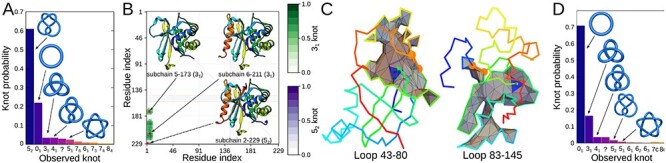
The graphical result of the exemplary cases. (A) The histogram of knots obtained for different closures of the UCH protein (PDB code 2len, test case 1). (B) The knot fingerprint matrix obtained for UCH37 protein (PDB code 4i6n, test case 2). (C) The surfaces spanned on the main chain of cerato-platanin (PDB code 3sum) closed by bridges 43–80 (left panel) and 83–145 (right panel) with the piercings indicated by the blue triangle (test case 3). The third bridge results in a trivial lasso. The surfaces are visualized with Mathematica. (D) The histogram of different knot types obtained for 1000 random loops with the length 100 (test case 4).

Test project and package manual

The further growing, base of examples can be found in the tutorial project, available at https://github.com/ilbsm/topoly_tutorial. All the functions are described extensively in the manual, present at https://topoly.cent.uw.edu.pl

Tool architecture

The Topoly package contains a set of libraries, executables and Python3 modules. A significant part of the available algorithms is implemented in C or C++ and wrapped using Cython with Python3 code. Some algorithms, however, are directly implemented in Python.

Requirements

The Topoly PyPI package contains both Python code as well as executable binaries and compiled shared libraries written in C and C++. Some algorithms have two implementations; one of which is faster but requires a CUDA compatible GPU and the CUDA framework version 8.0 or newer. The Topoly PyPI package is compatible with Linux systems starting with CentOS 6 (following the ManyLinux2010 specification) and with Mac OS starting with 10.9 Mavericks, making most Linux and Mac OS X supported.

Both Linux and Mac OS X packages are built for Python3 (3.5, 3.6, 3.7 and 3.8) and require the following dependent packages: biopython, cycler, kiwisolver, matplotlib, numpy, pyparsing, python-dateutil, scipy, six. In the case Topoly is installed using pip, these dependencies should be installed automatically.

Package structure

The Topoly package contains

• Python modules that should be installed to the relevant Python3 modules location: /usr/local/lib/python3.x/site-packages (administrator installation) or $USER/.local/lib/python3.x/site-packages (user installation),

• executables and shared libraries that should be installed in /usr/local/bin and /usr/local/lib or $USER/.local/bin and $USER/local/lib,

• documentation and test examples available in /usr/local/share/doc/topoly or $USER/.local/share/doc/topoly.

PyPI packages can also be installed in Python virtual environments such as venv or virtualenv. In that case, Python modules, executables and libraries will be found in folders relative to the main directory of the virtual environment.

Conclusions

In this work, we presented the Topoly Python3 package—a tool which allows for calculating the topology of linear and branched polymers. To make it most simple for even inexperienced users we enhanced it with the possibility to read common file formats (including PDB and mmCIF). The package includes all the tools used so far to analyze the topology of proteins and many more additions. According to our knowledge, it is the only tool allowing for the calculation of the Yamada polynomial for the analysis of spatial graphs. To facilitate the statistical analysis, we also enhanced the package with methods for the generation of random polymers and the identification of such structures in complex spatial graphs. The tools are optimized to enable the screening of many structures (e.g. conformations of a protein during folding) or very long biopolymers (e.g. chromatin), as well as the conduction of a detailed analysis of the knot fingerprint.

Therefore, we hope that the versatility of the package will be appreciated by many users with different background, allowing for a fundamental topological analysis, as well as the determination of parameters important to understand the biological function or stability (e.g. depth of a knot, lasso, kinetics pathways). Topoly should also help in other applications including the designing of new entanglements in investigated biopolymers (new branch points, location of closed loops, etc.).

Key Points

• Comprehensive and easy to use Python3 package enables the distinguishing of knots, slipknots, links and spatial graphs through the calculation of different topological polynomial invariants.

• It enables the creation of the minimal spanning surface on a given loop, e.g. to detect a lasso motif or to generate random closed polymers.

• Analyzes XYZ, PDB, mmCIF and Mathematica file formats and Python lists, PD codes, and EM codes.

Pawel Dabrowski-Tumanski, PhD, is post-doc at the Centre of New Technologies, University of Warsaw, Warsaw, Poland.

Pawel Rubach, PhD, is an assistant professor at the Warsaw School of Economics, Warsaw, Poland.

Wanda Niemyska, PhD, is an assistant professor at the Faculty of Mathematics, Informatics and Mechanics, University of Warsaw, Warsaw, Poland.

Bartosz Gren, is a PhD candidate at the Faculty of Physics, University of Warsaw, Warsaw, Poland.

Joanna Sulkowska, PhD DSc, is the head of the Interdisciplinary Laboratory of Biological Systems Modelling at the Centre of New Technologies, University of Warsaw, Warsaw, Poland.

Package manual

Package manual is present at https://topoly.cent.uw.edu.pl

Funding

National Science Centre (2017/24/T/NZ1/00490 to P.D.T., 2012/07/E/NZ1/01900 to J.I.S.), European Molecular Biology Organization Installation (2057 to J.I.S.) and the Polish Ministry for Science and Higher Education (0003/ID3/2016/64 to J.I.S.).

References

- 1. Adams DE, Shekhtman EM, Zechiedrich EL, et al. The role of topoisomerase IV in partitioning bacterial replicons and the structure of catenated intermediates in DNA replication. Cell 1992;71(2):277–88. [DOI] [PubMed] [Google Scholar]
- 2. Alexander JW. Topological invariants of knots and links. Trans Amer Math Soc 1928;30(2):275–306. [Google Scholar]
- 3. Aoki D, Takata T. Mechanically linked supramolecular polymer architectures derived from macromolecular [2]rotaxanes: synthesis and topology transformation. Polymer 2017;128:276–96. [Google Scholar]
- 4. Arsuaga J, Vazquez M, McGuirk P, et al. DNA knots reveal a chiral organization of DNA in phage capsids. Proc Natl Acad Sci 2005;102(26):9165–9. [DOI] [PMC free article] [PubMed] [Google Scholar]
- 5. Ayme J-F, Beves JE, Campbell CJ, et al. Template synthesis of molecular knots. Chem Soc Rev 2013;42(4):1700–12. [DOI] [PubMed] [Google Scholar]
- 6. Ayme J-F, Beves JE, Leigh DA, et al. A synthetic molecular pentafoil knot. Nat Chem 2012;4(1):15. [DOI] [PubMed] [Google Scholar]
- 7. Baiesi M, Orlandini E, Seno F, et al. Sequence and structural patterns detected in entangled proteins reveal the importance of co-translational folding. Sci Rep 2019;9(1):1–12. [DOI] [PMC free article] [PubMed] [Google Scholar]
- 8. Baiesi M, Orlandini E, Trovato A, et al. Linking in domain-swapped protein dimers. Sci Rep 2016;6(1):1–11. [DOI] [PMC free article] [PubMed] [Google Scholar]
- 9. Banchoff T. Self linking numbers of space polygons. Indiana Univ Math J 1976;25(12):1171–88. [Google Scholar]
- 10. Bölinger D, Sułkowska JI, Hsu H-P, et al. A Stevedore’s protein knot. PLoS Comput Biol 2010;6(4):e1000731. [DOI] [PMC free article] [PubMed] [Google Scholar]
- 11. Brandt RD, Lickorish WBR, Millett KC. A polynomial invariant for unoriented knots and links. Invent Math 1986;84(3):563–73. [Google Scholar]
- 12. Cantarella J, Duplantier B, Shonkwiler C, et al. A fast direct sampling algorithm for equilateral closed polygons. J Phys A 2016;49(27):275202. [Google Scholar]
- 13. Caraglio M, Micheletti C, Orlandini E. Physical links: defining and detecting inter-chain entanglement. Sci Rep 2017;7(1):1156. [DOI] [PMC free article] [PubMed] [Google Scholar]
-
14.
Dabrowski-Tumanski P, Goundaroulis D, Stasiak A, et al.
-curves in proteins. arXiv preprint arXiv:1908.05919, 2019. [DOI] [PubMed]
- 15. Dabrowski-Tumanski P, Gren B, Sulkowska JI. Statistical properties of lasso-shape polymers and their implications for complex lasso proteins function. Polymers 2019;11(4):707. [DOI] [PMC free article] [PubMed] [Google Scholar]
- 16. Dabrowski-Tumanski P, Jarmolinska AI, Niemyska W, et al. LinkProt: a database collecting information about biological links. Nucleic Acids Res 2017;45(D1):D243–D249. [DOI] [PMC free article] [PubMed] [Google Scholar]
- 17. Dabrowski-Tumanski P, Niemyska W, Pasznik P, et al. LassoProt: server to analyze biopolymers with lassos. Nucleic Acids Res 2016;44(W1):W383–9. [DOI] [PMC free article] [PubMed] [Google Scholar]
- 18. Dabrowski-Tumanski P, Rubach P, Goundaroulis D, et al. KnotProt 2.0: a database of proteins with knots and other entangled structures. Nucleic Acids Res 2018;47(D1):D367–75. [DOI] [PMC free article] [PubMed] [Google Scholar]
- 19. Dabrowski-Tumanski P, Sulkowska JI. Topological knots and links in proteins. Proc Natl Acad Sci USA 2017;114(13):3415–20. [DOI] [PMC free article] [PubMed] [Google Scholar]
- 20. Dabrowski-Tumanski P, Sulkowska JI. The aps-bracket—a topological tool to classify lasso proteins, RNAs and other tadpole-like structures. React Funct Polym 2018;132:19–25. [Google Scholar]
- 21. Daly NL, Craik DJ. Bioactive cystine knot proteins. Curr Opin Chem Biol 2011;15(3):362–8. [DOI] [PubMed] [Google Scholar]
- 22. Doll H, Hoste J. A tabulation of oriented links. Math Comp 1991;57(196):747–61. [Google Scholar]
- 23. Dorier J, Goundaroulis D, Benedetti F, et al. Knoto-ID: a tool to study the entanglement of open protein chains using the concept of knotoids. Bioinformatics 2018;34(19):3402–4. [DOI] [PubMed] [Google Scholar]
- 24. Ewing B, Millett KC. A load balanced algorithm for the calculation of the polynomial knot and link invariants. In: The Mathematical Heritage of CF Gauss. Singapore: World Scientific, 1991, 225–66. [Google Scholar]
- 25. Gierut AM, Dabrowski-Tumanski P, Niemyska W, et al. PyLink: a PyMOL plugin to identify links. Bioinformatics 2019;35(17):3166–8. [DOI] [PubMed] [Google Scholar]
- 26. Gierut AM, Niemyska W, Dabrowski-Tumanski P, et al. PyLasso: a PyMOL plugin to identify lassos. Bioinformatics 2017;33(23):3819–21. [DOI] [PubMed] [Google Scholar]
- 27. Grønbæk C, Hamelryck T, Røgen P. GISA: using Gauss Integrals to identify rare conformations in protein structures. PeerJ 2020;8:e9159. [DOI] [PMC free article] [PubMed] [Google Scholar]
- 28. Haglund E, Sułkowska JI, He Z, et al. The unique cysteine knot regulates the pleotropic hormone leptin. PLoS One 2012;7(9):e45654. [DOI] [PMC free article] [PubMed] [Google Scholar]
- 29. Hegemann JD, Zimmermann M, Xie X, et al. Lasso peptides: an intriguing class of bacterial natural products. Acc Chem Res 2015;48(7):1909–19. [DOI] [PubMed] [Google Scholar]
- 30. Ho CF. A polynomial invariant for knots and links—preliminary report. Abstracts Amer Math Soc 1985;6:300. [Google Scholar]
- 31. Jablan SV, Radmila S. LinKnot: Knot Theory by Computer, Vol. 21. Singapore: World Scientific, 2007. [Google Scholar]
- 32. Jamroz M, Niemyska W, Rawdon EJ, et al. KnotProt: a database of proteins with knots and slipknots. Nucleic Acids Res 2014;43(D1):D306–14. [DOI] [PMC free article] [PubMed] [Google Scholar]
- 33. Jarmolinska AI, Gambin A, Sulkowska JI. Knot_pull—python package for biopolymer smoothing and knot detection. Bioinformatics 2020;36(3):953–55. [DOI] [PMC free article] [PubMed] [Google Scholar]
- 34. Jones VFR. A polynomial invariant for knots via von Neumann algebras. In: Fields Medallists’ Lectures. Singapore: World Scientific, 1997, 448–58. [Google Scholar]
- 35. Kauffman LH. State models and the Jones polynomial. Topology 1987;26(3):395–407. [Google Scholar]
- 36. Kauffman LH. An invariant of regular isotopy. Trans Amer Math Soc 1990;318(2):417–71. [Google Scholar]
- 37. King NP, Yeates EO, Yeates TO. Identification of rare slipknots in proteins and their implications for stability and folding. J Mol Biol 2007;373(1):153–66. [DOI] [PubMed] [Google Scholar]
- 38. Knappe TA, Linne U, Robbel L, et al. Insights into the biosynthesis and stability of the lasso peptide capistruin. Chem Biol 2009;16(12):1290–8. [DOI] [PubMed] [Google Scholar]
- 39. Kolesov G, Virnau P, Kardar M, et al. Protein knot server: detection of knots in protein structures. Nucleic Acids Res 2007;35(Suppl_2):W425–8. [DOI] [PMC free article] [PubMed] [Google Scholar]
- 40. Koniaris K, Muthukumar M. Knottedness in ring polymers. Phys Rev Lett 1991;66(17):2211. [DOI] [PubMed] [Google Scholar]
- 41. Lai Y-L, Chen C-C, Hwang J-K. pknot v.2: the protein knot web server. Nucleic Acids Res 2012;40(W1):W228–31. [DOI] [PMC free article] [PubMed] [Google Scholar]
- 42. Lai Y-L, Yen S-C, Yu S-H, et al. pknot: the protein knot web server. Nucleic Acids Res 2007;35(Suppl_2):W420. [DOI] [PMC free article] [PubMed] [Google Scholar]
- 43. Lua RC. PyKnot: a PyMOL tool for the discovery and analysis of knots in proteins. Bioinformatics 2012;28(15):2069–71. [DOI] [PubMed] [Google Scholar]
- 44. Maksimov MO, Pan SJ, Link AJ. Lasso peptides: structure, function, biosynthesis, and engineering. Nat Prod Rep 2012;29(9):996–1006. [DOI] [PubMed] [Google Scholar]
- 45. Michieletto D, Orlandini E, Marenduzzo D. Polymer model with epigenetic recoloring reveals a pathway for the de novo establishment and 3D organization of chromatin domains. Phys Rev X 2016;6(4):041047. [Google Scholar]
- 46. Millett KC. Knotting and linking in macromolecules. React Funct Polym 2018;131:181–90. [Google Scholar]
- 47. Millett KC. Topological linking and entanglement in proteins. In: Topology and Geometry of Biopolymers, Vol. 746. Northeast University, Boston, Massachusetts: American Mathematical Society, 2020, 201. [Google Scholar]
- 48. Millett KC, Rawdon EJ, Stasiak A, et al. Identifying knots in proteins. Biochem Soc Trans 2013;41(2):533–7. [DOI] [PubMed] [Google Scholar]
- 49. Niemyska W, Dabrowski-Tumanski P, Kadlof M, et al. Complex lasso: new entangled motifs in proteins. Sci Rep 2016;6:36895. [DOI] [PMC free article] [PubMed] [Google Scholar]
- 50. Niemyska W, Millett KC, Sulkowska JI. GLN—a method to reveal unique properties of lasso type topology in proteins. ArXiv preprint, 2020. [DOI] [PMC free article] [PubMed]
- 51. Niewieczerzał S, Sulkowska JI. Supercoiling in a protein increases its stability. Phys Rev Lett 2019;123(13):138102. [DOI] [PubMed] [Google Scholar]
52.
ODonnol D, Stasiak A, Buck D. Two convergent pathways of DNA knotting in replicating DNA molecules as revealed by
-curve analysis. Nucleic Acids Res 2018;46(17):9181–8. [DOI] [PMC free article] [PubMed] [Google Scholar]
- 53. Perego C, Potestio R. Computational methods in the study of self-entangled proteins: a critical appraisal. J Phys Condens Matter 2019;31(44):443001. [DOI] [PubMed] [Google Scholar]
- 54. Perego C, Potestio R. Searching the optimal folding routes of a complex lasso protein. Biophys J 2019;117(2):214–28. [DOI] [PMC free article] [PubMed] [Google Scholar]
- 55. Perret-Aebi L-E, von Zelewsky A, Dietrich-Buchecker C, et al. Stereoselective synthesis of a topologically chiral molecule: the trefoil knot. Angew Chem Int Ed 2004;43(34):4482–5. [DOI] [PubMed] [Google Scholar]
- 56. Ricca RL, Nipoti B. Gauss’ linking number revisited. J Knot Theory Ramifications 2011;20(10):1325–43. [Google Scholar]
- 57. Siebert J, Kivel A, Atkinson L, et al. Are there knots in chromosomes? Polymers 2017;9(8):317. [DOI] [PMC free article] [PubMed] [Google Scholar]
- 58. Smrek J, Grosberg AY. Minimal surfaces on unconcatenated polymer rings in melt. ACS Macro Lett 2016;5(6):750–4. [DOI] [PubMed] [Google Scholar]
- 59. Sogo JM, Stasiak A, Martinez-Robles ML, et al. Formation of knots in partially replicated DNA molecules. J Mol Biol 1999;286(3):637–43. [DOI] [PubMed] [Google Scholar]
- 60. Sulkowska JI, Niewieczerzal S, Jarmolinska AI, et al. KnotGenome: a server to analyze entanglements of chromosomes. Nucleic Acids Res 2018;46(W1):W17–24. [DOI] [PMC free article] [PubMed] [Google Scholar]
- 61. Sułkowska JI, Rawdon EJ, Millett KC, et al. Conservation of complex knotting and slipknotting patterns in proteins. Proc Natl Acad Sci 2012;109(26):E1715–23. [DOI] [PMC free article] [PubMed] [Google Scholar]
- 62. Takata T, Aoki D. Topology-transformable polymers: linear-branched polymer structural transformation via the mechanical linking of polymer chains. Polym J 2018;50(1):127–47. [Google Scholar]
- 63. Taylor WR. A deeply knotted protein structure and how it might fold. Nature 2000;406(6798):916. [DOI] [PubMed] [Google Scholar]
- 64. Tubiana L, Polles G, Orlandini E, et al. KymoKnot: a web server and software package to identify and locate knots in trajectories of linear or circular polymers. Eur Phys J E 2018;41(6):72. [DOI] [PubMed] [Google Scholar]
- 65. Yamada S. An invariant of spatial graphs. J Graph Theory 1989;13(5):537–51. [Google Scholar]
- 66. Yamamoto T, Tezuka Y. Topological polymer chemistry: a cyclic approach toward novel polymer properties and functions. Polym Chem 2011;2(9):1930–41. [Google Scholar]
- 67. Zhao Y, Chwastyk M, Cieplak M. Structural entanglements in protein complexes. J Chem Phys 2017;146(22):225102. [DOI] [PubMed] [Google Scholar]