Vertical integration methods for gene expression data analysis

Abstract

Gene expression data have played an essential role in many biomedical studies. When the number of genes is large and sample size is limited, there is a ‘lack of information’ problem, leading to low-quality findings. To tackle this problem, both horizontal and vertical data integrations have been developed, where vertical integration methods collectively analyze data on gene expressions as well as their regulators (such as mutations, DNA methylation and miRNAs). In this article, we conduct a selective review of vertical data integration methods for gene expression data. The reviewed methods cover both marginal and joint analysis and supervised and unsupervised analysis. The main goal is to provide a sketch of the vertical data integration paradigm without digging into too many technical details. We also briefly discuss potential pitfalls, directions for future developments and application notes.

Introduction

Gene expression data have played an essentially important role in many biomedical studies. This has been thoroughly established in a myriad of books, journal articles and presentations. In gene expression studies, especially those with whole genome profiling, there is usually ‘a large number of unknown parameters but a limited sample size’ problem, leading to a ‘lack of information’ and low-quality findings such as a lack of reliability and suboptimal modeling/prediction. One solution to this problem is data integration. The existing data integration methods mostly belong to two categories [1]. Under horizontal integration, data from multiple independent studies with comparable designs are integrated [2–5]. Under vertical integration, data on multiple types of omics measurements collected on the same subjects are integrated [6, 7]. Horizontal integration has been reviewed elsewhere [1], and in this article, we focus on vertical integration. We note that when data are available on multiple types of omics measurements collected on the same subjects and from multiple independent studies, it is possible to integrate in both ways, for which analysis methods are a ‘marriage’ of those for one-way integration [8–10]. There are also studies that integrate prior information. For example, pathway information from KEGG has been extensively utilized to assist present data analysis [11–13]. Moreover, some studies [14] mine information from published studies deposited at PubMed and use that in model estimation and variable selection. However, they do not involve additionally collected data, and the methods are significantly different. As such they deserve separate reviews.

The surge in vertical data integration studies has been made possible by the growing popularity of multidimensional profiling. A representative example is TCGA (The Cancer Genome Atlas), which is a collective effort organized by the NIH and involves multiple research institutes and universities. In Table 1, we present the numbers of measurements on gene expressions as well as their regulators, including point mutations, copy number variations, methylation and miRNAs, for four representative cancers including breast invasive carcinoma (BRCA), colorectal adenocarcinoma (COADREAD), kidney renal clear cell carcinoma (KIRC) and lung squamous cell carcinoma (LUSC).

Table 1.

Numbers of measurements on gene expressions and their regulators in four TCGA datasets

	BRCA	COADREAD	KIRC	LUSC
Gene expression	17 268	17 518	17 243	17 268
Mutation	13 414	15 998	14 054	15 273
Copy number variation	20 871	20 871	21 526	20 871
Methylation	12 328	12 328	1678	12 328
MiRNA	398	299	353	366

Vertical data integration has been motivated by the overlapping as well as independent information contained in gene expressions and their regulators. Gene expressions are regulated by the aforementioned and other regulators, leading to overlapping information. There have been extensive studies on the regulating mechanisms [15–18], although we note that the ‘gene expressions ~ regulators’ modeling is still being explored. With overlapping information, regulators can be used to ‘verify’ findings made with gene expressions, as such, motivating data integration. On the other hand, these regulators, for example, methylation, can ‘interact’ with proteins without ‘passing through’ gene expressions. As such, in modeling, regulators can bring additional and useful information not contained in gene expressions, thus bearing the potential of improving model fitting and prediction.

Generically, gene expression data analysis can be classified as marginal and joint [19]. Under marginal analysis, one or a small number of genes are analyzed at a time, whereas under joint analysis, a large number of genes are modeled simultaneously. It can also be classified as unsupervised and supervised. Under unsupervised analysis, no outcome/response data are involved, whereas under supervised analysis, there is an outcome/response of interest. We note that semi-supervised analysis, which is a ‘combination’ of unsupervised and supervised analysis, is also gaining popularity, but will not be reviewed here. For general discussions, we refer to [20, 21]. Below we review data integration methods for marginal and joint analysis as well as unsupervised and supervised analysis separately. This article differs from the published reviews along the following aspects. First, compared to studies [22, 23] with an emphasis on biological implications, this article focuses on the methodological aspects of vertical integration approaches. Second, different from those only focusing on unsupervised clustering approaches [24–27], supervised analysis, which is equally if not more important in biomedical studies, is also investigated in this article. Third, compared to some published studies that focus on a single aspect of integration techniques, for example, dimension reduction [28], variable selection [29] and machine learning [30], this article covers a wider spectrum, from classic dense dimension reduction and sparse variable selection to more recent deep learning. In addition, it uniquely provides a deeper examination of the overlapping and independent information between gene expressions and regulators, different from the traditional perspectives that consider, for example, Bayesian/non-Bayesian/network-free/network-based [31], principal component analysis /clustering/regression/network analysis [32] and matrix factorization/Bayesian/network-based/multiple kernel learning/multistep analysis [33]. We would like to note that the field of data integration is still evolving fast and our knowledge is inevitably limited. As such, the review may be ‘biased’ and need an update in the near future.

Marginal analysis

Unsupervised analysis

With just a single gene (at a time) and no outcome variable, analysis has been mostly exploratory, for example, examining distributional properties (mean, variance, shape, etc.). To the best of our knowledge, there is still no data integration study for this type of analysis. Our own assessment is that there is perhaps no need.

Supervised analysis

Denote as the outcome/response of interest, which can be continuous, categorical or survival (subject to censoring). Denote as the vector of gene expressions and as the vector of regulators. It is noted that the analysis described here and below does not require the collection of all relevant regulators. When there are multiple types of regulators, published studies [34, 35] have recommended combining them and creating a ‘mega’ vector of regulators.

A ‘standard’ marginal analysis proceeds as follows: (a) regress on one component of , and extract the corresponding P-value, (b) conduct (a) for all genes in a parallel manner, and (c) apply the FDR (false discovery rate) or Bonferroni approach to all P-values, and identify significant genes. When regulator data are present, analysis can be revised as follows: (i) for each gene, identify its regulator(s) via analysis or from prior knowledge, and (ii) confirm findings from the above Step (c) using regulator data. For example, a finding can be more ‘trustworthy’ if the regulator(s) can also be significantly associated with response.

Remarks: A potential problem is that the relationship between gene expressions and regulators is ‘m-to-m’. That is, one gene expression can be regulated by multiple regulators, and one regulator can regulate the expressions of multiple genes. This naturally demands looking at multiple gene expressions/regulators at a time and may lead to invalid marginal analysis results.

Joint analysis

Unsupervised analysis

Our limited literature review suggests that most analysis in this category conducts clustering, which can be on samples or genes. The goal of sample clustering is to understand population heterogeneity, identify disease subtypes, etc., whereas the goal of gene clustering is to understand gene functionalities, reduce dimensionality for downstream analysis (e.g. regression), etc. It is also possible to conduct biclustering and cluster both samples and genes. Biclustering with data integration can be potentially realized by combing methods for one-way clustering. We will not review it as studies are still limited.

Clustering samples

As illustrated in Figure 1, two main strategies have been developed. The first strategy has been developed with the overlapping information in gene expressions and regulators in mind. Under this strategy, three categories of methods have been developed, where the key is to reinforce the same (or similar) clustering by gene expressions and regulators.

Figure 1 .

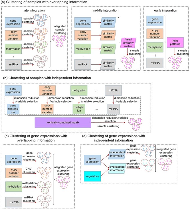
Illustration of unsupervised joint vertical integration approaches taking advantage of overlapping and independent information, respectively. CNV stands for copy number variation.

The first category contains the late integration methods mainly based on the consensus clustering techniques, such as the assisted weighted normalized cut (AWNCut) approach [35], multi-view genomic data integration (MVDA) approach [36], Bayesian consensus clustering (BayesianCC) [37], integrative context-dependent clustering (Clusternomics) [38] and Bayesian two-way latent structure model (BayesianTWL) [39]. These methods differ in the base clustering techniques, ways for extracting useful gene expression/regulator information and some other aspects. Here we use the AWNCut as an example to provide some insights into the strategy [35]. Denote as the number of independent samples. First consider the ‘standard’ NCut analysis. Compute the adjacency matrices and , which measure the ‘closeness’ of any two samples based on gene expressions and regulators, respectively. A simple choice is the inverse of the Euclidean distance. Denote as the number of sample clusters and as their index sets. Using gene expression data only, the NCut approach maximizes the objective function:

(1)

where is the complement of , measures the within-cluster similarity and measures the across-cluster similarity. With the consideration that not all genes/regulators are equally informative, the AWNCut approach first introduces weights—genes/regulators with higher weights are more informative for clustering. Denote and as the weighted counterparts of and , respectively. The AWNCut approach maximizes the objective function:

(2)

where and are two data-dependent tuning parameters and can be selected, for example, using cross validation. and are the th components of the unknown weights for and , respectively. measures the average correlation between the th component of and , computed using samples in , and is defined similarly. It is noted that the clustering structure and weights are optimized simultaneously.

The following observations can be made with this approach and are also applicable to several other consensus clustering methods. First, the key clustering strategy and most important component—the objective function—are built on an existing single-data-type approach (in this case NCut). Second, clusterings are conducted separately using gene expressions and regulators, and consensus is fully reinforced or encouraged. Third, certain mechanisms are needed to remove noises so as to conduct clustering using only informative genes/regulators. With AWNCut, data-dependent weights are imposed, and thresholding can be employed to distinguish signals from noises. With some approaches, regularization has been directly employed for such a purpose.

The second category contains the middle integration methods, which take advantage of similarity-based analysis, including the similarity network fusion (SNF) approach [40] and some others [41–43]. In particular, these methods first build similarity matrices of samples using gene expressions and regulators separately, which are often represented as graphs or networks. Fusion techniques, from as simple as average for PINS [41] and NEMO [42] to the more complex Eigen-decomposition based for CoALa [43], are applied to these similarity matrices to generate a single combined similarity matrix, which is then partitioned using a conventional clustering method, such as the spectral or k-means clustering. Different from the late integration methods which directly generate cluster memberships for gene expressions and regulators separately, followed by a post hoc integration of these separate clusterings, middle integration conducts integration for similarity matrices in an earlier step.

The third category contains the early integration methods, which first detect joint patterns (overlapping information) across gene expressions and regulators and then build a single clustering model that accounts for the generated overlapping information. In a sense, the integration is earlier than the aforementioned ones. These methods are mainly based on the joint dimension reduction techniques, among which iCluster [44, 45] is perhaps the most representative. The basic formulation of iCluster is

(3)

where is the latent component that connects gene expressions and regulators and induces their dependencies; and are independent ‘errors’ for gene expressions and regulators, respectively; and and are the coefficient matrices. The objective function is built on the Gaussian distribution assumption with , and To accommodate high dimensionality and identify informative genes and regulators, the Lasso penalty is imposed on and . An EM algorithm is applied for optimization, and cluster memberships are then assigned by applying a standard k-means clustering on the posterior mean . Similar to in late integration, regularization is usually employed for sparse estimation. Other examples include iClusterPlus [46], LRAcluster [47], moCluster [48], GST-iCluster [49], iClusterBayes [50], MOFA [51] and others.

Complementary to the first strategy, the second strategy has been developed to take advantage of the independent information in gene expressions and regulators [52–54]. As a representative example, a recent approach DLMI [54] is based on modern deep learning techniques and proceeds as follows: (a) gene expression and regulator data are stacked together and then used as the input of an autoencoder which is an unsupervised, feed-forward and nonrecurrent neural network (NN); (b) the output of the NN produces new features, which are nonlinear combinations of the original measurements; (c) to make the analysis clinically more relevant, an outcome variable is used for supervised screening and identify marginally important features from Step (b); and (d) the selected features are used to cluster samples with the k-means approach. With this approach, gene expressions and regulators are explicitly pooled in Step (a) to gain more information. This approach is also a good showcase of data integration in the modern deep learning era.

Clustering gene expressions

Our limited literature review suggests that, compared to the analysis described in the above subsection, gene expression clustering that integrates regulator data is limited. The graphical presentation is also provided in Figure 1.

To take advantage of the overlapping information, we conjecture that it is possible to proceed as follows: (a) for each gene expression, identify its regulators; (b) for a partition of gene expressions, compute the ordinary within-cluster and across-cluster distances; (c) partition regulators based on their associations with gene expressions and the partition in (b). Note that a regulator may belong to multiple clusters. Compute the within-cluster and across-cluster distances, and (d) compute the (weighted) sums of within-cluster and across-cluster distances from (b) and (c), and determine the clustering structure by minimizing the within-cluster distance and maximizing the across-cluster distance. This conjectured approach has been motivated by AWNCut, although we note that it has not been actually executed. And we have not been able to identify a clustering approach motivated by the overlapping information.

To take advantage of the independent information, we consider the ANCut (assisted NCut) approach [55], which is also built on the NCut technique and proceeds as follows. First consider the model

(4)

where is the matrix of unknown regression coefficients, and is the vector of ‘random errors’ (which may also contain unmeasured or unknown regulating mechanisms). In [55], the estimate of is obtained using the elastic net approach, which can accommodate the sparsity of regulations. Denote and . Here a linear regression is adopted to explicitly describe that gene expression data contain information overlapping with regulator data (that is, ) as well as independent information (that is, ). Denote and as the sample adjacency matrices computed using and , respectively. Denote as the number of gene clusters and as their index sets. The ANCut objective function is

(5)

A simplified version, which is suggested as equivalent, has also been developed [55]. The essence of this approach is to first decompose gene expressions into two components and then reinforce that they generate the same clustering results.

Remarks

The aforementioned clustering techniques generate disjoint clusters. In the clustering of samples, clustering of gene expressions and biclustering, fuzzy techniques [56–59] have been developed to allow samples/genes to belong to multiple clusters or not be clustered. Data integration in fuzzy clustering remains limited and may warrant more exploration.

Supervised analysis with sparsity

For a specific outcome/response, it is usually true that many or most genes are ‘noises’, demanding certain sparsity in analysis. Sparse results are also more interpretable and more actionable. The strategies of the supervised integration approaches are illustrated in Figure 2.

Figure 2 .

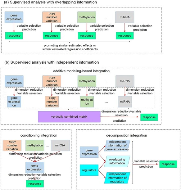
Illustration of supervised joint vertical integration approaches taking advantage of overlapping and independent information, respectively.

Analysis that takes advantage of the overlapping information

A well-known representative is collaborative regression (CollRe) [60], which is motivated by the unit–rank canonical correlation analysis. Consider the case with a continuous and the model , where is the vector of unknown regression coefficients and is the random error. Use subscript to denote the th sample. With the Lasso estimation, the objective function is

(6)

where is the data-dependent tuning parameter and the norm is defined as the sum of component-wise absolute values. Following the same strategy, a model can be built using the regulators, and denote the corresponding regression coefficient vector as . The collaborative regression approach considers the objective function:

(7)

where is another data-dependent tuning parameter. This approach explicitly builds two regression models. The key advancement is the last penalty term, which encourages gene expressions and regulators to generate similar estimated effects.

Motivated by the successes of approaches that explicitly model the gene–regulator relationship and possible long-tailed distribution/contamination of the response data, the ARMI (assisted robust marker identification) approach is developed [61]. Specifically, still consider the linear gene expression–regulator model as in Section Clustering gene expressions. In [61], is obtained using the Lasso approach. The ARMI approach has objective function:

(8)

Different from collaborative regression, it promotes the similarity of regression coefficients for gene expressions and regulators, as opposed to the estimated effects. In addition, the loss functions are adopted, which leads to robustness and simplified computation (as all terms are ).

Remarks: With both collaborative regression and ARMI, the goodness-of-fit functions can be replaced by negative likelihood functions to accommodate other models and data distributions. For example, a follow-up study [62] extends collaborative regression and develops canonical variate regression (CVR) which can handle multivariate and noncontinuous outcomes and allows for multiple-rank modeling. For these two approaches and those described below, the original publications have assumed homogeneity. We conjecture that they can be extended and coupled with the FMR (finite mixture of regression) technique [63, 64] to accommodate heterogeneity. In addition, they have been described with only the additive effects of omics measurements. In practical data analysis, demographic/clinical/environmental variables, which are usually low-dimensional, can be easily incorporated. We conjecture that it is possible to extend the approaches aforementioned and below to accommodate gene–environment interactions [65, 66], although our literature search shows that this has not been pursued.

Analysis that takes advantage of the independent information

Conceptually, the most straightforward approach is to pool all omics measurements together and use as input to, for example, penalization estimation and variable selection. As different types of omics data have significantly different dimensionalities and distributional properties, this simple approach barely works in practical data analysis. To tackle this problem, IPF-LASSO proposes using different penalty parameters for different types of predictors [67]. As an ‘upgrade’, the additive modeling approach first applies, for example, Lasso to each type of omics data separately and identifies a small number of features [68, 69]. The selected features, which have much lower dimensions, are pooled and modeled in an additive manner. The most significant advantage of this approach is simplicity. On the other hand, there is no distinction between gene expressions and regulators.

The conditioning–integration approach has been designed to account for the ‘order’ of omics measurements. That is, compared to regulators, gene expressions are ‘closer to’ outcome/response. This approach proceeds as follows: (a) conduct analysis with gene expression data only, using a ‘standard’ high-dimensional sparse approach, for example, Lasso. With this step, the dimensionality of gene expressions is reduced to one; (b) conditional on the one-dimensional gene expression effect, integrate one type of regulator data. This can be achieved using the same approach as in (a); (c) conduct (b) with all types of regulator data (if applicable), and select the type with, for example, the best prediction performance, and integrate; (d) repeat (c) until there is no significant improvement in prediction or all regulator data have been integrated. A significant advantage of this approach is that it does not demand new methodological and computational development. It can also generate a ‘ranking’ of regulator data, facilitating biological interpretations. On the other hand, it does not take full advantage of the regulation relationship.

Overlapping information may be statistically manifested as correlation, which may challenge model estimation. The decomposition–integration approach explicitly exploits the regulation relationship and can effectively eliminate correlation. A representative example is the LRM-SVD approach [34], which proceeds as follows: (a) consider the regulation model , and denote as the estimate of . In [34], estimation is achieved using Lasso. (b) Conduct sparse SVD (singular value decomposition) with . Specifically, the first step is conducted by minimizing the objective function:

(10)

where is the first singular value, and and are singular vectors with the same dimensions as and , respectively. is then updated, and the subsequent steps can be conducted in a similar manner. (c) With each sparse SVD, Step (b) leads to rank-one subspaces of and (which are linear combinations of a few components of and , corresponding to the nonzero components of the singular vectors). These rank-one subspaces have been referred to as the ‘linear regulatory modules (LRMs)’ and include co-expressed gene expressions and their coordinated regulators. Denote the collection of such subspaces as . (d) Project and onto , and denote the ‘residuals’ as and . This is realized using matrix projection operations. (e) Consider the outcome model . In [34], survival data and the accelerated failure time model are considered. Denote as the lack-of-fit function. The final estimation and variable selection can be achieved by minimizing

(11)

The three decomposed components have lucid interpretations. The LRMs, besides serving as the building blocks for model fitting, can also facilitate understanding biology. In addition, through projection, the three components are statistically independent, facilitating estimation.

Supervised analysis without sparsity

The approaches reviewed in Section Supervised analysis with sparsity and those alike make the sparsity assumption. In practical data analysis, they usually select only a few gene expressions (and regulators). It has been proposed that there may be many weak signals, which cannot be accommodated by sparse approaches. When biological interpretation is of secondary concern, dense approaches that can accommodate many genes may be advantageous. Studies have suggested that some ‘black box’ approaches may excel in prediction.

With the additive modeling and conditioning–integration techniques discussed in Section Supervised analysis with sparsity, dense dimension reduction approaches, such as PCA (principle component analysis), PLS (partial least squares), ICA (independent component analysis) and SIR (slice inverse regression), can be applied as building blocks to accommodate high dimensionality [6]. Examining the decomposition–integration technique suggests that it is designed to be sparse. We have not identified a dense approach that adopts this technique.

In recent studies, deep learning techniques have also been adopted for supervised model building and prediction. Here we note that for data with low-dimensional input and a large number of training samples, the superiority of deep learning in prediction has been well demonstrated. However, the message is less clear with high-dimensional omics data. As a representative, a recent deep learning approach HI-DFNForest [70] proceeds as follows: (a) for gene expression and each type of regulator, data representations are learned separately. This can be achieved using fully connected NNs, although our personal observation is that those with regularization (e.g. Lasso) may be more reliable. (b) All the learned representations are integrated into a layer of autoencoder to learn more complex representations. (c) The learned representations from (b) are fed into another NN for the outcome/phenotype. For continuous, categorical and censored survival outcomes, NNs with various complexity levels have been developed in the recent literature, including MVFA [71], SALMON [72], MDNNMD [73] and others.

Remarks

The line between sparse and dense approaches is becoming blurry. Hybrid approaches have been developed, with the hope to ‘inherit’ strengths from both families of approaches. For example, in a study of the gene expression–regulator relationship [74], a sparse canonical correlation analysis approach is developed, which applies the Lasso penalization to correlation analysis. Other examples include the joint and individual variation explained method [75] and penalized co-inertia analysis [76]. In supervised model building, the SPCA (sparse PCA) and SPLS (sparse PLS) techniques have been applied [69, 77].

Discussions

Methodological notes

Most of the reviewed approaches, for example, AWNCut, collaborative regression, conditioning–integration and many alike in published literature, have roots deep in the existing methods for gene expression only. There are only a few, such as the decomposition–integration approach, that directly take a system perspective. More developments are needed to directly start with the gene expression–regulator system.

Most of the reviewed approaches have been based on penalized variable selection and dimension reduction, which are arguably the most popular high-dimensional techniques. There have also been developments using other techniques, especially including Bayesian, thresholding and boosting. For example, the iBAG approach [78], which adopts the decomposition–integration strategy, has been developed using the Bayesian technique. With the complexity of omics data, it is unlikely that one technique can beat all. It is of interest to expand the aforementioned studies using alternative techniques and comprehensively compare (e.g. consensus clustering using the NCut technique against k-means).

It is indisputable that regulator data contain valuable information. However, in any statistical analysis with a fixed sample size, regulator data contain both signals (which are unknown and need to be identified data-dependently) and noises. Conceptually, if signals overweigh noises, then data integration is worthwhile. However, theoretically, there is still a lack of research on the sufficient (and possibly also necessary) conditions under which data integration is beneficial. We conjecture that this is related to the level of signals, number/ratio of signals and analysis techniques. There have been a few studies conducting numerical comparisons. For example, in [6], with survival data, the models with gene expression only are compared against those integrating regulators including copy number variation, methylation and miRNA using C-statistics. Conflicting observations are made across diseases/datasets, further demonstrating the necessity of more statistical investigations on the benefit of data integration.

The reviewed approaches and many in the literature focus on gene expressions and their upstream regulators. In the whole molecular system, there are also proteomic and metabolic measurements. It is possible to further expand the scope of data integration. One possibility is to keep the central role of gene expressions and use downstream data to assist gene expression analysis. For example, multiple studies have used protein–protein interaction information in gene expression data analysis [79, 80]. The second possibility is to consider gene expression as an intermediate step and directly model the whole system. For example, in [81], clustering analysis (MuNCut) is conducted on the ‘protein-gene expression–regulator’ system and identifies molecular channels.

Our review has been focused on bulk gene expression data, where, for a specific gene, the measurement is the average of transcription levels within a cell population collected from a biological sample. In the past few years, single cell RNA sequencing (scRNA-seq) is getting increasingly popular. It advances from bulk RNA-seq by measuring mRNA expressions in individual cells and can provide more comprehensive understanding of complex heterogeneous tissues, dynamic biological processes and other aspects [82]. Parallel single cell sequencing techniques have also been developed for the joint profiling of single cell transcriptome and other molecular layers, such as genome [83], DNA methylation [84] and chromatin accessibility [85], on the same cells, making it potentially possible to conduct data integration at the single cell resolution [86]. Single cell data usually has the count nature and exhibit strong amplification biases, dropouts and batch effects due to unwanted technical effects, tiny amount of RNA present in a single cell and other reasons [87], posing tremendous challenges to statistical analysis. The integration approaches reviewed above do not account for these characteristics and cannot be applied to single cell data directly. We conjecture that it is possible to build the single cell counterparts of the review methods. However, significant methodological developments will be needed. The limited existing vertical integration approaches for single cell data include the coupled nonnegative matrix factorization for the clustering of cells [88], multi-omics factor analysis v2 (MOFA+) [89] which is the extension of the unsupervised sample clustering approach MOFA [51] and a few others.

Computational notes

In data integration, higher dimensionality inevitably brings computational challenges. This is multifaceted. First, it increases data storage and manipulation burden. This can be especially true when, for example, genome-wide SNP data is present. In practical data analysis, preprocessing is usually conducted to significantly reduce dimensionality and hence computational challenges. For example, SNP data can be aggregated to gene-level data [90], or supervised screening can be applied to select the most relevant ones for downstream analysis [6, 34, 69]. This way, the increase in storage and manipulation burden can be moderate. Second, some methods demand the development of new computational algorithms. For example, AWNCut introduces weights, which need to be optimized along with cluster memberships. The decomposition–integration approach LRM-SVD demands a more effective way of conducting sparse SVD. Fortunately, in the reviewed studies, computational algorithms have been developed by ‘combining’ existing techniques. For example, with AWNCut, the simulated annealing technique is repeatedly applied. Deep learning-based integration approaches have taken advantage of the existing algorithms/tools, such as the Keras library [54], TensorFlow [73] and others. Overall, the demand for new computational algorithms has been ‘affordable’. Third, increased dimensionality reduces computational stability. In some studies [35], random-splitting approaches have been applied to evaluate stability. However, there is still a lack of study rigorously quantifying the loss of stability and whether that can be ‘compensated’ by, for example, the improvement in prediction.

Software developments

Computer programs and packages accompanying some of the published studies have been made publicly available, although in general, our observation is that there is still significant need for more software development. In Table 2, we summarize the publicly available computer programs for the aforementioned approaches, including their types/realized languages and corresponding websites. Specifically, some programs have been made available at the developers’ websites. For example, both R and Matlab codes for SNF [40], a clustering approach via data integration, are available at http://compbio.cs.toronto.edu/SNF/SNF/Software.html, and the R codes for iPF (integrative phenotyping framework) [52] and IS-Kmeans (integrative sparse K-means) [53], both of which conduct unsupervised sample clustering analysis utilizing independent information, are available at Prof. George Tseng’s website http://tsenglab.biostat.pitt.edu/software.htm. Some programs are available at public repositories. For example, the AWNCut [35] and ANCut [55] (along with a few other clustering methods) are available at CRAN (https://cran.r-project.org/web/packages/NCutYX/), and the iBAG code [78] is available at GitHub (https://github.com/umich-biostatistics/iBAG). Computer programs, usually in Python, for some deep learning approaches have also been available at GitHub. Some studies [43, 54] have not provided explicit information on software availability.

Table 2.

Summary of software and application of vertical integration approaches (partial list)

Approach	Software typea	Software website	Applicationb
Unsupervised analysis
AWNCut [35],	R package	https://cran.r-project.org/web/packages/NCutYX	GE, CNV
ANCut [55],			GE, CNV
MuNCut [81]			Protein, GE, CNV
MVDA [36]	R package	https://github.com/angy89/MVDA_package	(1) GE, miRNA; (2) Protein, GE, miRNA; (3) GE, miRNA, CNV
BayesianCC [37]	R package	https://github.com/david-dunson/bayesCC	Protein, GE, miRNA, ME
Clusternomics [38]	R package	https://github.com/evelinag/clusternomics	Protein, GE, miRNA, ME
BayesianTWL [39]	R package	https://cran.r-project.org/web/packages/twl	GE, CNV, ME
SNF [40]	R and Matlab codes	http://compbio.cs.toronto.edu/SNF/SNF/Software.html	GE, miRNA, ME
PINS [41]	R package	https://cran.r-project.org/web/packages/PINSPlus/	GE, miRNA, ME
NEMO [42]	R package	https://github.com/Shamir-Lab/NEMO	GE, miRNA, ME
CoALa [43]	–	–	Protein, GE, miRNA, ME
iCluster [44, 45],	R package	http://www.bioconductor.org/packages/devel/bioc/html/iClusterPlus.html	(1) GE, CNV; (2) GE, ME
iClusterPlus [46],			(1) GE, CNV, mutation; (2) GE, CNV, ME
iClusterBayes [50]			(1) GE, CNV, mutation; (2) GE, CNV, ME, miRNA, mutation
LRAcluster [47]	R code	http://bioinfo.au.tsinghua.edu.cn/software/lracluster	GE, CNV, ME, mutation
MoCluster [48]	R package	https://www.bioconductor.org/packages/release/bioc/html/mogsa.html	(1) Protein, GE; (2) Protein, GE, ME
MOFA [51]	R package	https://bioconductor.org/packages/devel/bioc/html/MOFA.html	GE, ME, mutation
GST-iCluster [49],	R code	http://tsenglab.biostat.pitt.edu/software.htm	(1) GE, CNV, ME; (2) GE, miRNA
IPF [52],			GE, miRNA, Clinical
IS-Kmeans [53]			(1) GE, CNV, ME; (2) GE, CNV
Supervised analysis
DLMI [54]	–	–	GE, miRNA, ME
CollRe [60]	–	–	GE, CNV
ARMI [61]	R code	https://github.com/shuanggema/ARMI	GE, CNV
CVR [62]	R package	https://cran.r-project.org/web/packages/CVR	GE, ME
IPF-LASSO [67]	R package	https://cran.r-project.org/web/packages/ipflasso	GE, CNV, Clinical
IntCox-OV [68]	–	–	GE, CNV, miRNA, ME
IntCox-SKCM [69]	–	–	GE, CNV, ME, mutation, Clinical
LRM-SVD [34]	–	–	GE, CNV, ME
HI-DFNForest [70]	–	–	GE, miRNA, ME
MVFA [71]	Python code	https://github.com/BeautyOfWeb/Multiview-AutoEncoder	Protein, GE, miRNA, ME
SALMON [72]	Python code	https://github.com/huangzhii/SALMON	GE, CNV, miRNA, mutation, Clinical
MDNNMD [73]	Python code	https://github.com/USTC-HIlab/MDNNMD	GE, CNV, Clinical
iBAG [78]	R code	https://github.com/umich-biostatistics/iBAG	GE, ME, Clinical

^aThe type ‘R package’ means that the package can be installed in R via, for example, ‘install_github’, ‘install.packages’ or ‘BiocManager::install’.

^bGE, CNV, ME and Clinical stand for mRNA gene expressions, copy number variations, DNA methylation and clinical features, respectively.

Numerical performance

It is a prohibitive task to implement all the reviewed approaches to conduct rigorous numerical comparisons. As an alternative, we briefly review the existing numerical results reported in some of the published articles, which may provide some insights into numerical performance of the reviewed approaches. Specifically, we summarize the simulation settings and/or analyzed practical data as well as main conclusions in Table 3. It is observed that performance of the approaches depends on the data generation mechanisms (including, e.g. the sample size, data dimensionality, number of clusters, underlying models to describe regulation relationships and others), and no approach can have significant superiority under all scenarios.

Table 3.

Summary of comparisons of vertical integration approaches (partial list)

Reference	Proposed/alternatives	Main settings or datasets	Major observations
Unsupervised analysis: simulated data
Gabasova et al. [38]	Clusternomics/BayesianCC, iCluster, SNF	A mixture probability is first generated from . For the first group of 100 samples, each of the two context values is generated independently from or with probability and . For the next group of 100 samples, each of the two context values is generated independently from or with probability and , respectively.	For small values of , which correspond to two fully dependent global clusters, Clusternomics and BayesianCC perform much better than iCluster and SNF which use k-means and spectral clustering to extract the number of clusters, leading to high sensitivity to mis-specification. For larger values of , which represent higher degrees of independence of clusters between contexts, Clusternomics and iCluster have the best performance. In addition, change of the cluster number does not affect Clusternomics and BayesianCC, but iCluster and SNF are strongly dependent on this setting.
Kim et al. [49]	GST-iCluster/iCluster	There are two types of data, and each data contains three true sample clusters and five gene clusters. The size of sample cluster is generated from a Poisson distribution. Values of predictors are generated from multivariate Normal distributions. The numbers of predictors are 500 and 1500, among which 50 and 150 are important. In each gene cluster, there are five feature modules which reflect across omics regulatory information.	GST-iCluster shows improved clustering accuracy, particularly when a small number of features are used for clustering, due to the incorporation of prior module knowledge. GST-iCluster can find more module genes than iCluster. In addition, when there exist noisy features in the modules, performance of GST-iCluster decays, but is still better than iCluster.
Argelaguet et al. [51]	MOFA/iCluster	Data are generated from the generative model with a varying number of data types (), features (), important factors , missing values (from to ) as well as from non-Gaussian distributions (Poisson and Bernoulli).	MOFA is able to accurately reconstruct the latent dimension, except in settings with a large number of factors or high proportion of missing values. iCluster tends to infer redundant factors and is less accurate in recovering the patterns of shared factor activity across data types. MOFA is also computationally more efficient than iCluster. Take the CLL data as an example. MOFA and iCluster take about 25 min and 5–6 days, respectively.
Unsupervised analysis: real data
Nguyen et al. [41]	PINS/iClusterPlus, SNF	Six TCGA datasets, including KIRC, GBM, LAML, LUSC, BRCA and COAD, with mRNA gene expression, DNA methylation and miRNA expression measurements.	PINS identifies subgroups that have statistically significant differences in survival for all six cancer types, except for COAD. However, SNF and iClusterPlus find significant subgroups only for LAML. PINS needs a significantly longer time than SNF to perform analysis on larger datasets.
Rappoport et al. [42]	NEMO/LARcluster, PINS, SNF, iClusterBayes	Ten TCGA datasets, including LAML, BRCA, COAD, GBM, KIRC, LIHC, LUSC, SKCM, OV and SARC, with mRNA gene expression, DNA methylation and miRNA expression measurements.	NEMO finds clustering with significant difference in survival for 6 out of 10 cancer types, while the other methods find at most 5 (LRAcluster, 5; PINS, 5; SNF, 4; iClusterBayes, 2). None of the methods finds clustering with significantly different survival for COAD, LUSC and OV. NEMO has the fastest average runtime. All methods except for LRAcluster and iClusterBayes take only a few minutes to run on datasets with hundreds of samples and tens of thousands of features.
Khan et al. [43]	CoALa/LARcluster, iCluster, SNF	Four TCGA datasets, including COAD, GBM, STAD and BRCA, with protein expression, mRNA gene expression, DNA methylation and miRNA expression measurements.	CoALa performs better than the alternatives for COAD, GBM and STAD in terms of clustering accuracy. iCluster has comparable performance for BRCA and COAD but degraded performance for the remaining datasets. In terms of the compactness and separability of the clusters, CoALa has the best performance in terms of the Silhouette, DB and Xie-Beni indices for GBM and the second best in terms of the Silhouette and Dunn indices for BRCA, and SNF has the best performance in terms of two or more indices for COAD, STAD and BRCA. CoALa is computationally much faster than LRAcluster and iCluster but slower than SNF.
Wu et al. [47]	LRAcluster/iClusterPlus	Three TCGA datasets, including BRCA, COAD and LUAD, with mRNA gene expression and DNA methylation measurements.	Both LRAcluster and iClusterPlus have high classification accuracy for the three cancer types in the reduced low-dimension subspaces. The clustering performance of LRAcluster is superior to iClusterPlus, especially when the target dimension is large, indicating that iClusterPlus will encounter local optimal problems when the model becomes complex, while the convexity of the LRAcluster model ensures stable model fitting. LRAcluster runs ~5 fold faster than iClusterPlus with a fixed penalty parameter and much faster (~300-fold) if that parameter is optimized.
Supervised analysis: simulated data
Zhu et al. [34]	LRM-SVD/Lasso-Joint, CollRe	There are two types of data, where the regulators are generated from multivariate Normal distributions, and gene expressions are generated via a linear model to reflect across omics regulation. For the response, four scenarios, which represent different levels of complexity of LRMs and individual effects, are considered.	LRM-SVD has higher PAUCs than CollRe for both GE and regulator selection. Lasso-Joint usually performs the worst. CollRe is often the second best. However, some individual variables can be missed due to the mismatch of the two spaces since the individual gene expression signals cannot be explained by the individual regulator signals.
Chai et al. [61]	ARMI/Lasso-Joint, CollRe	Three simulation settings are considered, with multiple scenarios under each setting. Under Settings I and II, there is one type of regulator, and the effects of regulators on outcome are completely captured by gene expressions (GEs), and GEs do not have ‘unregulated effects’ under Setting I, and GEs and regulators have overlapping effects as well as independent effects under Setting II. Under Setting III, there are two types of regulators, and one type of regulator is regulated by the other.	ARMI has competitive performance across the whole spectrum of simulation, even under setting II with a moderate model mis-specification. Lasso-Joint and CollRe have inferior performance without explicitly accounting for the regulation relationship, although they also jointly analyze GEs and regulators and borrow information.

For example, as reported in [38], compared to iCluster, BayesianCC performs much better when there is a common shared clustering structure, but worse when there are higher degrees of independence of clusters. Even with the same data, an approach may have different performance possibly because of differences in preprocessing and other reasons. For example, the TCGA LUSC data are analyzed in two studies [41,42] with PINS. PINS is observed to be able to identify subgroups with statistically significant difference in survival in one study [41] but loses effectiveness in the other [42]. Computational efficiency is also examined in some papers. For example, it is observed that, among the unsupervised analysis approaches, SNF is computationally more efficient, while iCluster, iClusterPlus and iClusterBayes are more expensive.

Application notes

Prior to analysis, data processing is usually needed. Consider a representative example [6], where data processing includes the following steps. (a) Quality control and normalization are conducted with each type of omics data separately. Best practice should be adopted, while consistency across data types is desired. (b) Missing data are accommodated for each data type separately, for example, using multiple imputations. The approaches reviewed above usually do not have built-in mechanisms to accommodate missingness. (c) Unsupervised screening is conducted for quality control purposes. (d) Supervised screening is conducted to screen out noises, improve computational performance and change dimensionalities to more comparable. (e) Finally, merge multiple types of data based on sample IDs.

In the aforementioned studies, one popular (or possibly the most popular) data source is TCGA, because of its high-quality and public availability. TCGA data contain measurements on gene expression, protein expression, methylation, SNP, copy number variation, miRNA and others. This level of comprehensiveness is uniquely valuable. There are other ‘scattered’ public databases. For example, one recent study [77] analyzes data with gene expression and copy number variation measurements on mental disorders collected by the Stanley Medical Research Institute. There are also studies that analyze ‘private’ data generated in individual labs [44, 52, 60]. The aforementioned approaches have been applied to the analysis of different combinations of omics data, which is also summarized in Table 2. Some studies integrate gene expression with only one type of regulator, and popular choices are copy number variation [35, 60] and methylation [62, 78]. There are also studies that integrate multiple types of regulators, including methylation, copy number variation, miRNA and mutation, where different types of regulators are treated separately and equally in most studies [36, 40] or combined into a mega regulator vector in a few others [34, 61]. In addition, besides gene expressions and regulators, protein expressions have also been jointly analyzed in the literature [37, 38]. Our examination suggests that the reviewed and many other integration approaches can be directly applied to other combinations of omics data.

As partly discussed above, theoretical studies on data integration have been limited. Simulation has been extensively conducted. Our observations and recommendations are as follows. First, multiple scenarios on the role of regulator data should be examined, especially including their interconnections with gene expressions (overlapping information) and contributions to outcomes (independent information). The first aspect can be achieved by, for example, varying the sparsity and magnitude of in the gene expression–regulator model. And the second aspect can be achieved by, for example, varying the coefficients of in the decomposition–integration approach. Second, gene expression-only and earlier data integration approaches should be considered as benchmark. For example, in the ARMI study [61], gene expression-only analysis, naïve additive modeling, marginal analysis and collaborative regression are considered for comparison. Third, it should be realized that simulated data based on simple distributions/models are often overly simplified. As such, practical data-based simulation is recommended [35, 77], which can maintain distributional and regulation properties.

Data described above and others have been analyzed, showing that integration can lead to biologically sensible and statistically satisfactory results. For example, ANCut [55] has been applied to the analysis of TCGA SKCM (skin cutaneous melanoma) data, with 382 gene expression and corresponding copy number variation measurements on 366 samples. It is found that ANCut generates more ‘balanced’ clusters (with sizes 110, 105, 97 and 70), compared to the highly unbalanced k-means clusters (with sizes 27, 350, 1 and 4). Bioinformatics analysis is further conducted by examining the GO biological processes, and it is found that the ANCut clusters are enriched with certain well-defined processes (as such, the results are interpretable). As another example, the TCGA LUAD (lung adenocarcinoma) data have been analyzed using the ARMI approach [61]. In this analysis, FEV1, a biomarker for lung capacity and prognostic for lung cancer, is analyzed as the response. ARMI identifies genes including NOTCH2, BCL2L10, BCL2L2, HDAC3 and others, which have independent evidence of associating with lung cancer and its biomarkers. This provides some support to the biological validity of this approach. A cross-validation based prediction evaluation is conducted, showing that ARMI has a smaller prediction MSE (mean squared error) than the alternatives. In [70], the deep learning approach HI-DFNForest is applied to three TCGA datasets, namely, BRCA, GBM and OV, for subtype classification. HI-DFNForest is observed to have superior classification accuracy compared to the approaches using a single type of data. Take BRCA as an example, the HI-DFNForest approach has the classification accuracy rate 0.846, compared to 0.808, 0.731 and 0.769 with gene expression, methylation and miRNA expression, respectively. We note that, however, promising findings made in the aforementioned studies should be taken cautiously. First, with practical data, there is a lack of gold standard to claim success. Criteria mentioned above are sensible but by no means absolute. Second, some aspects of analysis, for example, stability, have not been well examined. Third, as always, there is a potential ‘publication bias’.

Conclusions

With the growing routineness and reducing cost of profiling, we expect more and more studies that collect data on gene expressions as well as their upstream regulators and downstream products. Studies reviewed in this article and many others in the literature have shown the great potential of data integration for gene expression analysis. In this article, we have conducted a selective review of the existing methods, with the hope to roughly describe the existing framework, some key intuition of their strategies as well as pitfalls and possible new directions. This may assist researchers in the field to more effectively conduct gene expression-based data integration. With our limited knowledge, our selection of analysis methods is inevitably biased. For example, there may be an over-selection of penalized/regularized methods and under-selection of deep learning methods. We have categorized the reviewed approaches based on their mechanisms utilizing the overlapping or independent information. Other categorization strategies have been adopted in the literature, such as the parallel integration (under which different types of omics data are treated equally) and hierarchical/model-based integration (under which the relationships among different omics data types are modeled) [29, 91]. In a sense, these categories are not absolute and may be overlapped with each other. Overall, this study may fill some knowledge gaps and be informative to biomedical researchers.

Mengyun Wu is associate professor in School of Statistics and Management, Shanghai University of Finance and Economics.

Huangdi Yi is a doctoral student in Department of Biostatistics at Yale University.

Shuangge Ma is professor in Department of Biostatistics at Yale University.

Acknowledgements

We thank the editor and reviewers for their careful review and insightful comments, which have led to a significant improvement of this article.

Funding

This work was supported by the National Institutes of Health (CA241699, CA216017); National Science Foundation (1916251); Pilot Award from Yale Cancer Center; Bureau of Statistics of China (2018LD02); ‘Chenguang Program’ supported by Shanghai Education Development Foundation and Shanghai Municipal Education Commission (18CG42); Program for Innovative Research Team of Shanghai University of Finance and Economics; and Shanghai Pujiang Program (19PJ1403600).

References

- 1.Richardson S, Tseng GC, Sun W. Statistical methods in integrative genomics. Annu Rev Stat Appl 2016;3:181–209. [DOI] [PMC free article] [PubMed] [Google Scholar]
- 2.Zhao Q, Shi X, Huang J, et al. Integrative analysis of ‘-omics’ data using penalty functions. WIREs Comput Stat 2015;7(1):99–108. [DOI] [PMC free article] [PubMed] [Google Scholar]
- 3.Huang Y, Zhang Q, Zhang S, et al. Promoting similarity of sparsity structures in integrative analysis with penalization. J Am Stat Assoc 2017;112(517):342–50. [DOI] [PMC free article] [PubMed] [Google Scholar]
- 4.Fang K, Fan X, Zhang Q, et al. Integrative sparse principal component analysis. J Multivariate Anal 2018;166:1–16. [Google Scholar]
- 5.Fan X, Fang K, Ma S, et al. Integrating approximate single factor graphical models. Stat Med 2020;39(2):146–55. [DOI] [PMC free article] [PubMed] [Google Scholar]
- 6.Zhao Q, Shi X, Xie Y, et al. Combining multidimensional genomic measurements for predicting cancer prognosis: observations from TCGA. Brief Bioinform 2014;16(2):291–303. [DOI] [PMC free article] [PubMed] [Google Scholar]
- 7.Karczewski KJ, Snyder MP. Integrative omics for health and disease. Nat Rev Genet 2018;19(5):299–310. [DOI] [PMC free article] [PubMed] [Google Scholar]
- 8.Lin D, Zhang J, Li J, et al. Integrative analysis of multiple diverse omics datasets by sparse group multitask regression. Front Cell Dev Biol 2014;2:62. [DOI] [PMC free article] [PubMed] [Google Scholar]
- 9.Mihaylov I, Kańduła M, Krachunov M, et al. A novel framework for horizontal and vertical data integration in cancer studies with application to survival time prediction models. Biol Direct 2019;14:22. [DOI] [PMC free article] [PubMed] [Google Scholar]
- 10.Park JY, Lock EF. Integrative factorization of bidimensionally linked matrices. Biometrics 2020;76(1):61–74. [DOI] [PMC free article] [PubMed] [Google Scholar]
- 11.Michailidis G. Statistical challenges in biological networks. J Comput Graph Stat 2012;21(4):840–55. [Google Scholar]
- 12.Peterson CB, Stingo FC, Vannucci M. Joint Bayesian variable and graph selection for regression models with network-structured predictors. Stat Med 2016;35(7):1017–31. [DOI] [PMC free article] [PubMed] [Google Scholar]
- 13.Gao B, Liu X, Li H, et al. Integrative analysis of genetical genomics data incorporating network structures. Biometrics 2019;75(4):1063–75. [DOI] [PMC free article] [PubMed] [Google Scholar]
- 14.Wang X, Xu Y, Ma S. Identifying gene-environment interactions incorporating prior information. Stat Med 2019;38(9):1620–33. [DOI] [PMC free article] [PubMed] [Google Scholar]
- 15.Shi X, Zhao Q, Huang J, et al. Deciphering the associations between gene expression and copy number alteration using a sparse double Laplacian shrinkage approach. Bioinformatics 2015;31(24):3977–83. [DOI] [PMC free article] [PubMed] [Google Scholar]
- 16.Wu C, Zhang Q, Jiang Y, et al. Robust network-based analysis of the associations between (epi)genetic measurements. J Multivariate Anal 2018;68:119–30. [DOI] [PMC free article] [PubMed] [Google Scholar]
- 17.Cantini L, Isella C, Petti C, et al. MicroRNA-mRNA interactions underlying colorectal cancer molecular subtypes. Nat Commun 2015;6:8878. [DOI] [PMC free article] [PubMed] [Google Scholar]
- 18.Wang Y, Franks JM, Whitfield ML, et al. BioMethyl: an R package for biological interpretation of DNA methylation data. Bioinformatics 2019;35(19):3635–41. [DOI] [PMC free article] [PubMed] [Google Scholar]
- 19.Shi X, Yi H, Ma S. Measures for the degree of overlap of gene signatures and applications to TCGA. Brief Bioinform 2015;16(5):735–44. [DOI] [PMC free article] [PubMed] [Google Scholar]
- 20.Ma S, Huang J. Penalized feature selection and classification in bioinformatics. Brief Bioinform 2008;9(5):392–403. [DOI] [PMC free article] [PubMed] [Google Scholar]
- 21.Ang JC, Mirzal A, Haron H, et al. Supervised, unsupervised, and semi-supervised feature selection: a review on gene selection. IEEE ACM T Comput BI 2016;13(5):971–89. [DOI] [PubMed] [Google Scholar]
- 22.Gligorijevic V, Malod-Dognin N, PrzUlj N. Integrative methods for analyzing big data in precision medicine. Proteomics 2016;16(5):741–58. [DOI] [PubMed] [Google Scholar]
- 23.Hasin Y, Seldin M, Lusis A. Multi-omics approaches to disease. Genome Biol 2017;18:83. [DOI] [PMC free article] [PubMed] [Google Scholar]
- 24.Chalise P, Koestler DC, Bimali M, et al. Integrative clustering methods for high-dimensional molecular data. Transl Cancer Res 2014;3:202–16. [DOI] [PMC free article] [PubMed] [Google Scholar]
- 25.Wang D, Gu J. Integrative clustering methods of multi-omics data for molecule-based cancer classifications. Quant Biol 2016;4:58–67. [Google Scholar]
- 26.Rappoport N, Shamir R. Multi-omic and multi-view clustering algorithms: review and cancer benchmark. Nucleic Acids Res 2018;46:10546–62. [DOI] [PMC free article] [PubMed] [Google Scholar]
- 27.Tini G, Marchetti L, Priami C, et al. Multi-omics integration-a comparison of unsupervised clustering methodologies. Brief Bioinform 2019;20(4):1269–79. [DOI] [PubMed] [Google Scholar]
- 28.Meng C, Zelezni OA, Thallinger GG, et al. Dimension reduction techniques for the integrative analysis of multi-omics data. Brief Bioinform 2016;17(4):628–41. [DOI] [PMC free article] [PubMed] [Google Scholar]
- 29.Wu C, Zhou F, Ren J, et al. A selective review of multi-level omics data integration using variable selection. High-throughput 2019;8:4. [DOI] [PMC free article] [PubMed] [Google Scholar]
- 30.Mirza B, Wang W, Wang J, et al. Machine learning and integrative analysis of biomedical big data. Gen 2019;10(2):87. [DOI] [PMC free article] [PubMed] [Google Scholar]
- 31.Bersanelli M, Mosca E, Remondini D, et al. Methods for the integration of multi-omics data: mathematical aspects. BMC Bioinform 2016;17(2):15. [DOI] [PMC free article] [PubMed] [Google Scholar]
- 32.Zeng IS, Lumley T. Review of statistical learning methods in integrated omics studies (an integrated information science). Bioinform Biol Insights 2018;12:1–16. [DOI] [PMC free article] [PubMed] [Google Scholar]
- 33.Huang S, Chaudhary K, Garmire LX. More is better: recent progress in multi-omics data integration methods. Front Genet 2017;8:84. [DOI] [PMC free article] [PubMed] [Google Scholar]
- 34.Zhu R, Zhao Q, Zhao H, et al. Integrating multidimensional omics data for cancer outcome. Biostatistics 2016;17(4):605–18. [DOI] [PMC free article] [PubMed] [Google Scholar]
- 35.Li Y, Bie R, Hidalgo SJ, et al. Assisted gene expression-based clustering with AWNCut. Stat Med 2018;37(29):4386–403. [DOI] [PMC free article] [PubMed] [Google Scholar]
- 36.Serra A, Fratello M, Fortino V, et al. MVDA: a multi-view genomic data integration methodology. BMC Bioinform 2015;16:261. [DOI] [PMC free article] [PubMed] [Google Scholar]
- 37.Lock EF, Dunson DB. Bayesian consensus clustering. Bioinformatics 2013;29(20):2610–6. [DOI] [PMC free article] [PubMed] [Google Scholar]
- 38.Gabasova E, Reid JE, Wernisch L. Clusternomics: integrative context-dependent clustering for heterogeneous datasets. PLoS Comput Biol 2017;13(10):e1005781. [DOI] [PMC free article] [PubMed] [Google Scholar]
- 39.Swanson D, Lien TG, Bergholtz H, et al. A Bayesian two-way latent structure model for genomic data integration reveals few pan-genomic cluster subtypes in a breast cancer cohort. Bioinformatics 2019;35(23):4886–97. [DOI] [PubMed] [Google Scholar]
- 40.Wang B, Mezlini AM, Demir F, et al. Similarity network fusion for aggregating data types on a genomic scale. Nat Methods 2014;11(3):333–7. [DOI] [PubMed] [Google Scholar]
- 41.Nguyen T, Tagett R, Diaz D, et al. A novel approach for data integration and disease subtyping. Genome Res 2017;27(12):2025–39. [DOI] [PMC free article] [PubMed] [Google Scholar]
- 42.Rappoport N, Shamir R. NEMO: cancer subtyping by integration of partial multi-omic data. Bioinformatics 2019;35(18):3348–56. [DOI] [PMC free article] [PubMed] [Google Scholar]
- 43.Khan A, Maji P. Approximate graph Laplacians for multimodal data clustering. IEEE T Pattern Anal 2020. doi: 10.1109/TPAMI.2019.2945574. [DOI] [PubMed] [Google Scholar]
- 44.Shen R, Olshen AB, Ladanyi M. Integrative clustering of multiple genomic data types using a joint latent variable model with application to breast and lung cancer subtype analysis. Bioinformatics 2009;25(22):2906–12. [DOI] [PMC free article] [PubMed] [Google Scholar]
- 45.Shen R, Wang S, Mo Q. Sparse integrative clustering of multiple omics data sets. Ann Appl Stat 2013;7(1):269–94. [DOI] [PMC free article] [PubMed] [Google Scholar]
- 46.Mo Q, Wang S, Seshan VE, et al. Pattern discovery and cancer gene identification in integrated cancer genomic data. Proc Nati Acad Sci 2013;110(11):4245–50. [DOI] [PMC free article] [PubMed] [Google Scholar]
- 47.Wu D, Wang D, Zhang MQ, et al. Fast dimension reduction and integrative clustering of multi-omics data using low-rank approximation: application to cancer molecular classification. BMC Genomics 2015;16:1022. [DOI] [PMC free article] [PubMed] [Google Scholar]
- 48.Meng C, Helm D, Frejno M, et al. moCluster: identifying joint patterns across multiple omics datasets. J Proteome Res 2016;15:755–65. [DOI] [PubMed] [Google Scholar]
- 49.Kim S, Oesterreich S, Kim S, et al. Integrative clustering of multi-level omics data for disease subtype discovery using sequential double regularization. Biostatistics 2017;18(1):165–79. [DOI] [PMC free article] [PubMed] [Google Scholar]
- 50.Mo Q, Shen R, Guo C, et al. A fully Bayesian latent variable model for integrative clustering analysis of multi-type omics data. Biostatistics 2018;19(1):71–86. [DOI] [PMC free article] [PubMed] [Google Scholar]
- 51.Argelaguet R, Velten B, Arnol D, et al. Multi-omics factor analysis-a framework for unsupervised integration of multi-omics data sets. Mol Syst Biol 2018;14(6):e8124. [DOI] [PMC free article] [PubMed] [Google Scholar]
- 52.Kim S, Herazomaya JD, Kang DD, et al. Integrative phenotyping framework (iPF): integrative clustering of multiple omics data identifies novel lung disease subphenotypes. BMC Genomics 2015;16:924. [DOI] [PMC free article] [PubMed] [Google Scholar]
- 53.Huo Z, Tseng GC. Integrative sparse K-means with overlapping group lasso in genomic applications for disease subtype discovery. Ann Appl Stat 2017;11(2):1011–39. [DOI] [PMC free article] [PubMed] [Google Scholar]
- 54.Chaudhary K, Poirion OB, Lu L, et al. Deep learning–based multi-omics integration robustly predicts survival in liver cancer. Clin Cancer Res 2018;24(6):1248–59. [DOI] [PMC free article] [PubMed] [Google Scholar]
- 55.Hidalgo SJ, Wu M, Ma S. Assisted clustering of gene expression data using ANCut. BMC Genomics 2017;18:623. [DOI] [PMC free article] [PubMed] [Google Scholar]
- 56.Dembele D, Kastner P. Fuzzy C-means method for clustering microarray data. Bioinformatics 2003;19(8):973–80. [DOI] [PubMed] [Google Scholar]
- 57.Maraziotis IA. A semi-supervised fuzzy clustering algorithm applied to gene expression data. Pattern Recogn 2012;45:637–48. [Google Scholar]
- 58.Hidalgo SJ, Zhu T, Wu M, et al. Overlapping clustering of gene expression data using penalized weighted normalized cut. Genet Epidemiol 2018;42(8):796–811. [DOI] [PMC free article] [PubMed] [Google Scholar]
- 59.Chen L, Yu PS, Tseng VS. WF-MSB: a weighted fuzzy-based biclustering method for gene expression data. Int J Data Min Bioinform 2011;5(1):89–109. [DOI] [PubMed] [Google Scholar]
- 60.Gross SM, Tibshirani R. Collaborative regression. Biostatistics 2015;16(2):326–38. [DOI] [PMC free article] [PubMed] [Google Scholar]
- 61.Chai H, Shi X, Zhang Q, et al. Analysis of cancer gene expression data with an assisted robust marker identification approach. Genet Epidemiol 2017;41(8):779–89. [DOI] [PMC free article] [PubMed] [Google Scholar]
- 62.Luo C, Liu J, Dey DK, et al. Canonical variate regression. Biostatistics 2016;17(3):468–83. [DOI] [PMC free article] [PubMed] [Google Scholar]
- 63.McLachlan GJ, David P. Finite Mixture Models. John Wiley & Sons, 2000. [Google Scholar]
- 64.Liu M, Zhang Q, Fang K, et al. Structured analysis of the high-dimensional FMR model. Comput Stat Data An 2020;144:106883. [DOI] [PMC free article] [PubMed] [Google Scholar]
- 65.Hunter DJ. Gene-environment interactions in human diseases. Nat Rev Genet 2005;6(4):287–98. [DOI] [PubMed] [Google Scholar]
- 66.Wu M, Ma S. Robust genetic interaction analysis. Brief Bioinform 2019;20(2):624–37. [DOI] [PMC free article] [PubMed] [Google Scholar]
- 67.Boulesteix A, De Bin R, Jiang X, et al. IPF-LASSO: integrative L1-penalized regression with penalty factors for prediction based on multi-omics data. Comput Math Method M 2017;7691937. [DOI] [PMC free article] [PubMed] [Google Scholar]
- 68.Mankoo P, Shen R, Schultz N, et al. Time to recurrence and survival in serous ovarian tumors predicted from integrated genomic profiles. PLoS One 2011;6(11):e24709. [DOI] [PMC free article] [PubMed] [Google Scholar]
- 69.Jiang Y, Shi X, Zhao Q, et al. Integrated analysis of multidimensional omics data on cutaneous melanoma prognosis. Genomics 2016;107:223–30. [DOI] [PMC free article] [PubMed] [Google Scholar]
- 70.Xu J, Wu P, Chen Y, et al. A hierarchical integration deep flexible neural forest framework for cancer subtype classification by integrating multi-omics data. BMC Bioinform 2019;20:527. [DOI] [PMC free article] [PubMed] [Google Scholar]
- 71.Ma T, Zhang A. Multi-view factorization autoencoder with network constraints for multi-omic integrative analysis. In: 2018 IEEE International Conference on Bioinformatics and Biomedicine (BIBM) on, Vol. 2018. Spain: Madrid, 2018, 702–7. [Google Scholar]
- 72.Huang Z, Zhan X, Xiang S, et al. SALMON: survival analysis learning with multi-omics neural networks on breast cancer. Front Genet 2019;10:166. [DOI] [PMC free article] [PubMed] [Google Scholar]
- 73.Sun D, Wang M, Li A. A multimodal deep neural network for human breast cancer prognosis prediction by integrating multi-dimensional data. IEEE ACM T Comput BI 2019;16(3):841–50. [DOI] [PubMed] [Google Scholar]
- 74.Witten DM, Tibshirani R, Hastie T. A penalized matrix decomposition, with applications to sparse principal components and canonical correlation analysis. Biostatistics 2009;10(3):515–34. [DOI] [PMC free article] [PubMed] [Google Scholar]
- 75.Lock EF, Hoadley KA, Marron JS, et al. Joint and individual variation explained (JIVE) for integrated analysis of multiple data types. Ann Appl Stat 2013;7:523–42. [DOI] [PMC free article] [PubMed] [Google Scholar]
- 76.Min EJ, Safo SE, Long Q. Penalized co-inertia analysis with applications to omics data. Bioinformatics 2019;35(6):1018–25. [DOI] [PMC free article] [PubMed] [Google Scholar]
- 77.Wang S, Shi X, Wu M, et al. Horizontal and vertical integrative analysis methods for mental disorders omics data. Sci Rep 2019;9:13430. [DOI] [PMC free article] [PubMed] [Google Scholar]
- 78.Wang W, Baladandayuthapani V, Morris JS, et al. IBAG: integrative Bayesian analysis of high-dimensional multiplatform genomics data. Bioinformatics 2013;29(2):149–59. [DOI] [PMC free article] [PubMed] [Google Scholar]
- 79.Wu C, Zhu J, Zhang X. Integrating gene expression and protein-protein interaction network to prioritize cancer-associated genes. BMC Bioinform 2012;13:182. [DOI] [PMC free article] [PubMed] [Google Scholar]
- 80.Kabir H, Patrick R, Ho JW, et al. Identification of active signaling pathways by integrating gene expression and protein interaction data. BMC Syst Biol 2018;12(9):77–87. [DOI] [PMC free article] [PubMed] [Google Scholar]
- 81.Hidalgo SJ, Ma S. Clustering multilayer omics data using MuNCut. BMC Genomics 2018;19:198. [DOI] [PMC free article] [PubMed] [Google Scholar]
- 82.Risso D, Perraudeau F, Gribkova S, et al. A general and flexible method for signal extraction from single-cell RNA-seq data. Nat Commun 2018;9:284. [DOI] [PMC free article] [PubMed] [Google Scholar]
- 83.Macaulay IC, Haerty W, Kumar P, et al. G&T-seq: parallel sequencing of single-cell genomes and transcriptomes. Nat Methods 2015;12:519–22. [DOI] [PubMed] [Google Scholar]
- 84.Angermueller C, Clark SJ, Lee HJ, et al. Parallel single-cell sequencing links transcriptional and epigenetic heterogeneity. Nat Methods 2016;13:229–32. [DOI] [PMC free article] [PubMed] [Google Scholar]
- 85.Cao J, Cusanovich DA, Ramani V, et al. Joint profiling of chromatin accessibility and gene expression in thousands of single cells. Science 2018;361:1380–5. [DOI] [PMC free article] [PubMed] [Google Scholar]
- 86.Stuart T, Satija R. Integrative single-cell analysis. Nat Rev Genet 2019;20:257–72. [DOI] [PubMed] [Google Scholar]
- 87.Petegrosso R, Li Z, Kuang R. Machine learning and statistical methods for clustering single-cell RNA-sequencing data. Brief Bioinform 2020;21:1209–1223. doi: 10.1093/bib/bbz063. [DOI] [PubMed] [Google Scholar]
- 88.Duren Z, Chen X, Zamanighomi M, et al. Integrative analysis of single-cell genomics data by coupled nonnegative matrix factorizations. Proc Natl Acad Sci 2018;115:7723–8. [DOI] [PMC free article] [PubMed] [Google Scholar]
- 89.Argelaguet R, Arnol D, Bredikhin D, et al. MOFA+: a statistical framework for comprehensive integration of multi-modal single-cell data. Genome Biol 2020;21:111. [DOI] [PMC free article] [PubMed] [Google Scholar]
- 90.Yang H, Wang P, Lin C, et al. Integrative analysis of single nucleotide polymorphisms and gene expression efficiently distinguishes samples from closely related ethnic populations. BMC Genomics 2012;13:346. [DOI] [PMC free article] [PubMed] [Google Scholar]
- 91.Liu J, Chen J, Perrone-Bizzozero N, et al. A perspective of the cross-tissue interplay of genetics, epigenetics, and transcriptomics, and their relation to brain based phenotypes in schizophrenia. Front Genet 2018;9:343. [DOI] [PMC free article] [PubMed] [Google Scholar]