Self-selection of evolutionary strategies: adaptive versus non-adaptive forces

Abstract

The evolution of complex genetic networks is shaped over the course of many generations through multiple mechanisms. These mechanisms can be broken into two predominant categories: adaptive forces, such as natural selection, and non-adaptive forces, such as recombination, genetic drift, and random mutation. Adaptive forces are influenced by the environment, where individuals better suited for their ecological niche are more likely to reproduce. This adaptive force results in a selective pressure which creates a bias in the reproduction of individuals with beneficial traits. Non-adaptive forces, in contrast, are not influenced by the environment: Random mutations occur in offspring regardless of whether they improve the fitness of the offspring. Both adaptive and non-adaptive forces play critical roles in the development of a species over time, and both forces are intrinsically linked to one another. We hypothesize that even under a simple sexual reproduction model, selective pressure will result in changes in the mutation rate and genome size. We tested this hypothesis by evolving Boolean networks using a modified genetic algorithm. Our results demonstrate that changes in environmental signals can result in selective pressure which affects mutation rate.

Evolution; Genetic Algorithms; Adaptation.

1. Introduction

Evolution consists of both non-adaptive and adaptive forces. Non-adaptive forces are primarily random, including mutation, genetic drift, and recombination. Adaptive forces depend on the relative or absolute fitness of individuals within a population, such as natural selection. The causes, mechanisms, and outcomes of each of these forces vary. Although all of these forces play critical roles in evolution, mutation is the ultimate source of novel genetic information [1]: recombination utilizes existing genetic material, genetic drift is the stochastic change in allele frequency of existing genes, and natural selection is a bias in the selection of existing organisms because of how existing traits interact with their environment.

Natural selection, mutations, recombination, and genetic drift all interact with one another throughout the course of evolution [2–5]. The interplay between these processes results in the emergence of complex networks of gene interactions, which continue to change over time. Aspects of these networks are gradually changed over the course of generations through both the random and selective pressures of evolution, with beneficial network features more likely to be conserved [3, 4, 6, 7, 8, 9, 10]. The relative influence of each evolutionary force on the formation and modifications of these networks is debated [1, 3, 4, 11, 12], with random, non-adaptive forces limiting the effects of selection under certain circumstances [3, 4, 11, 13].

Some of these forces, such as the rate of mutation, are evolvable traits. The rate of mutation is driven by the fidelity of the DNA replicase which exists within each organism [2, 4, 5, 13, 14]. While the rate of mutation may not affect a living organism's current chance of procreation, mutations that occur during reproduction may be neutral, deleterious, or beneficial. If mutations are more likely to be deleterious, then organisms that have high mutation rates are more likely to have less-fit offspring. It is generally believed that most mutations are neutral, with a small tendency toward deleterious mutations [15, 16]. Under this paradigm most genetic mutations will result in neutral changes to an organism [3, 11]. If neutral forces are the main forces acting on the genetic makeup of a species, then deleterious mutations can only be purged through natural selection if the force of selection is higher than the force of genetic drift [13, 17].

From this we would expect that the evolution of mutation rate would be driven by the selective force against deleterious mutations and the ability of the population to overcome genetic drift, which is determined by population size [4, 13]. Non-adaptive forces, such as drift and random mutations, also play a role in shaping more complex genetic traits, such as genetic regulatory networks [3, 6, 18], and there are a number of different ideas on how function, selection and the non-adaptive processes of evolution influence the formation of these networks [3, 7, 10, 18, 19, 20, 21, 22].

Studying how complex traits, nonadaptive forces, and adaptive forces interact requires a holistic view of the evolutionary process allowing for each respective aspect to properly influence the course of evolution. Proposed models of gene network formation primarily focus on either non-adaptive or adaptive processes as explanations for gene networks, while studies looking into the influence of selective pressure on non-adaptive processes, specifically the effect of selection on mutation rate, are often de-contextualized from more complex polygenic traits.

There has been much research into the paradigm of non-adaptive forces as the primary driver of complex gene network formation, with networks formed by random processes appearing to be similar in structure to biological networks [10, 18, 22, 23]. These non-adaptive network models assert the null hypothesis: The structure of regulatory networks exists because of the rules that create them, not because of the selection of specific functions. These models are proposed as explanations for types of structures found universally within gene networks, such as the scale-free nature of some biological networks [18]. However, other evidence suggests that biological networks may not be scale-free [24, 25] or may not have small world properties [26] and that many functional genetic network structures are conserved over long periods [19, 20, 21]. In addition, these networks present non-adaptive forces (such as mutation rates and gene duplications) as static, constant phenomena when genome size and mutation rate have both been seen to change in response to external stressors [27, 28].

Research into functional network models, focused on the performance of a network rather than the non-adaptive forces that form it, are meant to understand how function influences network structure, and have used a variety of functions models which include electronic logic circuits [8], neural networks [29], and networks that exhibit oscillatory behavior [6, 30]. The algorithms used to identify potential functional network structures are not always evolutionary, which would ignore the influence of non-adaptive processes altogether, and those which are suffer shortfalls by evolving networks using fixed mutation rates [29, 31, 32] or fixed network size [6].

In addition to the non-adaptive network models and functional network models, the third set of relevant models look at the influence of selective pressure on mutation rate. Mutations are the result of a random process, but that random process is a genetically heritable trait which makes it susceptible to the same forces of natural selection. If mutations are generally deleterious then the mutation rate will always be selected against and will asymptotically approach some lower limit, known as the drift barrier hypothesis [4, 13, 17]. Evidence indicates that selective pressure may influence the mutation rate as well, with environmental stressors leading to changes in the mutation rate of a population [2, 5, 12, 33, 34]. The competing ideas of mutation rate being limited by genetic drift, or mutation rate being selected by genetic hitchhiking are not mutually exclusive, with stable populations likely benefiting from a depressed mutation rate while populations in changing environments where multiple beneficial mutations are possible, or even necessary, would be likely to encourage the hitchhiking of higher mutation rate traits. There has been less research which contextualizes the evolution of the mutation rate in the context of complex, polygenic traits.

We propose a computational model of evolution which would allow both adaptive and non-adaptive forces to influence the formation of complex networks, while simultaneously allowing for the mutation rate to act as a heritable trait as it would in real world populations. This model mimics environmental signal transduction to study how environmental pressure, selection of complex traits, and nonadaptive forces interact. The fitness of each individual is determined by how well the evolvable transduction network, represented by a Boolean network, creates a desired output signal based on environmental signals.

This model contextualizes the evolution of mutation rate with the evolution of complex, polygenic traits. We hypothesize that there should be two behaviors of the mutation rate: when the population is relatively stable phenotypically, we should see an asymptotic decrease in the mutation rate, as predicted by the drift-barrier hypothesis, while we would expect drastic changes in the environment to result in increased mutation rate. We can further expect that the mutation rate in these changing environments will generally increase by secondary selection. This would show that while the mutation rate is not tuned to optimize evolution in response to stressors, it still changes in response to stressors and may have broader effects on a population, including increasing genetic diversity.

To capture these behaviors, we performed two types of simulations: one with a static fitness function, and one where the fitness function is changed within a run of the genetic algorithm allowing the same population to evolve in two different epochs. We would expect that the static fitness function populations will have an asymptotically decreasing mutation rate and generally lower diversity over time, while populations which have a change in fitness function will increase their mutation rate when the fitness function changes and as a result have higher diversity.

2. Methods

2.1. Evolutionary algorithm

We used a modified genetic algorithm [35] to simulate the evolution of regulatory networks. These regulatory networks are represented by Boolean networks, with the value of each node being a binary value (0 or 1) at discrete time points represented as integer values. These regulatory networks are simulated multiple times, with each simulation having a stimulatory input signal and different initial conditions for each of the nodes within the network. The network produces an output signal in response to this input and depends on the initial conditions of the network. The fitness of the network depends on how closely the period of the output signal matches the period of the target, summed across the multiple simulations.

For our simulations in this paper there are 3 distinct input signals for each network, with each input signal having a unique target period. The periods of the three targets are linearly related as τ, 2∗τ, and 4∗τ. In these specific simulations τ represents the smallest oscillatory period a network is expected to produce and serves as a normalizing factor to compare how difficult it may be for a population to evolve a specific function. These simulations were performed in two ways: One with a static value of τ for the whole course of the evolution, and one with a τ which changes after a predefined number of generations, which breaks the evolution into two epochs.

In this genetic algorithm an individual I is represented by three parameters: The regulatory network, the mutation rate of the network and the duplication/deletion rate of the network. The regulatory network is the Boolean network discussed briefly above, and in detail below. The mutation rate determines the probability of connections within a network being formed, deleted, or modified. The duplication/deletion rate refers to the probability of a node being duplicated or deleted during the mutation phase of the genetic algorithm. The model is initialized with a population P, which consists of a set of individuals. For our model the population consists of one hundred individuals. Each individual is initially identical: an initial naïve network, a preset mutation rate and a preset duplication/deletion rate. The initial networks have no edges and are hence “naïve”. These networks initially have five nodes, which include one input node, one output node, and three intermediate nodes. The fitness of each individual is assessed, and tournament selection is used to select two individuals (p₁ and p₂) as parents. The parents then generate two offspring o₁ and o₂ by a crossover operator, which results in the new regulatory networks for the next generation.

Each offspring receives the mutation rate and duplication/deletion rate from one of its parents. Each offspring network is mutated based on the inherited mutation rate, and each offspring network has the number of nodes adjusted by the duplication/deletion rate inherited. The mutation rate and duplication/deletion rate are then modified based on a random variable. The offspring replace the parent in the next generation, without any form of ratchet or elitism mechanism. This process is repeated until a predefined number of generations pass. There are no stop conditions based on fitness or other parameters, only based on the number of generations passed. This is summarized by the algorithm (GA) below:

Start GA

initialize P

g = 0

 while g ≤ g_max

 g = g+1

 evaluate fitness of individuals in P

 select parents from individuals in P

 crossover parents to form offspring

 mutate offspring

 duplicate/delete nodes in offspring

 mutate mutation rate and duplication/deletion rates

 end while

end GA

2.1.1. Individual representation

Each individual consists of a regulatory network, a mutation rate, and a duplication/deletion rate. Each regulatory network is modeled using a Boolean network which consists of environmental input, an output, and a series of functional nodes. The regulatory network is represented by an adjacency matrix, which contains all the information necessary to construct the Boolean network. Each row of the matrix represents a node, with each column within that row representing how that node connects to other nodes in the network. For our specific experiments, the first row represents the input node, and the last row represents the output node of the network.

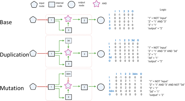
The logic controlling the incoming connections to a node is determined by the numeric values within the adjacency matrix. Each index on the adjacency matrix can have a value of 0, which represents there is no edge present or a positive or negative integer. For example: all incoming edges with a functional value of 1 are combined using an OR function, while all incoming edges with a functional value of 2 are combined using an AND function. Complex functions are then defined by combining multiple functional groups. In the example of Figure 1, the column labelled “2” represents the inputs to Node 2. The presence of 2 inputs each with a value of “2” represents that these inputs will be processed by an AND function. In this way the value of a node N at time point t during the assessment of the regulatory network is determined based on the binary value of the Boolean function associated with that node (B_N) during the prior time point:

$$N\left(t\right)=B_N(t-1)$$

Figure 1.

General overview of how an individual network is processed. Each individual receives an environmental signal. This signal is propagated through the signal processing section of the network and produces an output signal. The network output is used to assess the fitness of the individual. An adjacency matrix expressed the information describing a network. Each row corresponds to a node and each column represents the corresponding connection of that node. The first network describes logic representation. The second network assumed the duplication of node “3” which results in augmenting the logic driving the activity of node “2”. The same node's logic is mutated in the third network. Each index on the adjacency matrix can have a value of 0, which represents there is no edge present or a positive or negative integer. The value represents a logical function associated with the connection: All incoming edges with a functional value of 1 are combined using an OR function, while all incoming edges with a functional value of 2 are combined using an AND function. Complex functions are then defined by combining multiple functional groups. In this example the column labelled “2” represents the inputs to Node 2. The presence of 2 inputs each with a value of “2” represents that these inputs will be processed by an AND function.

The value of each node within the network is either 1 or 0. The functions defining relationships between these nodes are logic functions based on Boolean logic. These functions may be AND, OR, and NOT. Other Boolean functions (such as NAND or XOR) were excluded because they are not generally found in evolved gene networks.

The environmental input is represented by a node in the network (and thus, also represented in the adjacency matrix) whose value is set by the input signal. The network is not allowed to form edges which lead to the input node.

The output is used to measure the fitness of the network and is represented by a node in the network. To prevent any trivial solutions from forming, the output node was not allowed to form any outgoing connections.

Although the input and output nodes have restrictions on having incoming or outgoing edges, there are no restrictions on the other nodes. Because the intermediary nodes have no restrictions, they may form feedback loops, feedforward loops and other networks structures which may create or alter oscillations even if the input is a constant signal.

2.1.2. Fitness evaluation

Each network within a population is assessed for fitness by comparing the output of the network in response to multiple environmental inputs. The simulation of regulatory networks uses k input signals, with each input having a different pattern. This pattern may be a constant (for example the input node may be fixed to a constant value of 1) or may be oscillating (for example the input node may oscillate between 0 and 1 every time point). In all of the simulations for this model k is set to 3.

When the fitness is assessed for an input signal the initial conditions of the nodes in the network are important: different initial conditions may result in different output signals (even using the same input signal) from the network. However, it becomes computationally difficult to calculate the fitness for every possible initial condition as the networks get larger. Thus, the fitness for each of the input signals is assessed for s starting conditions. These starting conditions are randomly selected. In all of the simulations for this model s is set to 32, which is the number of possible starting conditions given the initial network size of 5.

This results in k∗s total network simulations per network for the purpose of assessing the fitness of the network. Each network simulation is stopped once a limit cycle is reached. This is determined when two time points have identical values for every single node, regardless of how many time points are between these two time points. If allowed to continue, this cycle would repeat indefinitely because the Boolean networks are updated in a deterministic way. The period of the output signal (O_ai) of the network for that simulation is the length of the limit cycle.

Once all of the network simulations reach limit cycles, the period of the output signal in each network simulation is collected into an output period set [O_a1,1; O_{a1,2 ...}O_ak,s]. This set represents a 1:1 comparison of environmental stimuli to the network's response. The output oscillation is assessed only on the period of the output signal, regardless of the specific pattern of the output signal. The elements of the output period set are compared against the set of target periods [O_t1,1; O_{t1,2 …}O_tk,s]. The fitness of the network is then determined by the difference between the set of actual outputs and the target outputs:

$$Fitness=\sum _1^k\sum _1^s{O}_{ti}-\left|O_{ai}-O_{ti}\right|$$

2.1.3. Selection

Selection was performed using a tournament selection with replacement for each parent. This was done by selecting ten individuals at random. The tournament was performed deterministically, so that the best individual of each tournament was selected. If there was a tie, the winner was selected randomly. Once two parents were selected crossover was performed.

2.1.4. Crossover and mutation

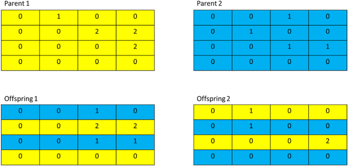
After parental pairs are selected, crossover is used to create two offspring. Crossover is performed by creating a new adjacency matrix for the offspring networks. For the new adjacency matrix each row is filled in using a row from one of the parental networks randomly (Figure 2).

Figure 2.

Representation of the crossover operation used in the model used in this paper. Each table represents the adjacency matrix of regulatory networks within a population. Crossover is performed by selecting rows from either parent randomly in order to create the adjacency matrix of the offspring.

The selection and crossover processes are repeated until one hundred offspring are created to form the next generation. Each offspring then undergoes mutation, node duplication/deletion and has its mutation and duplication/deletion rate modified as described below.

For each offspring, each index in the adjacency matrix has a chance of being mutated with a probability equal to the mutation rate it has inherited. This mutation sets the value of the index to either 0, or a positive or negative value of a functional group. This allows for each edge to be deleted, added, or functionally modified in the same mutation step.

2.1.5. Node duplication/deletion

After offspring networks were created using crossover and mutation, they undergo duplication/deletion which allows for networks to modify their size. Each individual has a duplication/deletion rate associated with it, which represented the probability that a node may be duplicated or deleted during the mutation step of the genetic algorithm. For each node a random number is generated, if it is equal to or less than the duplication/deletion rate, the node is selected for a “duplication/deletion” event. There is a 50%probability that the selected node is duplicated, which creates a new node that is added to the network, with all incoming and outcoming edges of the node being identical to the duplicated node. Figure 1 shows a network before and after a duplication event. Duplicated nodes are capable of gaining novel functions by mutation, such as the mutation shown in Figure 1 where a change from a positive to negative value changes an input into a “NOT” gate signified by a red edge between the nodes. If the selected node was not duplicated, then it is deleted by removing the node and all associated incoming and outgoing edges.

2.1.6. Mutation and duplication/deletion rate modification

Although the fitness (and therefore chance an individual is selected as a parent) is not dependent on the mutation rate or duplication/deletion rate these rates are inheritable and therefore successful individuals will pass on their rates with greater frequency. If a higher or lower mutation rate is beneficial (for example if higher mutation rates introduce deleterious mutations) then there should be some secondary selection for or against mutation and duplication/deletion rates. These rates are bounded between 0 and 1, as there cannot be less than a 0% or greater than a 100% chance of a mutation or duplication/deletion event occurring.

Each individual's rate of mutation and duplication/deletion is adjusted by the following formula, where RAN is a random number from 90 to 110 and Rate_g represents the mutation or duplication/deletion rate for the current generation:

$$Rat{e}_{g+1}=Rat{e}_g\ast \left(\frac{100}{RAN}\right)$$

This multiplicative random walk was used to represent the genetic basis of gene fidelity during reproduction: if an individual has a lower mutation rate there is a lower likelihood the DNA replication machinery mutates. Because of the bounds and the multiplication used, this produces a random walk which averages close to 0.5. This was used in favor of a more standard additive random walk, because a multiplicative random walk avoids large percentage updates in the mutation rate.

2.1.7. Identification and structural analysis of core networks

Core networks are determined from the final population as a post hoc analysis after the genetic algorithm run is complete. This is done to identify the nodes within a network which contribute to the period of the output signal, as some nodes may be effectively functionless. This is considered the core network because it is both necessary and sufficient to describe the behavior of the output of the network and used for later analysis. A series of attacks on each network was used to identify the critical components of the network.

Two different stuck-at-fault attacks are then applied to each non-input/output node in the network. An attack is performed by setting a node within a network to a value of either 1 or 0, creating 2 possible attacks per node. The stuck-at-fault value overrides the existing logic of the node. Our regular assessment of the network was performed: each potential input was given to the input node, and the resulting output from the output node was measured. If the resulting output does not equal O_i, the attack is then considered lethal, regardless of how close the output may be. If either attack is considered lethal then the attacked node is considered part of the core network.

2.1.8. A measure of population structural homogeneity

To assess how homogenous a population of networks is, we developed a measure of Evolutionary Edit Distance (EED). This is the minimum number of “evolutionary moves” which are required to transition from one network to another. This is derived from the “graph edit distance” which describes the number of moves necessary to transition from one graph to another. An evolutionary move is an addition, deletion, or modification of an edge between two nodes or the duplication/deletion of a node.

This distance score was based on the concept of “edit distance” from graph theory [36]. We can define the “Evolutionary distance” between two graphs G and G’’ similarly to how the graph edit distance can be defined [37]:

$$EED\left(G,G^{\prime }\right)=\underset{\forall (e1,e2\dots ek)\in E(G,G^{\prime })}{\min }\left\{\underset{(e1,e2\dots ek)}{CED\left(G,G^{\prime }\right)}\right\}$$

where CED represents the number of edits for each edit path e_i which would convert the graph G to G’. Because node duplication and node deletion may have different amounts of change in information, we cannot assume $EED\left(G,G^{\prime }\right)=EED(G^{\prime },G)$ when both graphs have different sizes. To accommodate for this, we measure the EED from the smaller network to the larger network only. The edit distance was then calculated by identifying the node-to-node bijection which had the smallest edit distance, where node substitutions could be performed by deleting one node and duplicating another. In the case of size differences, additional nodes were introduced by duplication rather than introducing null nodes. This allows us to determine how related two networks are together using only the moves allowed under our evolutionary algorithms. A standard graph edit distance may fall short in identifying similarities between networks because of the amount of information that can be added or removed from gene duplication and deletion events.

2.1.9. Rationale for fitness functions and alternative model

The fitness for the evolved networks is based on an oscillatory response to a given input signal. This was selected because oscillatory systems are widely seen in biological systems, with circadian patterns responding to external signals in nearly every domain of life. In order to confirm the general concepts demonstrated in this paper a secondary model was selected for evolution. We evolved networks based on evolving electronic circuits similar to those described previously [29]. These networks were evolved to replicate a 4 input/1 output truth table. The logic of each node is fixed to implicate a NAND gate. This model was modified so that the mutation rate was an inheritable trait and mutable in the same way as the oscillatory model described in this paper, however the network size remained fixed as per the original paper

Circuits were represented by an adjacency matrix, with a fixed number of nodes that encode NAND gates. There were four input nodes and one output node. The electronic circuit was evaluated with every possible combination of inputs (i.e. where the input nodes were all [0,0,0,0], [0,0,0,1], [0,0,1,0] and so forth). The set of inputs and the corresponding value of the output nodes were compiled into a truth table, and the fitness of the network was equal to the number of values on the truth table which corresponded with those of the target Boolean function. Tournament selection and crossover were performed identically with how it was done during for the oscillatory regulatory model described above. Mutation was performed as well, however each node in this model is limited to two input edges. If a new input edge was formed, one of the previous incoming edges would be removed. The duplication/deletion step was not performed, as these networks used a fixed number of nodes. After this the mutation rate would be modified for the offspring, as described above, and the process would repeat until sufficient offspring were created for the next generation.

The modified genetic algorithm (mGA) is described below.

Start mGA

initialize P

g = 0

 while g ≤ g_max

 g = g+1

 evaluate fitness of individuals in P

 select parents from individuals in P

 crossover parents to form offspring

 mutate offspring

 mutate mutation rate rates

 end while

end mGA

2.2. Simulations and computations

In all simulations, a population of “naïve” networks are initialized and then allowed to evolve toward a certain target function. These individuals are characterized as naïve because there is initially no logic associated between any of the nodes of the network within the population: all nodes have no inputs or outputs. This removes any possibility of a network randomly being very close to the target function and quickly reaching maximum fitness within the first generation. We considered a genetic algorithm run to be converged if half or more of its individuals had achieved maximum fitness. Simulations and calculations were performed on the Amarel high performance computing cluster at Rutgers University.

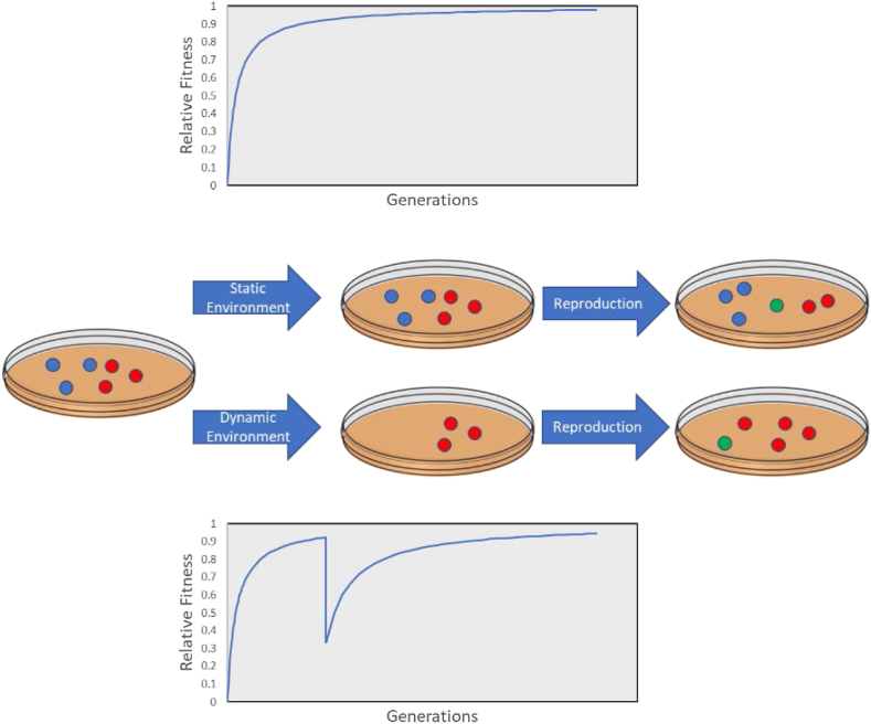
Two types of experiments were performed: those with a static fitness function and those with a dynamic target function with 2 epochs (Figure 3). These experiments were performed to compare populations in static environments to those in dynamic environments, and how their evolution may differ. For each condition, 500 genetic algorithm runs were performed, with each simulation producing a population. This was done to ensure at least 100 converged populations within the time limit, regardless of how complex the target function was. This provided a sufficient number of populations that achieved the proper target to study how networks evolve, especially in non-trivial conditions.

Figure 3.

The type of evolutionary experiments performed in this paper. The top represent the static experiments, where the fitness will increase and remain relatively static. The bottom shows the dynamic experiments where there is a shift in the target function, drastically reducing the fitness until the population can re-adapt.

2.2.1. Static target populations

A set of control simulations were performed in which the populations evolved toward a single target function. These control experiments allowed us to understand the basic behavior of the model, as well as confirm that the secondary selection of the mutation rate was occurring within our simulations. These simulations were run for different lengths of times to understand how long it may take a population to converge to a new function. For $\tau =3$ 50% of populations had converged by generation 1000, 62% at generation 3000, and 71% at generation 6000, and 89% by generation 10,000.

2.2.2. Dynamic target simulations

For the dynamic target experiments, the populations were evolved for a set amount of time with a target function of $\tau =3$ , however, during the final 2000 generations, the target function would be changed to $\tau =6$. Approximately 1/3 of simulations reached both the first and second target regardless of if the switch occurred at generation 1000 (29%), generation 3000 (34%), or generation 6000 (30%). The highest fitness individuals of converged populations would be used for calculating the evolutionary distance within and between populations, while individuals that were maladapted within the population would not be considered for structural analysis.

To compare evolving populations to fair controls, at the generation at which the second epoch began the population was replicated. One replication continued with the first target fitness, while the second replication continued into the second epoch. This would allow for a direct comparison between the same population und both static and dynamic environmental conditions.

The modified genetic algorithm, which evolved electronic circuit networks, were done using dynamic target simulations. One Boolean equation would be selected for the first epoch a second Boolean equation was used in the second epoch. The Boolean equations chosen were randomized for each simulation. These simulations were used to confirm that the secondary selection of mutation rate was not dependent on the network structure or function in the oscillatory regulatory functions used in this paper.

3. Results

3.1. Single target populations

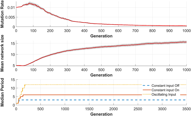
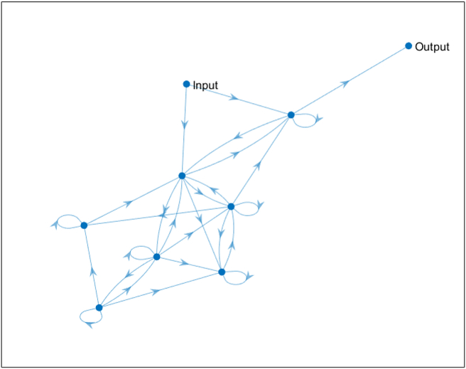
The naïve networks show a small increase in mutation rate and a rapid increase in network size, on average. The initial mutation rate was set to 0.01, and for τ = 3, the mutation rate had dropped to $4.97e^{-4}$ by generation 1000, a decrease of 95%, while the average network size increased from 5 nodes to 15 nodes (Figure 4 top and middle). A population's performance at a given generation is measured by comparing the oscillatory period of the output node O for each of the 3 different input signals previously described (Figure 4 bottom). The evolved networks tend to have be dense, with a number of parallel and nested feedback and feedforward loops. An example core network from a final population, for τ = 3 in a static environment can be seen in Figure 5, and the full networks often share similar densities and feedback loops.

Figure 4.

Top: The median mutation rate over time. The initial mutation rate starts as a fixed value and then allowed to adapt over time. Initially, the population selected for a higher mutation rate, followed by depression the mutation rate much lower than the initial rate. Middle: The median network size over time. Initially, there is a high network growth, with most of the network growth being done within the first 500–1000 generations. After this, the median size grows at a slower rate. Both of these graphs show the phasic nature of these traits: early in the evolutionary history of the population, there is a rapid change in mutation rate and size. As the populations converge to a single function, changes in these traits slow. Bottom: The median period for each of the three inputs. This population has a target of [3 6 12] for inputs of a constant 0 (off), constant 1 (on), an oscillating signal. Here we can see that the mean value of the outputs approaches the target function within the first several hundred generations.

Figure 5.

An example core network from a final population, for τ = 3 in a static environment. The core network includes seven intermediate nodes, an input node, and an output node. The network is dense, and representative of the core networks found in the populations. The full networks contain an average of 15 nodes, usually of similar connectivity. The networks consist of parallel and nested feedback loops, allowing for the creation of different oscillatory output signals in response to different input signals.

The tendency of the network size and mutation rate (and hence the number of mutations per generation) to increase initially existed regardless of the period of the target function of the population (τ value), although larger values of τ tended to have larger final networks. This would be expected, as more complex oscillatory signals require more nodes within the Boolean network. Higher mutation rates at this point would also be expected as a naïve network cannot make deleterious mutations: there are no functional connections that may be disrupted by mutations.

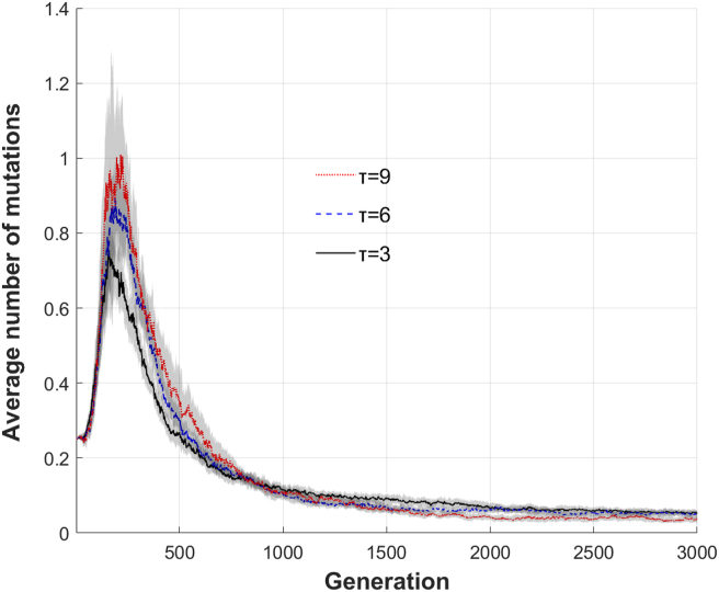
We hypothesize that the mutation rate decreased to a lower value in these more complex tasks because these larger networks are more vulnerable to being disrupted by changing the connections between components and further that the lower mutation rate is a response to the larger network size to decrease the number of mutations per generation. The mutation rate is partially dependent on the network size because each cell (potential edge) of the adjacency matrix has a chance to mutate therefore the larger the adjacency matrix, the greater chance a mutation will occur. Because of this the “per edge” mutation rate is converted into a “per generation” mutation rate, which is a function of the mutation rate and network size. In general, once the target function is found the number of mutations in each generation will approach 0, regardless of τ (Figure 6). Compared to the initial population, the average number of mutations per generation peaked at 404% (τ = 9), 357% (τ = 6), and 302%(τ = 3). By generation 1000 the number of mutations per generation is only 58% (τ = 9), 59%(τ = 6), and 54% (τ = 3). The percentages represent the number of mutations relative to the number of mutations at generation 1.

Figure 6.

The average number of mutations per generation, which is a function of the network size and the mutation rate, follows the same qualitative evolution regardless of function complexity. 95% confidence interval is shown in gray around the lines. The more complex the function, the more mutations occur at the maximum, but after the number of mutations peaks there will be a trend to minimize the number.

3.2. Changing environment simulations

The second set of simulations were used to measure how an evolved or evolving network would change in response to a new environmental stressor. These populations evolved with a target function of τ = 3 for 1000, 3000, and 6000 generations before changing the target function to τ = 6. The populations were given an additional 2000 generations to re-adapt to the new function to standardize the amount of time a population would have to re-adapt, regardless of its starting point. Similar to before, the fitness of individual networks was based entirely on the period of the output node, and not on a specific pattern.

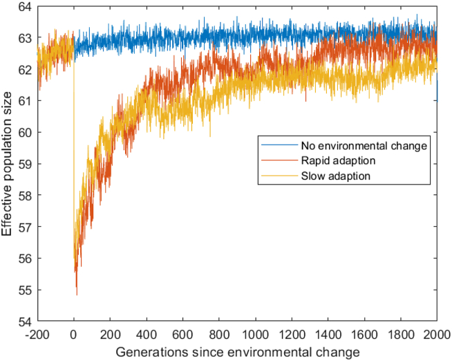
We compared the number of unique individuals who were selected each generation (the effective population size) and saw no significant difference between populations which adapted to the new function rapidly (in under 500 generations) and slowly (over 500 generations) (Figure 7).

Figure 7.

The number of individuals selected for reproduction for the next generation, which is the effective population size of the model. If all fitness was equal this would be approximately 63 individuals per generation on average. When an environmental shift occurs a smaller number of individuals are selected because the fitness gradient causes some individuals to be selected multiple times while others are not selected. The effective population size here is driven only by random chance in the selection stage and the relative fitness of individuals.

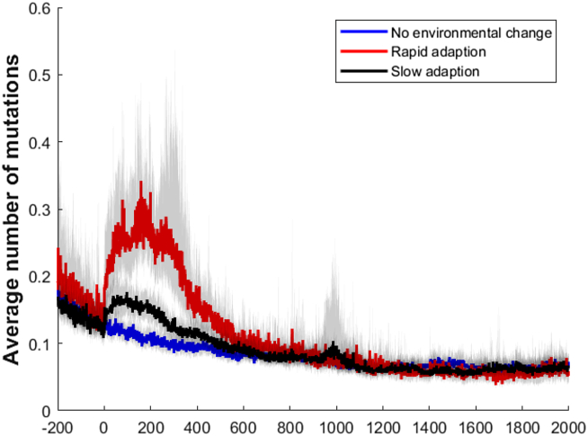
We compared three types of populations to understand how the mutation rate was affected by the environmental change: populations that retained the original target and had no new environmental stressor (a control), populations that quickly adapted to the new stressor (within 500 generations), and populations that adapted slower to the new stressor (over 500 generations). These populations were from separate simulations and had no interactions with one another. We found that populations that were rapid adapters would recover higher mutation rates shortly after the evolutionary target was changed, while populations that were slow to adapt would have a mild increase and those without any change in the evolutionary target would continue to decrease their mutation rate over time (Figure 8).

Figure 8.

The average number of mutations per generation for rapidly adapting, slow adapting, and non-adapting populations. Generation 0 represents the generation in which the change in fitness function was performed. Rapid mutating populations see a significantly higher number of mutations per generation initially after the switch in fitness function. Slowly adapting populations see an increase initially, as well, but it is much more modest. All the populations eventually reach similar number of generational mutations as they adapt to the new target.

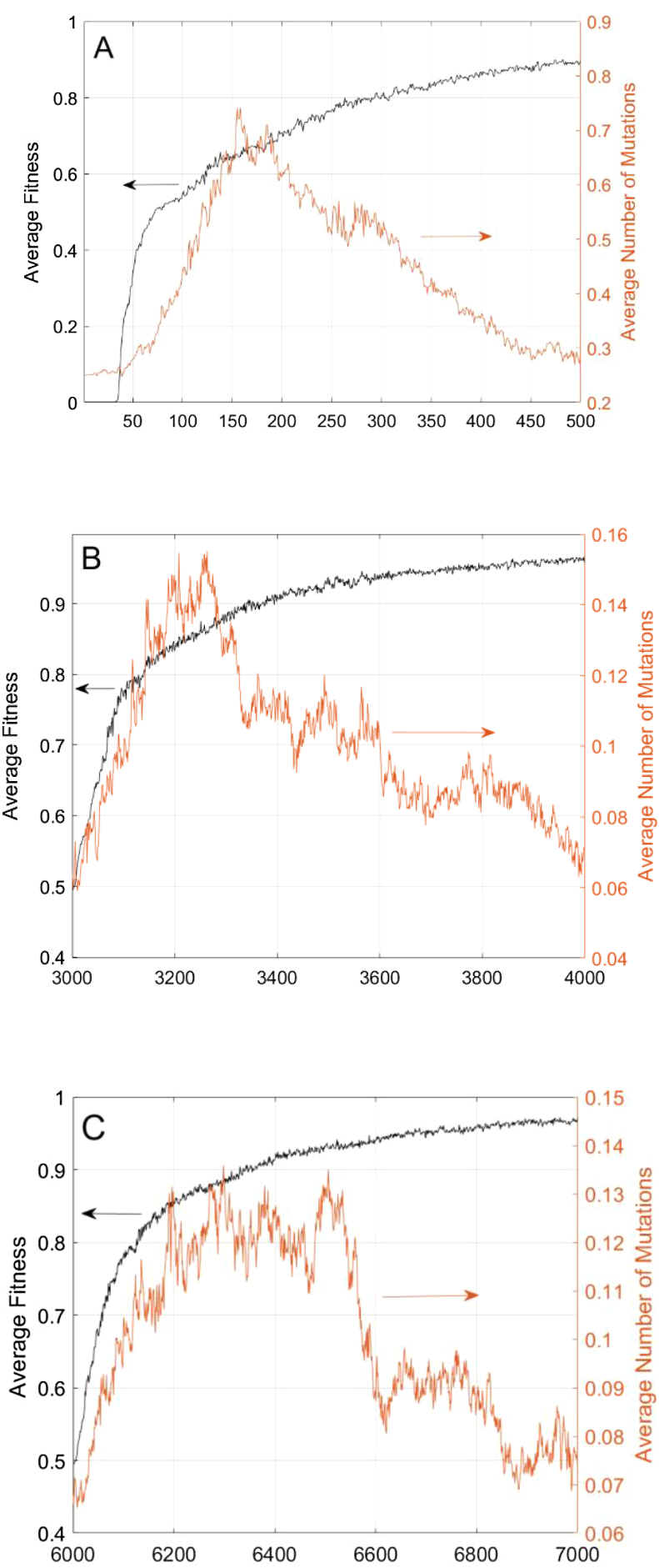
We see evidence of the mutation rate being selected for through secondary selection, due to the increase of the mutation rate after fitness increases, rather than the two increasing simultaneously. Figure 9 top shows the evolution of a naïve network, and the fitness sharply increased preceding an increase in the mutation rate. Figure 9 middle and bottom show the functional switch and generation 3000 and 6000, and the fitness recovers sharply at the same time as the change in the number of mutations. The populations do not start to suppress the number of mutations until after the fitness has begun to approach an asymptote, indicating that the population has reached a relatively stable state.

Figure 9.

The average population fitness compared to the average number of mutations during naïve evolution (A) and during evolution between two targets at generation 3000 (B) and 6000 (C) in all cases, the slope of the fitness function is steeper initially than the slope of the number of mutations, and the number of mutations does not decrease until after the average fitness has begun to reach an asymptote.

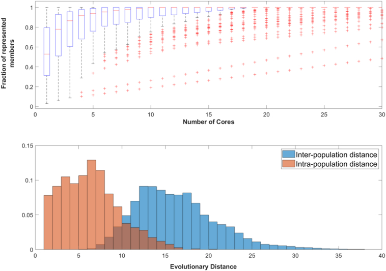
Sensitivity analysis of the networks allowed us to identify the core networks, which are the subnetworks necessary and sufficient to create the output of the network. These are considered “core” as the rest of the network had no impact on the output of the network even when they were disrupted. We used this to study the diversity of networks within populations, as many different networks may achieve the same signal transduction. Figure 10 top shows the number of unique cores in a population with a target function of τ = 3 at generation 1000. In this case, half of all populations have 90% or more of their individuals represented by 4 or fewer core networks, and half of all populations have 10 or fewer unique core networks within the population.

Figure 10.

Top: The distribution of the fraction of individuals whose function is characterized by a certain number of cores for τ = 3 at generation 1000. For each box plot, the fraction of individuals within a population who have that number of the most common cores are plotted. At 1 on the x-axis, the number of individuals within a population who share the most common core are plotted, at 5 the fraction of individuals who have the 5 most common cores are plotted. Over half of all populations have 90% or more of their networks represented by only 4 cores. While having a small number of cores is not a unique strategy, it is far more common than having a unique structure for each individual. Bottom: A histogram showing the distribution of evolutionary distances between individuals within the same population (red) and individuals from other populations (blue). We can see here that networks within the same populations are generally highly related, generally requiring 5 or fewer evolutionary moves to convert between the two individuals. In contrast, individuals from different populations have more differences. This implies that while there is a purifying selection within a population for highly related structures, different populations have not converged toward the same structure. The distributions were compared using a Kolmogorov–Smirnov test and determined to be different with a p-value < 0.01.

Once the core networks are identified, we used the EED to calculate how similar the core networks were within a population (the intra-population distance). This was compared to the evolutionary distance between of core networks between different populations (the inter-population distance). We found that populations were more consistent with themselves than they were with other populations with the same target τ (Figure 10 bottom). Populations should tend to have related networks because cross over and recombination will intermix networks within the population. We assume that populations will become homogenous over time because recombination between different networks is less likely to produce the same network output, while recombination between two identical networks should produce the same network and same phenotype.

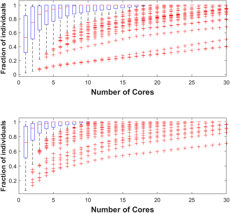
Populations from both types of simulations (those with a static target, and those with a dynamic target) were compared for their diversity. Over time the number of core functions that exist within a population decreased if there was only a single target. Populations that changed target functions maintained their population diversity of network structure, with an average of 53% of all networks sharing the same functional structure (Figure 11 top). However, if the target function remains the same, the number of unique structures drastically decreases, with an average of 67% of all networks sharing the same core structure (Figure 11 bottom).

Figure 11.

The diversity of network structures within a population with (top) an environmental shift and without (bottom) an environmental shift. This shows that the average number of unique, functional network structures within a population decreases while an environment remains static, but that the diversity of network structures may remain higher with a changing environment.

3.3. Electronic network evolution

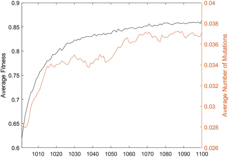
In order to confirm that any type of secondary selection of mutation rate originate from evolution, and not from the evolution of specific functions, the dynamic functions were repeated using evolution of electronic circuit networks. Each of these networks had 2 target Boolean functions which were selected randomly for the first and second target, as described before. We found a delay and secondary selection of mutation rate within these simulations as well (Figure 12). The fitness function of this model (Boolean equations formed from NAND gates) as well as general network structure (electronic circuits) were radically different from the oscillatory populations, but the apparent secondary selection of the mutation rate remains.

Figure 12.

The fitness and average number of mutations during the second epoch using the alternative electronic network model. Under this paradigm there is still a clear delay in the rise of the mutation rate.

4. Discussion

4.1. Single target populations

To understand how a population evolves in response to a changing environment, we need to compare it to a control condition: populations that are in truly static environments. Even in these conditions, the population does not remain static, with the network structures and mutation rates capable of evolving even after the population has achieved maximum fitness. Even as the phenotype of the population remains stable, the mutation rate will be depressed via secondary selection (Figure 4). The resulting networks often consist of nested and parallel feedback loops in order to produce the necessary oscillations, an example core network can be seen in Figure 5 showing the complexity of the networks capable of different oscillatory signals.

In our simulations all networks began as naïve networks: there were no logical connections between nodes that may influence the final structure of the network. All networks were given an initial evolutionary target. During this initial period, all populations appeared to have two general phases: one where the phenotype of the population exists on a gradient and the population is getting closer to the target function and another phase where the majority of the population has reached that target function. During the active phase, the fitness of individuals within the population are changing as the Boolean networks form into functioning systems. During the second phase, functional networks are present within the population however offspring may lose fitness due to deleterious mutations or recombinations between different networks present within the population.

This is important to understand because the average mutation rate across multiple populations should be determined in part by the probability of beneficial or deleterious mutations occurring within the offspring of the next generation. When the networks are initialized, the fitness of the entire population is at a minimum, and therefore no deleterious mutations may exist: all mutations will either be neutral or beneficial. In turn: as the population approaches maximum fitness, all mutations will be either neutral or deleterious. Within the context of these simulations, in addition to deleterious mutations, recombination of different network structures may result in a network with a different network output. This will limit the ability of every single offspring to maintain maximum fitness. We can see from these static environment experiments there will be secondary selection against both mutation rate as well as diversity. This serves primarily as a control for our changing environment simulations, as it is clear that there are no truly static evolutionary conditions in nature [38].

As would be expected the mutation rate appears to rise slightly on average during the first phase, when the population is starting to adapt to the target function, but not by a significant amount. Toward the end of this adaptation phase, the mutation rate goes down, asymptotically approaching 0. During this portion of the population's evolution, not every single individual will achieve maximum fitness. At this point, there is no new genetic variation which is necessary, although genetic variation can reduce the fitness of these individuals. Because of this, there is selection against high mutation rate individuals during this second phase, as those individuals will only have either neutral or deleterious mutations.

We performed these experiments with different target functions for populations, with increasing complexity and found that the expected mutation rate for each level of complexity was approximately the same. Regardless of the target period, every population had a decreasing mutation rate over time when there was a single target function. At generation 1000, the average number of mutations per generation was 58% (τ = 9), 59%(τ = 6), and 54% (τ = 3), Figure 6.

This decrease in mutation rate exists in populations that reach their target phenotype slowly: if an individual has a high fitness, but not maximum fitness, phenotype but does not have any beneficial mutations then deleterious mutations will still cause a loss of fitness. These deleterious mutations will cause maladapted populations to decrease their mutations rates to be protective of the fitness they did gain (Supplemental Figure 1). These maladapted populations had an average decrease of 70% from the start of the simulation through generation 1000, much greater than the decrease of any on-target population. This decreasing mutation rate is a protective mechanism that allows a population to maintain the fitness gains it has made, and so populations which have found second, or third best solutions would often see a decrease in mutation rate as well until a better solution was found. The maladapted populations have a larger decrease in the number of mutations compared to the populations which reach their target function within the time limit. This may indicate that the maladaptation is related to an overprotection of the population where higher mutation rates are overly selected against which slows the ability of the population to improve.

Fundamentally evolution is an inefficient process, and the interaction between adaptation and the mutation rate shows this. A depressed mutation rate may limit the ability of a population to adapt to a new environment, but a higher mutation rate may lead to an accumulation of deleterious mutations.

4.2. Changing environment simulations

To understand how populations, adapt under changing conditions we compare three population: Populations which rapidly adapted to the new target function, populations which slowly changed, and populations which did not have a change in environment. Here we see that populations with a change in environment underwent subpopulations selection very soon after the environment changes. This is represented by a decrease in the number of unique individuals selected to create offspring for the next generation (Figure 7). This may be thought of as a change in the effective population size of the populations, which may increase the drift within the populations shortly after the change in target. The effective population size of both rapid and slow adapting populations are similar, but the number of mutations in both groups is very different. This indicates that drift alone does not explain the mutation rate recovery in the rapidly adapting populations.

Interestingly, the number of mutations within each population before the environmental shift does not affect whether or not the population rapidly adapts (Supplemental Figure 2). Populations that have hypermutators or which have higher average mutation rates do not appear more likely to become rapidly adapting populations. The only common trait in rapidly adapting populations is the recovery of the mutation rate, not the initial mutation rate (Figure 8). Our populations see hitchhiking of high mutation rates with environmentally relevant mutation rates, and it appears that when higher mutation rates hitchhike with these traits there is faster adaptation. Secondary selection and hitchhiking, in this case, is entirely reliant on high mutation rate individuals consistently outperforming their low-mutation rate contemporaries. The hitchhiking effect is likely enhanced by the polygenic nature of our networks. Certain mutations will only be beneficial for certain network structures and not others, and therefore beneficial mutations from high mutation rate subpopulations may only be beneficial in the offspring of two individuals from the same sub-population. This further improves the relative fitness of the high mutation rate subpopulation, while limiting the ability of the mutator gene to be purged via recombination with the low mutation rate subpopulation. This effect seems to be independent as to when the environmental shift occurs there is always a delay in the evolution of mutation rate, a secondary selection of the high mutator population (Figure 9). We saw similar results for the delay in the evolution of mutation rate in the evolution of electronic circuit networks as well (Figure 12) and given the ubiquitous nature of oscillatory networks in biological systems we believe these results are not model or fitness specific.

The adaptive pressure, regardless of the speed of adaption, also drives diversity. Unlike static environments, where diversity decreases, diversity is maintained after the environmental shift. This is due to a combination of factors including a higher mutation rate as well as recent phenotypic diversity due to the fitness gradient within each population. Similar to the mutation rate, crossover and recombination may bring together beneficial genes that increase fitness or bring together incompatible mutations. In this sense, while there is active adaption toward a new phenotype, crossovers will increase network diversity and increase fitness. Once a population has converged, however, a crossover between distinct networks can only be neutral or deleterious and therefore diversity will be selected against.

The cause of the inter- and intra-population differences lies with adaptive processes and non-adaptive processes. Each population adapts a small number of strategies that fulfill the target function, and the selection of these strategies varies from population to population. For τ = 3 at generations 1000 there was an average of 53% of networks sharing the same core structure, and 50% of populations having 10 or fewer unique core structures (Figure 10 top). These structures appear to be divergent between populations. Within a single population, each core network has a median EED of 6, while between populations there is a median evolutionary distance of 15 (Figure 10 bottom). This divergence is strengthened over time as purifying selection and decreasing mutation rates limits the ability of conserved components to easily shift from one strategy to another. We can utilize the switched evolution simulations to see how time affects the diversity of structure. Comparing the structure of the networks before switching at generation 1000 to the structures of networks before switching at generation 3000 allows us to see this purifying selection in action. Over the course of 2000 generations, the percentage of the population which shared the identical functional network rose from 53% to 67% for τ = 3. The median number of unique core networks within an average population also decreased from 10 to 5, representing a nearly 50% decrease in the diversity of the populations. This highlights the importance of environmental stressors and competition in maintaining the diversity of a population. For the populations whose target switched from τ = 3 to τ = 6, there was no significant change in the fraction of networks with a single core network (53%), and 50% of networks had a median of 9 unique structures or fewer (Figure 11).

Rapidly changing environments are common: whether bacteria adapting to novel antibiotics or animals and plants adapting to changing environments due to climate change. The mechanisms and behaviors which drive adaption to changing environments may help understand why certain species thriving due to environmental changes, but many others go extinct as changing conditions become unsuitable for their survival [39, 40, 41, 42, 43]. We hope to expand this work to better understand not only how species adapt to stressors, but how multiple species and populations may interact and adapt to one another under stressful conditions.

Changes in the non-adaptive processes are seen as critical to overcoming stressors [2, 27, 28]. The flexibility of these non-random processes are also seen as important: bacteria with high mutation rates do not have better rates of survival in response to environmental stressors, but when wild type bacteria are exposed to environmental stressors their mutation rates will rapidly increase [2, 3, 4, 28].

5. Conclusions

Evidence of evolutionary advantage of mutation rates is often mixed: under certain circumstances, populations achieve higher mutation rates, or mutator populations attain higher fitness, although in other circumstances it is found that high mutation rates limit growth [2, 5, 14, 34, 42, 44, 45]. Our model shows that while a population is undergoing a “hill-climbing” behavior, with the fitness of the population increasing, there may be less selective pressure limiting the mutation rate.

Our model shows that even a sexually reproducing population may select for higher mutation rates while a population is moving along a fitness gradient, especially when undergoing rapid phenotypic adaption. This may be driven in part by the selection for functional networks, where networks with different features within the same population may undergo recombination and lose fitness similar networks undergoing recombination are more likely to retain the fitness gains of any de novo mutation. This does not directly contradict Lynch's drift barrier hypothesis: under conditions where novel mutations or novel phenotypes are beneficial the selection pressure against mutation rates will likely decrease as there are more theoretical beneficial mutations.

Our model has a limited number of mechanisms in terms of mutations, selection, and recombination. Despite this, we see both rapidly adapting populations as well as slowly adapting populations. In a theoretical case where an environmental shift may lead to extinction, we would only see a select few populations: a survivorship bias of those population which survived the extinction. We also hypothesize that there should be some survivorship bias in real-world populations: If we were to introduce an antibiotic to an agar plate then we could imagine a hypothetical population of bacteria that do not have any beneficial mutations. In this case, we would expect the mutation rate to remain primarily controlled by the effective population size, but the population would likely die off.

In contrast, if a beneficial mutation is found we expect the subpopulation which has created it to thrive. In the case of bacteria, this is often a hypermutator subpopulation [5, 46]. Although it may be easy to dismiss this as due to random genetic drift as the effective population size decreases it is difficult to ignore the fact that populations without hyper mutators will often fail to thrive even though their population size decreases. This means that even though increased mutation rates may be predicted only as a statistical anomaly under the neutral theory, it may become a statistical certainty when looking at a certain subset of populations (such as rapid phenotypic adaptions and evolutionary rescue), not due to a novel mechanism but rather due to chance and a survivorship bias. Due to this survivorship bias, it may be easy to mistake a statistical anomaly as a novel mechanism of adaption. Although, this may only be one factor in the rescue of a population which is stressed: in real-world populations other factors such as migration and gene-flow will play a role.

Declarations

Author contribution statement

Ioannis P. Androulakis:Conceived and designed the experiments; Analyzed and interpreted the data; Wrote the paper.

Matthew Putnins: Performed the experiments; Analyzed and interpreted the data; Contributed reagents, materials, analysis tools or data; Wrote the paper.

Funding statement

This work was supported by National Institutes of Health (GM131800).

Data availability statement

No data was used for the research described in the article.

Declaration of interests statement

The authors declare no conflict of interest.

Additional information

No additional information is available for this paper.

Appendix A. Supplementary data

The following is the supplementary data related to this article:

References

- 1.Svensson E.I., Berger D. The role of mutation bias in adaptive evolution. Trends Ecol. Evol. 2019;34:422–434. doi: 10.1016/j.tree.2019.01.015. [DOI] [PubMed] [Google Scholar]
- 2.Komp Lindgren P., Karlsson A., Hughes D. Mutation rate and evolution of fluoroquinolone resistance in Escherichia coli isolates from patients with urinary tract infections. Antimicrob. Agents Chemother. 2003;47:3222–3232. doi: 10.1128/AAC.47.10.3222-3232.2003. [DOI] [PMC free article] [PubMed] [Google Scholar]
- 3.Lynch M. The evolution of genetic networks by non-adaptive processes. Nat. Rev. Genet. 2007;8:803–813. doi: 10.1038/nrg2192. [DOI] [PubMed] [Google Scholar]
- 4.Lynch M. Evolution of the mutation rate. Trends Genet. 2010;26:345–352. doi: 10.1016/j.tig.2010.05.003. [DOI] [PMC free article] [PubMed] [Google Scholar]
- 5.Swings T. Adaptive tuning of mutation rates allows fast response to lethal stress in Escherichia coli. Elife. 2017;6 doi: 10.7554/eLife.22939. [DOI] [PMC free article] [PubMed] [Google Scholar]
- 6.Knabe J.F., Nehaniv C.L., Schilstra M.J. Do motifs reflect evolved function?--No convergent evolution of genetic regulatory network subgraph topologies. Biosystems. 2008;94:68–74. doi: 10.1016/j.biosystems.2008.05.012. [DOI] [PubMed] [Google Scholar]
- 7.Ingram P.J., Stumpf M.P., Stark J. Network motifs: structure does not determine function. BMC Genom. 2006;7:108. doi: 10.1186/1471-2164-7-108. [DOI] [PMC free article] [PubMed] [Google Scholar]
- 8.Parter M., Kashtan N., Alon U. Facilitated variation: how evolution learns from past environments to generalize to new environments. PLoS Comput. Biol. 2008;4 doi: 10.1371/journal.pcbi.1000206. [DOI] [PMC free article] [PubMed] [Google Scholar]
- 9.Stelling J., Klamt S., Bettenbrock K., Schuster S., Gilles E.D. Metabolic network structure determines key aspects of functionality and regulation. Nature. 2002;420:190–193. doi: 10.1038/nature01166. [DOI] [PubMed] [Google Scholar]
- 10.Bhan A., Galas D.J., Dewey T.G. A duplication growth model of gene expression networks. Bioinformatics. 2002;18:1486–1493. doi: 10.1093/bioinformatics/18.11.1486. [DOI] [PubMed] [Google Scholar]
- 11.Jensen J.D. The importance of the neutral theory in 1968 and 50 years on: a response to Kern and Hahn 2018. Evolution. 2019;73:111–114. doi: 10.1111/evo.13650. [DOI] [PMC free article] [PubMed] [Google Scholar]
- 12.Kern A.D., Hahn M.W. The neutral theory in light of natural selection. Mol. Biol. Evol. 2018;35:1366–1371. doi: 10.1093/molbev/msy092. [DOI] [PMC free article] [PubMed] [Google Scholar]
- 13.Sung W., Ackerman M.S., Miller S.F., Doak T.G., Lynch M. Drift-barrier hypothesis and mutation-rate evolution. Proc. Natl. Acad. Sci. Unit. States Am. 2012;109:18488–18492. doi: 10.1073/pnas.1216223109. [DOI] [PMC free article] [PubMed] [Google Scholar]
- 14.Sprouffske K., Aguilar-Rodriguez J., Sniegowski P., Wagner A. High mutation rates limit evolutionary adaptation in Escherichia coli. PLoS Genet. 2018;14 doi: 10.1371/journal.pgen.1007324. [DOI] [PMC free article] [PubMed] [Google Scholar]
- 15.Heilbron K., Toll-Riera M., Kojadinovic M., MacLean R.C. Fitness is strongly influenced by rare mutations of large effect in a microbial mutation accumulation experiment. Genetics. 2014;197:981–990. doi: 10.1534/genetics.114.163147. [DOI] [PMC free article] [PubMed] [Google Scholar]
- 16.Ohta T. Near-neutrality in evolution of genes and gene regulation. Proc. Natl. Acad. Sci. Unit. States Am. 2002;99:16134–16137. doi: 10.1073/pnas.252626899. [DOI] [PMC free article] [PubMed] [Google Scholar]
- 17.Lynch M. Evolutionary layering and the limits to cellular perfection. Proc. Natl. Acad. Sci. Unit. States Am. 2012;109:18851–18856. doi: 10.1073/pnas.1216130109. [DOI] [PMC free article] [PubMed] [Google Scholar]
- 18.van Noort V., Snel B., Huynen M.A. The yeast coexpression network has a small-world, scale-free architecture and can be explained by a simple model. EMBO Rep. 2004;5:280–284. doi: 10.1038/sj.embor.7400090. [DOI] [PMC free article] [PubMed] [Google Scholar]
- 19.Meshi O., Shlomi T., Ruppin E. Evolutionary conservation and over-representation of functionally enriched network patterns in the yeast regulatory network. BMC Syst. Biol. 2007;1 doi: 10.1186/1752-0509-1-1. 1-1, [DOI] [PMC free article] [PubMed] [Google Scholar]
- 20.Siepel A. Evolutionarily conserved elements in vertebrate, insect, worm, and yeast genomes. Genome Res. 2005;15:1034–1050. doi: 10.1101/gr.3715005. [DOI] [PMC free article] [PubMed] [Google Scholar]
- 21.Wuchty S., Oltvai Z.N., Barabasi A.L. Evolutionary conservation of motif constituents in the yeast protein interaction network. Nat. Genet. 2003;35:176–179. doi: 10.1038/ng1242. [DOI] [PubMed] [Google Scholar]
- 22.Chung F., Lu L., Dewey T.G., Galas D.J. Duplication models for biological networks. J. Comput. Biol. 2003;10:677–687. doi: 10.1089/106652703322539024. [DOI] [PubMed] [Google Scholar]
- 23.Eisenberg E., Levanon E.Y. Preferential attachment in the protein network evolution. Phys. Rev. Lett. 2003;91:138701. doi: 10.1103/PhysRevLett.91.138701. [DOI] [PubMed] [Google Scholar]
- 24.Stumpf M.P., Wiuf C., May R.M. Subnets of scale-free networks are not scale-free: sampling properties of networks. Proc. Natl. Acad. Sci. Unit. States Am. 2005;102:4221–4224. doi: 10.1073/pnas.0501179102. [DOI] [PMC free article] [PubMed] [Google Scholar]
- 25.Han J.-D.J. Evidence for dynamically organized modularity in the yeast protein–protein interaction network. Nature. 2004;430:88–93. doi: 10.1038/nature02555. [DOI] [PubMed] [Google Scholar]
- 26.Arita M. The metabolic world of Escherichia coli is not small. Proc. Natl. Acad. Sci. Unit. States Am. 2004;101:1543–1547. doi: 10.1073/pnas.0306458101. [DOI] [PMC free article] [PubMed] [Google Scholar]
- 27.Lavergne S., Muenke N.J., Molofsky J. Genome size reduction can trigger rapid phenotypic evolution in invasive plants. Ann. Bot. 2010;105:109–116. doi: 10.1093/aob/mcp271. [DOI] [PMC free article] [PubMed] [Google Scholar]
- 28.Swings T. Adaptive tuning of mutation rates allows fast response to lethal stress in Escherichia coli. Elife. 2017;6 doi: 10.7554/eLife.22939. [DOI] [PMC free article] [PubMed] [Google Scholar]
- 29.Kashtan N., Alon U. Spontaneous evolution of modularity and network motifs. Proc. Natl. Acad. Sci. U. S. A. 2005;102:13773–13778. doi: 10.1073/pnas.0503610102. [DOI] [PMC free article] [PubMed] [Google Scholar]
- 30.Burda Z., Krzywicki A., Martin O.C., Zagorski M. Motifs emerge from function in model gene regulatory networks. Proc. Natl. Acad. Sci. U. S. A. 2011;108:17263–17268. doi: 10.1073/pnas.1109435108. [DOI] [PMC free article] [PubMed] [Google Scholar]
- 31.Alon U. Network motifs: theory and experimental approaches. Nat. Rev. Genet. 2007;8:450–461. doi: 10.1038/nrg2102. [DOI] [PubMed] [Google Scholar]
- 32.Wilke C.O., Wang J.L., Ofria C., Lenski R.E., Adami C. Evolution of digital organisms at high mutation rates leads to survival of the flattest. Nature. 2001;412:331–333. doi: 10.1038/35085569. [DOI] [PubMed] [Google Scholar]
- 33.Johnson T.J.G. Beneficial mutations, hitchhiking and the evolution of mutation rates in sexual populations. Genetics. 1999;151:1621–1631. doi: 10.1093/genetics/151.4.1621. [DOI] [PMC free article] [PubMed] [Google Scholar]
- 34.Theodorakis C.W., Lee K.-L., Adams S.M., Law C.B. Evidence of altered gene flow, mutation rate, and genetic diversity in redbreast sunfish from a pulp-mill-contaminated river. Environ. Sci. Technol. 2006;40:377–386. doi: 10.1021/es052095g. [DOI] [PubMed] [Google Scholar]
- 35.Androulakis I.P., Venkatasubramanian V. A genetic algorithmic framework for process design and optimization. Comput. Chem. Eng. 1991;15:217–228. [Google Scholar]
- 36.Gao X., Xiao B., Tao D., Li X. A survey of graph edit distance. Pattern Anal. Appl. 2009;13:113–129. [Google Scholar]
- 37.Serratosa F. Graph edit distance: restrictions to be a metric. Pattern Recogn. 2019;90:250–256. [Google Scholar]
- 38.Reznick D.N., Ghalambor C.K. Springer; 2001. Microevolution Rate, Pattern, Process 183-198. [Google Scholar]
- 39.Ceballos G. Accelerated modern human–induced species losses: entering the sixth mass extinction. Sci. Adv. 2015;1 doi: 10.1126/sciadv.1400253. [DOI] [PMC free article] [PubMed] [Google Scholar]
- 40.De Vos J.M., Joppa L.N., Gittleman J.L., Stephens P.R., Pimm S.L. Estimating the normal background rate of species extinction. Conserv. Biol. 2015;29:452–462. doi: 10.1111/cobi.12380. [DOI] [PubMed] [Google Scholar]
- 41.Bradshaw W., Holzapfel C. Genetic response to rapid climate change: it's seasonal timing that matters. Mol. Ecol. 2008;17:157–166. doi: 10.1111/j.1365-294X.2007.03509.x. [DOI] [PubMed] [Google Scholar]
- 42.Gienapp P., Teplitsky C., Alho J., Mills J., Merilä J. Climate change and evolution: disentangling environmental and genetic responses. Mol. Ecol. 2008;17:167–178. doi: 10.1111/j.1365-294X.2007.03413.x. [DOI] [PubMed] [Google Scholar]
- 43.Sirisena P., Noordeen F. Evolution of dengue in Sri Lanka—changes in the virus, vector, and climate. Int. J. Infect. Dis. 2014;19:6–12. doi: 10.1016/j.ijid.2013.10.012. [DOI] [PubMed] [Google Scholar]
- 44.Shaver A.C. Fitness evolution and the rise of mutator alleles in experimental Escherichia coli populations. Genetics. 2002;162:557–566. doi: 10.1093/genetics/162.2.557. [DOI] [PMC free article] [PubMed] [Google Scholar]
- 45.Bosshard L. Accumulation of deleterious mutations during bacterial range expansions. Genetics. 2017;207:669–684. doi: 10.1534/genetics.117.300144. [DOI] [PMC free article] [PubMed] [Google Scholar]
- 46.Maciá M.D. Hypermutation is a key factor in development of multiple-antimicrobial resistance in Pseudomonas aeruginosa strains causing chronic lung infections. Antimicrob. Agents Chemother. 2005;49:3382–3386. doi: 10.1128/AAC.49.8.3382-3386.2005. [DOI] [PMC free article] [PubMed] [Google Scholar]
Associated Data
This section collects any data citations, data availability statements, or supplementary materials included in this article.
Supplementary Materials