Abstract
COVID-19 made considerable changes in the lifestyle of people, which have led to a rise in energy use in homes. So, this study investigated the relationship between COVID-19 and domestic hot water demands. For this purpose, a nondimensional and principal component analysis were conducted to find out the influencing factors using demand data before and after COVID-19 from our study site. Analysis showed that the COVID-19 outbreak affected the daily peak time and the amount of domestic hot water usage, the active case number of COVID-19 was a good indicator for correlating the changes in hot water demand and patterns. Based on this, a machine learning model with an artificial neural network was developed to predict hot water demand depending on the severity of COVID-19 and the relevant correlation was also derived. The model analysis showed that the increase in the number of active cases in the region affected the hot water demand increased at a certain rate and the maximum demand peak in morning during weekdays and weekends decreased. Furthermore, if the number of active cases reached more than 4000, the peak in morning moved to afternoon so that the energy use patterns of weekdays and weekends are assimilated.
Keywords: COVID-19, Domestic hot water, Artificial neural network
Nomenclature
hourly domestic hot water usage
normalized hourly domestic hot water usage
- A
list of hourly domestic hot water usage for the day
- AC
number of active case (log10)
- A
normalized list of hourly domestic hot water usage for the day
- b
bias
- Cp
specific heat capacity (kJ kg−1 K−1)
- h
hour (h)
- m
mass flow rate (kg h−1)
- n
number of datapoints
- Q
domestic hot water demand (MWh)
- Qinc
increase of domestic hot water demand by the COVID-19 (%)
- R2.
coefficient of determination
- T
temperature (°C)
- w
weight
- X
input
- x
standardized input
- Y
output
averaged output
- y
standardized output
Greek letters
- μ
mean
- σ
standard deviation
Subscripts
- cw
city water
- i
index of households
- inc
increment
- j
neuron number in input layer
- k
neuron number in first hidden layer
- l
neuron number in second hidden layer
- m
neuron number in third hidden layer
- nw
nationwide
- pred
prediction
- sma
Seoul metropolitan area
Acronyms
- ANN
artificial neural network
- CHP
combined heat and power
- COV
covariance
- COVID-19
Severe Acute Respiratory Syndrome-Coronavirus-2 (SARS-CoV-2)
- DHW
domestic hot water
- HEX
heat exchanger
- KPCA
kernel principal component analysis
- MAE
mean absolute error
- MSLE
mean squared log error
- ND
non-dimensional
- PC
principal component
- PCA
principal component analysis
- ReLU
rectified linear unit
- RMSE
root mean square error
- SH
space heating
1. Introduction
The COVID-19 pandemic changed the overall industrial ecosystem and the daily life of people [[1], [2], [3], [4], [5]], and the energy industry was unable to avoid such changes either [6,7]. Changes in life patterns brought unexpected shock to the production and demand system of the energy industry; in particular, they brought considerable changes in areas such as energy consumption, energy demand peak, and demand [8,9]. The International Energy Agency (IEA) published a study result that global energy demand in the first quarter of 2020 was decreased by 3.8% from the previous year and predicted that the demand will decrease by 6% in 2020. Furthermore, it was reported that throughout the world, coal demand will decrease by 8%, petroleum demand by 5%, and aviation fuel by 25% in the first quarter of 2020 [10].
Changes in energy demand caused by COVID-19 are deeply related to local communities, national and global fossil energies, and new renewable energy supply and demand, thereby causing a large impact on these issues. Therefore, numerous studies were conducted to analyze the effects of COVID-19 on energy demand to relieve the shock [[11], [12], [13]].
Werth et al. [14] analyzed the effects of COVID-19 on the energy grid market in Europe. Because of COVID-19, electricity consumption in each European country was largely decreased, which caused a tremendous negative impact on the development of electric power generation. To provide solutions for this problem, methods such as energy trade between countries and the modification of new renewable energy production plans were proposed. Through a simulation on complex buildings, Zhang et al. [15] predicted that electricity consumption will increase by 14.3%–18.7%, whereas space heating (SH), space cooling, and domestic hot water (DHW) consumption will decrease by 7.1%–12.0% after COVID-19.
In addition to changes in energy use at national or governmental levels, certain studies were conducted to analyze the increase or decrease in energy consumption based on changes in life patterns at residential buildings, which accounts for 20% of the global energy consumption (2018) [16]. Most studies related to energy in industry and transportation fields predicted that energy demand will decrease. However, other studies, which suggested that the energy consumption of residential buildings will rather increase, were more common. Zanocco et al. [17] studied the effects of Shelter in Place Order of California on the life patterns of people, changes in domestic energy consumption, and the prospect of smart home technology. Cvetkovic et al. [18] analyzed changes in behavioral patterns of people in residential spaces because of COVID-19 and predicted that natural gas, electricity, and water consumption will largely increase. Cheshmehzangi [19] analyzed the impact of COVID-19 on transportation, food, leisure, air conditioning and heating, and lighting energy consumption in residential buildings and reported that changes in transportation, air conditioning, and heating energy were particularly significant.
An accurate understanding of energy consumption is important for establishing national, municipal, or building level energy policy, and for the effective utilization of energy sources. Because energy demand characteristics were largely changed by the effect of the COVID-19 pandemic, conducting studies for increasing the understanding of energy consumption in this situation is important. Although certain studies were conducted on changes in energy demand caused by COVID-19, most studies focused on the electricity sector. Among the various types of energy, heat energy accounts for approximately 69% of the total energy amount used in residential area, and approximately 23% of heat energy is used in hot water [16], which accounts for a large proportion in the total energy consumption. However, studies conducted on analyzing the importance of heat demand are relatively insufficient. This is because DHW sub-meters are not installed wherein individual heating systems. Although the DHW sub-meters separately measures the hot water demand wherein district heating systems, they normally measure only the accumulated flow, not the heat consumption. In the district heating system, measuring the calorific amount of SH is easy as the sub-metering uses a difference between the supply and return temperatures. However, it is difficult to measure the calorific value of DHW because the difference between hot water temperature in each household and make-up city water temperature in a central substation needs to be measured.
The purpose of this study is to identify changes in DHW demand and usage patterns caused by the COVID-19 pandemic, and a correlation between the transmission rate of the COVID-19 and DHW consumption, to develop a prediction model that clarifies the effects of COVID-19. A district heating supplied apartment complex with 16 buildings, 918 households was selected to collect demand data and develop the model. Thereafter, the actual DHW consumption amount and climate data gathered for three years in the complex were combined to analyze the following from various aspects such as hourly, daily, monthly, and on weekdays/weekends: changes in DHW demand before and after the outbreak of COVID-19, DHW demand pattern by hours, and cause-and-effect relationship with external factors. Major factors that affect DHW consumption characteristics were extracted, and their correlation was analyzed. Based on these results, machine learning model with an artificial neural network (ANN) that can predict the DHW consumption by climatic conditions, time, and COVID-19 conditions was developed. Through this model, the actual consumption amount based on the spread of COVID-19, and changes in the DHW consumption patterns were identified. Moreover, a mathematical correlation was proposed to predict the rate of increase in DHW consumption because of the transmission rate of COVID-19.
2. Description of measuring data
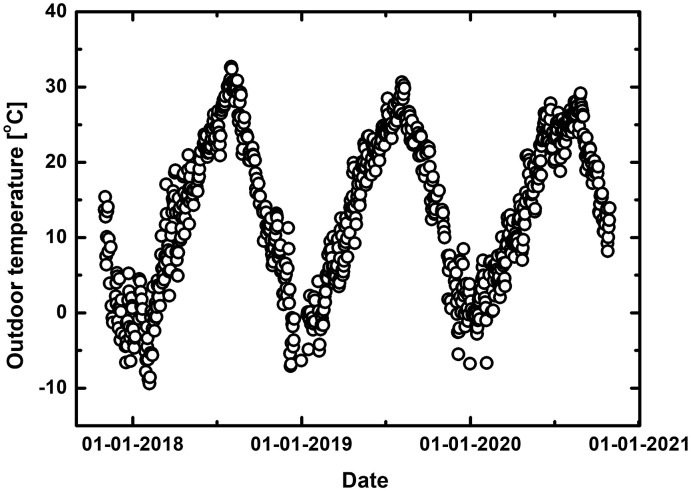
The place for data collection was an apartment complex in Seongnam-si, Gyeonggi-do, Republic of Korea, which belongs to one of the regions in the Seoul metropolitan area. This region has a representative continental climate characteristic and a large temperature difference throughout a year having four distinct seasons [20]. Fig. 1 shows the outdoor temperature in the region between November 2017 and October 2020, and Table 1 shows the information of the region and our study site.
Fig. 1.
Changes in the trend of outdoor temperature in the region during the past three years.
Table 1.
General information of country and study site.
| Information | Description | |
|---|---|---|
| Population (Nationwide) | 51.78 million (2019) [21] | |
| Population (Seoul metropolitan area) | 25.89 million (2019) [21] | |
| Climate of the country | 'Dwa' in Köppen-Geiger classification | |
| Our study site information | Location | Gyeonggi province, Republic of Korea (Located in Seoul metropolitan area) Latitude: 37.378, Longitude: 127.118 |
| Housing type | Apartment complex (16 buildings) | |
| Number of households | 918 | |
| Floor areas | 103–228 m2 | |
| Heat supply method | District heating Four pipe system having central substation Separate central SH and DHW heat exchanger |
|
| Sub-metering method | SH and DHW submeters in each household | |
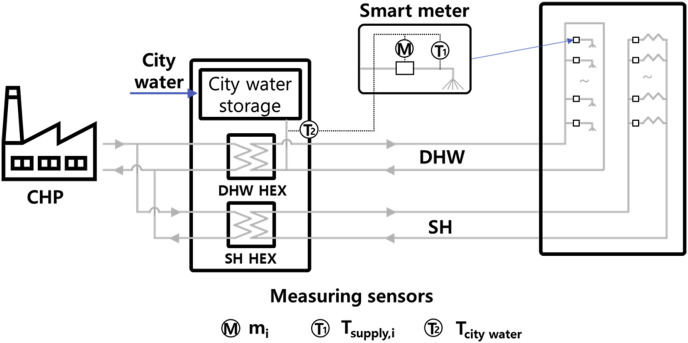
Fig. 2 shows the detailed secondary side with DHW submetering in the district heating system. After the heat is delivered from the CHP via the primary side to the central substation of the apartment, the exchanged heat is distributed as the SH and DHW to each household. The calorific amount of DHW used by each household can be measured by combining city water temperature measured in the central substation, hot water temperature and flow rate measured by DHW smart meter in each household [22]. The calorific amount of DHW for all the entire 918 households in the apartment complex can be calculated through Eq. (1):
| (1) |
Fig. 2.
The district heating system and the secondary side DHW sub-metering using smart meter.
The gathered information includes DHW accumulated energy, flow, temperatures, and household information. Table 2 shows the data type of this information. This study used hourly data, and data collection simultaneity was maintained within 15 s to minimize the time mismatch of energy usage. In this study, the analysis was conducted based on data gathered from November 2017 to October 2020.
Table 2.
Information on the gathered data.
| Information | Description |
|---|---|
| Period | From 11–01–2017 to 10-31-2020 |
| Data interval used | One hour |
| Data collection simultaneity | 15 s |
| Measuring parameter | DHW energy and flow usage, flow rate, supply temperature, city water temperature, outdoor temperature |
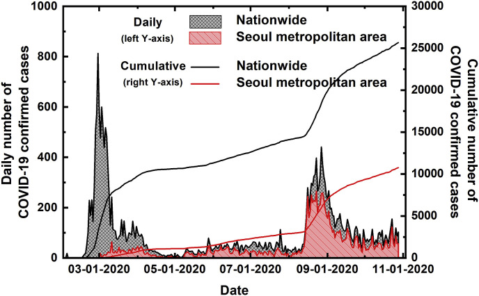
In Republic of Korea, after the first COVID-19 confirmed case emerged on January 20, 2020, the accumulative number of confirmed cases steadily increased to reach 26511 by October 31, 2020. During that time, two large waves of COVID-19 occurred where the first wave mostly occurred in regions located 270 km away from the study site; however, the second wave occurred at Seoul metropolitan area where the study site is located. Fig. 3 shows the daily number of COVID-19 confirmed cases and the accumulated number of confirmed cases throughout the nationwide and the Seoul metropolitan area. The first and second waves occurred in mid-February and mid-August 2020, respectively, and COVID-19 confirmed cases have steadily emerged since then.
Fig. 3.
Trend comparison of the daily number of COVID-19 confirmed cases.
3. Analysis of changes in DHW demand caused by COVID-19
3.1. Changes in DHW demand
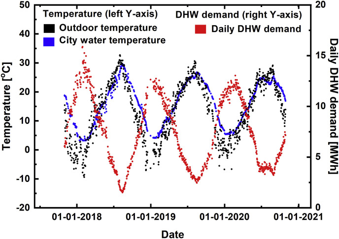
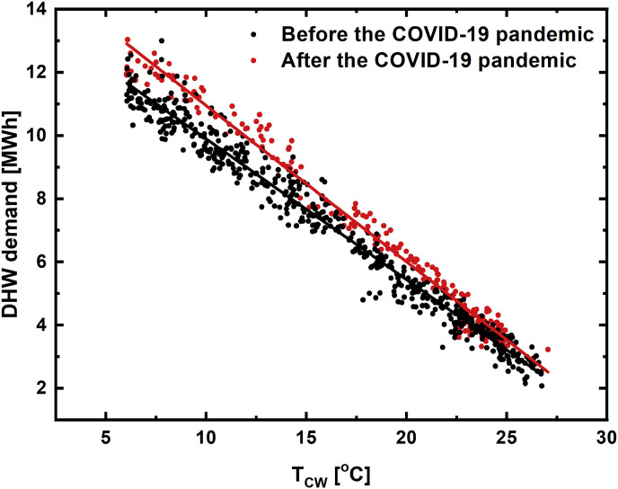
Fig. 4 compares changes in the daily outdoor temperature of the study site, daily average city water temperature, and daily average DHW demand. Trends showed that changes in city water temperature follow the changes in outdoor temperature after several days, and DHW demand shows the opposite trend from the city water temperature. Because DHW demand is highly related with the city water temperature, it decreases in summer when the city water temperature is high, as shown in Fig. 5 .
Fig. 4.
Trend comparison of the daily outdoor temperature, city water temperature, and DHW demand.
Fig. 5.
Changes in DHW demand based on the city water temperature before and after the COVID-19 pandemic.
Fig. 5 shows the relationship between DHW demand and the city water temperature before and after the COVID-19 pandemic, where black circular points show DHW demand before the COVID-19 pandemic (based on February 16, 2020), and red circular points show the same after the pandemic. Under the same city water temperature condition, DHW demand after the COVID-19 significantly increased compared to pre COVID-19. Therefore, it can be inferred that DHW demand largely increased during the COVID-19 pandemic because of changes in the life patterns of people such as the lockdown policy, working from home, closing of schools, and increased awareness of personal hygiene. In some period (around 15 and 23 °C of city water temperature), the increased DHW demand seems to be temporarily small. This is because the number of COVID-19 cases during the period (early May, early August) was small, and the life pattern was similar to that of pre-COVID-19 years as shown in Fig. 3, Fig. 4.
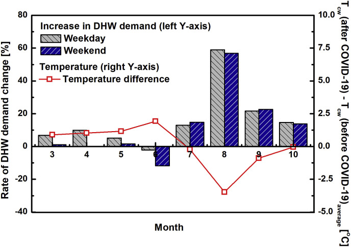
Fig. 6 shows the monthly rate of DHW demand change after the COVID-19 pandemic and difference in the city water temperature before (average of the past 3 years) and after COVID-19. If the city water temperatures difference before and after COVID-19 (red square and line) is more than 0, it indicates that the monthly city water temperature in 2020 was higher than the previous city water temperature. DHW demand after the outbreak of COVID-19 is higher and demand increased more during weekdays compared to weekends. This is presumed to be because in-house hours and the number of people staying inside during the weekdays are increased. The maximum increase in the DHW demand was observed in August, the second period when the number of confirmed cases rapidly increased, to reach up to 58.98%. However, these rates of increase cannot be assumed to be simply caused by COVID-19 because the city water temperature was coupled except for July and October 2020, when the average city water temperature was similar to the previous year. August 2020 was a month when the number of COVID-19 confirmed cases rapidly increased. However, the city water temperature in August 2021 was 3.48 °C lower than the annual average because of the record-breaking abnormal temperature. Thus, the increase in DHW demand was caused by a combination of the COVID-19 pandemic and low city water temperature. Moreover, although June 2020 showed the reduced DHW demand, the fact that city water temperature was rather higher compared to the previous year shall be considered. Therefore, there exists a limitation in decoupling the reason of the rate of DHW demand change caused only by COVID-19 when the DHW demand is simply compared with past data.
Fig. 6.
Increase rate of the monthly DHW demand after the COVID-19 pandemic and annual difference in the city water temperature.
3.2. Change in daily demand pattern
As daily DHW demand pattern has a tendency where most of the demands are located in peak hours, it requires a different approach method than the daily demand analysis method. In general, the daily DHW demand pattern shows two peak periods, i.e., one each in morning and afternoon [23], and this was also similar in this study. In addition, because of changes in life patterns caused by the COVID-19 pandemic, large changes occurred not only in the abovementioned daily and monthly DHW demand but also in the daily DHW demand pattern.
To analyze only the hourly demand pattern by excluding changes caused by climatic or seasonal changes, the daily DHW demand was normalized into values between 0 and 1 through min-max normalization, which is shown in Eq. (2) [24].
| (2) |
In this equation, A is the list of hourly demand on a day, which is expressed as , and the range of i is 0–23. refers to the specific demand between i hour and i + 1 h is the maximum hourly DHW demand in a day, is the minimum hourly DHW demand in a day. The normalized hourly demand is and the list of the can be expressed as . Also, is 0 and should be 1.
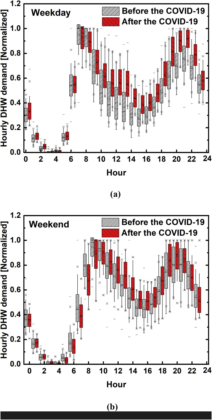
In general, the DHW demand pattern is largely affected by the presence of holidays [25,26]. Fig. 7 shows box plot comparison in demand pattern on weekdays and weekends before/after COVID-19 pandemic. For weekdays, the peak demand at 07:00–08:00 is similar before and after the COVID-19 pandemic, but the value has increased at every hour after the COVID-19 pandemic. This implies that the usage at peak demand has relatively decreased. It was determined that this phenomenon was caused because activities in workplaces and schools, which are the major causes of DHW demand peak in weekday's morning time, were replaced by causes such as working from home and self-learning. Moreover, it can be presumed that the DHW demand rate increased in afternoon and night because of the increased number of people staying inside. During weekends, although DHW demand peak time in morning was slightly lesser, changes in the pattern are not as large as that during weekdays.
Fig. 7.
Comparison of the hourly DHW demand pattern on (a) weekdays and (b) weekends before/after the COVID-19.
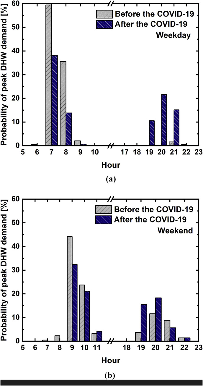
Fig. 8 shows the probability of the peak DHW demand appears during weekdays (a) and weekends (b) before/after the COVID-19 pandemic. During weekdays, the number of days when peak demand occurred between 07:00 and 09:00 before the COVID-19 pandemic accounted for 95.01%. However, the ratio of days when peak demand occurs during the same time after the COVID-19 pandemic accounted for only 51.97%, which indicated a large difference from before the COVID-19 pandemic. The ratio of days when peak DHW demand occurred between 19:00 and 22:00 after the COVID-19 pandemic largely increased from 2.27% to 47.37%. This seems to be because of the distribution effect of demand because of the decreased amount of DHW used in the morning, as mentioned previously.
Fig. 8.
Probability of the peak DHW demand during (a) weekdays and (b) weekends before/after the COVID-19.
When quantitatively looking at the distribution effect of demand, 10.96% of daily demand was used during peak time on weekdays before COVID-19. However, 7.68% of daily demand was used during peak time after COVID-19, which indicated the distribution effect was 3.28%p. Like the previously conducted analysis, during weekends, 7.85% and 7.57% of daily demand were used during peak time before and after COVID-19. Thus, it did not show considerable difference compared to weekdays.
Through the comparative analysis of data acquired before and after COVID-19, it was identified that the daily DHW demand pattern rapidly changed after the COVID-19 pandemic. However, despite the same COVID-19 pandemic situation, DHW demand pattern can be different depending on factors such as the effects of the severity of COVID-19, the government's policy, and vacation or school closing. Thus, expressing each daily DHW demand pattern as “a representative single value” could allow both identifying daily demand pattern changes based on timeline at once and allow comparing the abovementioned factors. Therefore, we used the kernel principal component analysis (KPCA) [27] to represent the daily DHW demand pattern as single number between −1 and 1. Principal component analysis (PCA) [28] is a method of converting high-dimensional data into low-dimensional data by extracting principal components (PC), which can provide the explanation of distribution in high-dimensional data. KPCA used in this study is kernel methods-applied PCA. KPCA method is described in the reference in detail [27].
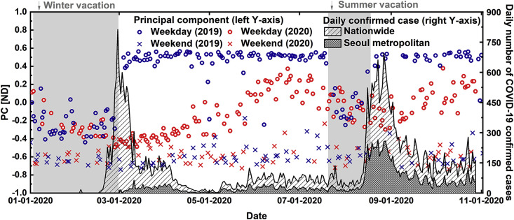
In this study, PC was extracted from the DHW demand pattern data for assessing the impact of COVID-19. Fig. 9 shows the comparison between daily PC values of 2019 (blue circle for weekdays and blue cross for weekends) and 2020 (red circle and red cross). In 2019, which was before the COVID-19 pandemic, the distribution of weekdays and weekends were clearly distinguished. Usually, PC in weekends located between −0.5 and −0.8, and PC in ordinary weekdays except school vacation season located between 0.4 and 0.6. Moreover, during the summer and winter school vacation, PC located between weekdays and weekends rather than having values of weekdays. Because of the different starting and ending dates of vacations for each school (elementary, middle, high and university), there were gradual falling and rising trends of PC in weekdays. However, there was considerable increase of PC in weekdays on March 2nd because all schools began the semester on the same day.
Fig. 9.
The principal component of 2020 and changes in the trend of new confirmed cases.
When examining the weekends’ tendency in 2020, the PC was located almost in the same area with 2019, which is consistent with the result of previously conducted statistical analysis. The PC values of weekdays showed a similar tendency to 2019 until mid-February, which was before the COVID-19 emerged but began to show difference with 2019 after the emergence of patients. In particular, the first wave began late February, which led to the closing of schools, a sharp difference with 2019 occurred, and the PC values of weekdays came close to the weekend area. As the increase in the number of the COVID-19 patients showed a stable trend, it showed a tendency to gradually recover to the PC area before the first wave, and which located the same PC area during the summer vacation as before the COVID-19 pandemic. The difference emerged again as the second wave started after late August.
The right y-axis of Fig. 9 shows changes in the trend of the number of new daily COVID-19 confirmed cases. When the number of new confirmed cases rapidly increased, the PC difference was increased between 2020 and 2019. After that, PC tended to return to the ordinary PC level in 2019 as the number of new confirmed cases decreased slowly. This phenomenon was repeatedly observed in all the two waves.
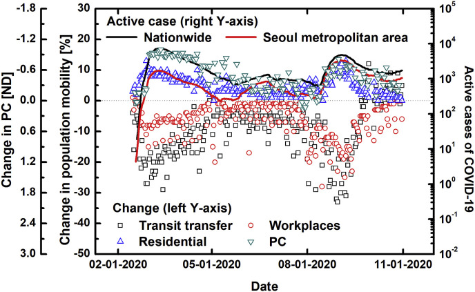
To analyze the causes of changes in the daily DHW demand pattern, deriving variables related to COVID-19, which can reflect changes in the life patterns of people is necessary. The first y-axis on the left side of Fig. 10 shows changes in the population mobility in transportation, workplaces, and residential areas during the COVID-19 pandemic period compared to the period before the pandemic, which was revealed by Google Community Mobility Reports [29]. The population mobility is attributed to counting the number of people staying in the corresponding places and comparing it with the previous result. More people stayed in the places than in the period before the COVID-19 pandemic if this value is more than 0 and less people stayed in the places if it is less than 0. The second y-axis on the left side of Fig. 10 shows the changes in the PC of the DHW demand pattern before and after the COVID-19 pandemic. After the COVID-19 pandemic, the utilization of public transportation and the ratio of time spent for staying at workplaces were largely decreased, whereas time spent for staying at homes was increased. As previously mentioned, the DHW demand was increased because residents were able to stay at homes longer because of causes such as working from home and delay in school opening. Furthermore, there was a large change in PC of DHW demand pattern after the COVID-19 pandemic. The y-axis on the right side of Fig. 10 shows the daily changes in the active cases of COVID-19 on a log scale. Generally, the active case is defined as the number of accumulated COVID-19 confirmed cases subtracted by the number of recovered patients and casualties [30]. Currently, this refers to the number of patients who are infected with the COVID-19, and the active cases were indicated separately for the entire country and the Seoul metropolitan area (where our study site is located). An interesting part is that the changes in both population mobility and the PC of the DHW demand pattern show a similar tendency to the trend of active cases. In both February and September, when the number of active cases rapidly increased, changes in population mobility in public transit transfer, workplaces, residential areas, and DHW demand pattern PC showed their peak, thus showing a similar tendency to that of active cases. Furthermore, when the number of active cases slowly reduced, the changes in population mobility and DHW demand pattern PC were recovered to the level of the previous year. In other words, the number of active cases of COVID-19 can effectively reflect changes in the life patterns of people because of the pandemic. Population mobility data are a good indicator to use in the prediction model; however, Google and Apple are temporarily allowing to share these data because of the pandemic; these data can be limited at any time. However, the number of active cases is the open-source information that anyone can collect. Thus, active cases can be useful in comparing the life pattern changes with energy demand pattern in the future case of any other epidemic outbreak.
Fig. 10.
Changes in the trends of PC, population mobility, and active cases of COVID-19.
4. Predictive analysis of the impact of COVID-19 in DHW demand
4.1. ANN model development
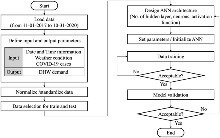
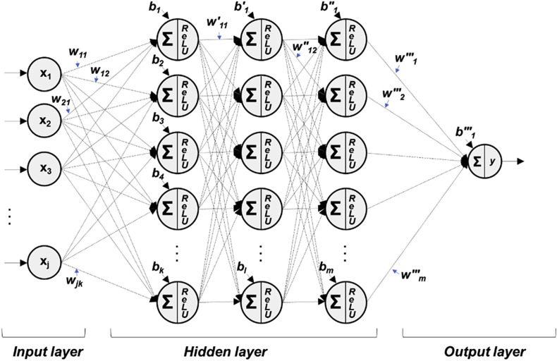
From Chapter 3, the DHW demand and changes in its pattern after COVID-19 were investigated with acquired demand data before and after the pandemic. To specifically identify and analyze the effects of COVID-19 on DHW demand, having an analysis model that reflects the correlation between COVID-19 and DHW demand is necessary. For this purpose, an ANN model that is developed and established based on the actual DHW demand to understand the effects of COVID-19. The ANN is one of the machine learning models inspired by simulating physical signals and the neuron system of the human brain. The ANN model allows to solve physical phenomena or engineering problems without a clear equation [[31], [32], [33], [34], [35], [36], [37]]. Fig. 11 shows the flowchart for the development of ANN model algorithm. The model used in this study was designed to predict hourly DHW demand through inputs such as climate, time, and COVID-19 information. Fig. 12 and Table 3 show the schematic and structure of this analysis model, respectively.
Fig. 11.
Flowchart of ANN model algorithm.
Fig. 12.
Structure of the ANN predicting DHW demand.
Table 3.
Summary of the ANN model.
| Neural network information | ||
|---|---|---|
| Input | Outdoor temperature [oC] | Hourly average value |
| City water temperature [oC] | Measured value | |
| Month | 1–12 | |
| Day | 1–31 | |
| Hour | 0–23 | |
| Day of the week | 1(Sunday) – 7(Saturday) | |
| Holiday | 0(non-holiday), 1(public holyday), 2(new-year's day, Thanksgiving Day) | |
| Consecutive holiday | The number of weekends or holidays out of the five days, including the day and two days before and after | |
| Active case in nationwide | log10(active case in nationwide area), 0 at no active case | |
| Active case in Seoul metropolitan | log10(active case in Seoul metropolitan area), 0 at no active case | |
| Output | DHW demand [MWh] | Measured value |
| Number of hidden layers | 3 | |
| Number of neurons in a hidden layer | 100 | |
| Activation function | ReLU | y = max (0, x) |
| Train-test data ratio | 7:3 | |
| Standardization | Z-score standardization | x' = (x − μ)/σ |
This model is composed of an input layer, a hidden layer, and an output layer. The input layer plays a role of processing factors that affect DHW demand such as climate, time, and the COVID-19 information to suit a machine learning model, and the number of neurons is same as the input values. The hidden layer plays a role of representing the relationship between input and output values by reflecting the degree of influence between adjacent neurons. Lastly, the output layer plays a role of outputting the calculation result (hourly DHW demand) of the hidden layer by processing it properly.
To accurately predict the DHW demand, designing the type and form of input values that affect DHW demand is important. This model uses climate, time, and COVID-19 as input parameters, which are the main factors affecting DHW demand. The climatic information was composed of the outdoor and city water temperature. For time information, factors such as month, date, time, days, the presence of weekends, and the number of consecutive holidays were used as input values. This is because DHW demand shows different consumption characteristics by weekdays/weekends and each hour. As shown in Table 3, the days were each indicated as a number between 1 and 7, and the presence of holidays was indicated as a number between 0 and 2. The consecutive holidays in input refers to the total number of holidays or weekends within five days, which includes two days before and after the corresponding date (0–5). As shown in Fig. 9, Fig. 10, COVID-19-related information used two input values: active cases in the nationwide and in the Seoul metropolitan area, which clearly reflect the life patterns of people.
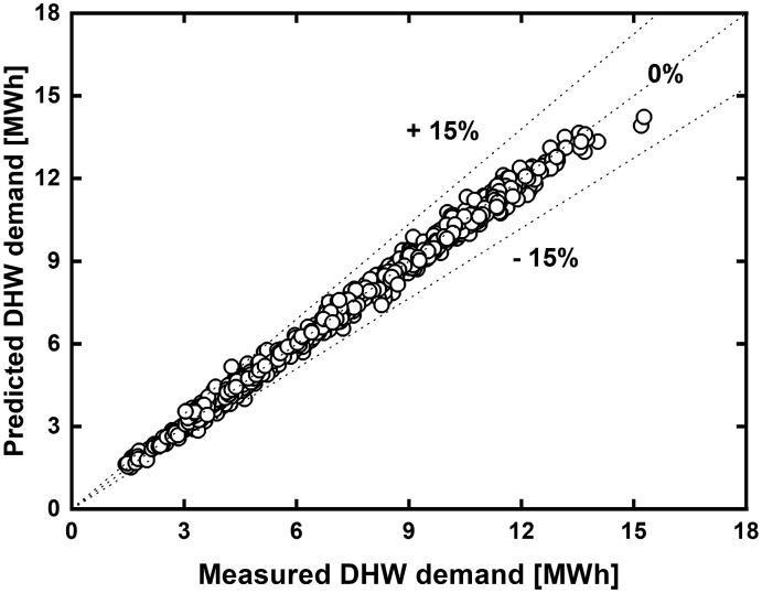
This model can be expressed as a mathematical equation, as shown in Eq. (3). The certain neuron value is calculated by multiplying the weight factor value to the previous neuron value and adding bias to the sum of these and applying an activation function. Rectified linear unit (ReLU) function was used as the activation function, as well as to increase learning accuracy, Z-score standardization was applied to input and output. The weight factor and bias between neurons in this model were calculated by the backpropagation algorithm with 70% of the randomly extracted data, and the remaining 30% of the data was used to confirm the accuracy of the model. The accuracy of this model is indicated in Table 4 , and Eq. (4) – (11) were used for each accuracy. Fig. 13 shows a comparison between the measured values of the actual daily DHW demand and the predicted values of this model. The results showed that 96.97% of the entire data had the error range of ±10% and 99.62% had the error range of ±15%.
| (3) |
| (4) |
| (5) |
| (6) |
| (7) |
| (8) |
| (9) |
| (10) |
| (11) |
Table 4.
Accuracy of the ANN model: Hourly DHW demand prediction.
| Prediction accuracy | Value |
|---|---|
| R2 | 0.9749 |
| RMSE | 0.0311 |
| CV(RMSE) | 10.348% |
| MBE | 0.374% |
| MAE | 0.0212 |
| MSLE | 0.0005 |
| COV | 0.0515 |
| Correlation | 0.9893 |
Fig. 13.
Comparison between the actual daily DHW demand and daily DHW demand predicted by the model.
4.2. Impact of COVID-19 in DHW demand
Variations in DHW demand because of changes in input values can be estimated through the machine learning model developed in this study. For example, fixing all input conditions (e.g., outdoor temperature, city water temperature, and climatic information) while changing the number of the COVID-19 active cases will indicate changes in DHW demand caused only changes in the number of the COVID-19 patients under the same condition for all external environmental condition or climatic information.
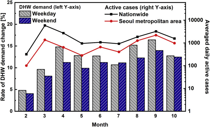
Fig. 14 shows the rate of increase in monthly DHW demand because of the COVID-19 pandemic and trend changes in active cases. While Fig. 6 simply compared DHW demand before and after COVID-19 for the rate of increase in DHW demand, Fig. 14 shows the model simulation difference between the actual DHW demand after COVID-19 as well as a case assuming no COVID-19 patients (active case = 0) during the same period under the same climatic condition. Because all other conditions (e.g., climatic and time information) are same, the rate of increase in DHW caused solely by COVID-19 (excluding other factors) can be shown. After the COVID-19 pandemic, DHW demand increased by 8.08%–16.41% each month (excluding February when the COVID-19 started), and the increased number of active cases led to increased DHW demand. Therefore, it presented that the rate of increase in DHW demand and active cases are closely related. Moreover, COVID-19 caused a greater increase in DHW demand during weekdays than weekends because of lifestyle changes in workplaces, schools, and outdoor activities during weekdays. DHW demand during the weekends increased because of factors such as reduction in the frequency of going out and the increased importance of hygiene. Comparing Figs. 14 and 6, COVID-19 active case changes affected 12.72%/11.22% (weekday/weekend) increase in June and 15.20%/12.27% increase in August; however, in reality, 2.13%/11.75% decrease in June and 58.98%/56.83% increase in August. This result can be explained because of the greater impact of city water temperature changes at that time. Therefore, predicting the accurate DHW demand requires careful consideration of climatic information and changes in COVID-19 active cases.
Fig. 14.
The rate of increase in monthly DHW demand caused by the COVID-19 pandemic and changes in the trend of active cases for each month.
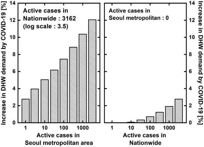
Fig. 15 analyzed the changes in DHW demand as per the range and scale of COVID-19 active cases. For this purpose, we compared DHW demand predictions using model variables as (1) the active cases of Seoul metropolitan area where the study site locates and (2) the active cases of nationwide. The result shows that DHW demand increased steadily when the active cases in Seoul metropolitan area were increased and those in the nationwide were fixed. However, when nationwide active cases increased sequentially while active cases in the Seoul metropolitan area were fixed, and the increase range was lower although it showed a linear increase. These results show that the increasing prevalence of COVID-19 in areas where people reside is more sensitive than the nationwide spread trend, thus affecting DHW demand. Moreover, this indicates that rather than considering the nationwide trend of active case growth, reflecting the situation in the region is more necessary for predicting DHW demand.
Fig. 15.
Changes in the rate of increase in DHW demand caused by changes in active cases in the Seoul metropolitan area and nationwide.
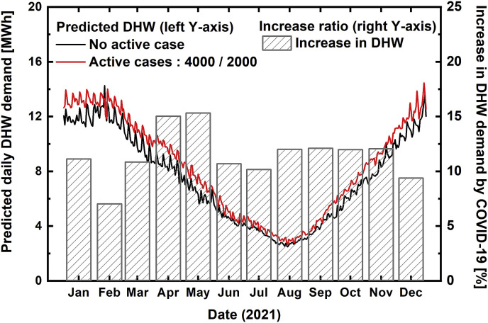
Fig. 16 shows the prediction of the rate of increase in DHW demand in 2021 due to COVID-19 by the ANN model. The climatic condition of 2021 was assumed as the average level of the past (the average level of the past three years), and the numbers of active cases nationwide and in Seoul metropolitan area were assumed as 4000 and 2000, respectively. Through the model, annual DHW demand will increase by ∼11.19% if the number of active cases is maintained at 4000 people, and it indicated an almost consistent rate of increase in monthly DHW demand. Based on the characteristics of changes in DHW demand because of changes in the number of active cases, which was derived through the above analysis, a correlation was developed to derive the rate of increase in DHW demand using the active cases. The format of the correlation is shown in Eq. (12).
| (12) |
Fig. 16.
Prediction of DHW demand using ANN model in 2021.
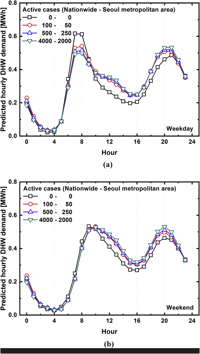
Fig. 17 shows the prediction of changes in hourly DHW demand during weekdays and weekends because of the number of active cases. In the case of weekdays, DHW demand tended to decrease as the number of active cases increased from 06:00 to 09:00, which is time for going to work and school. However, DHW demand tended to increase as the number of active cases increased from 10:00 to 15:00. Although DHW demand increased from 16:00 to 18:00, it showed a small rate of increase based on changes in the number of active cases. From 19:00 to 22:00, DHW demand tended to increase as the number of active cases increased. Although the peak time range for DHW demand before the COVID-19 pandemic was between 07:00 and 08:00, the peak gradually decreased as the number of active cases increased. When the number of nationwide active cases was more than 4000 people, the DHW demand between 20:00 and 21:00 became the maximum DHW demand peak as it surpassed the peak DHW demand between 07:00 and 08:00.
Fig. 17.
ANN model prediction for changes in hourly DHW demand during a) weekdays and b) weekends caused by changes in active cases.
For weekends, DHW demand largely increased between 09:00 and 21:00 as the number of active cases increased, but other timeslots showed no large changes. As with weekdays, weekends showed the maximum peak of DHW demand at 20:00; not in morning if the number of nationwide active cases surpassed 4000. Moreover, because of the economic downturn caused by COVID-19, “A Prolonged Sunday” (where energy consumption patterns during weekdays and weekends are assimilated) phenomenon was indicated in DHW demand in a similar form. This phenomenon was more clearly indicated as the number of active cases increased [10].
5. Conclusion
This study aimed to investigate the relationship between COVID-19 and DHW demand. For this purpose, the analysis was conducted with various factors and the influences of COVID-19 on DHW demand and developed a machine learning model with ANN to predict DHW demand after the COVID-19 pandemic. Utilizing data gathered for the past three years (November 2017–October 2020) from an apartment complex of 918 households in the Seoul metropolitan area of Republic of Korea through a smart DHW submeters, DHW demand and peak mobility caused by changes in daily life pattern based on the occurrence of the COVID-19 patients were analyzed. Based on this study, DHW demand is influenced dominantly by climate, time, and the severity of COVID-19. Furthermore, through non-dimensional analysis, KPCA and Google mobility result analyses, it was identified that the COVID-19 active cases can most properly explain changes in DHW demand and its pattern.
Based on these results, a prediction model was developed and established, which can predict hourly DHW demand through the machine learning method with ANN. It used factors such as climate, time, and the COVID-19 information, and its accuracy was R2 = 0.9749. In addition, a correlation was developed to predict the rate of increase in DHW demand based on changes in the number of active cases. The analysis result of the model indicated that DHW demand increased by 8.08%–16.41% every month after the COVID-19 pandemic, and it rapidly increased as the number of active cases increased. Moreover, DHW demand and changes in its pattern were influenced by active cases in the area belonged more dominantly compared to nationwide active cases. Furthermore, it was found that the hourly DHW demand pattern during weekdays and weekends largely shifted based on an increase in active cases, as well as a larger change in its pattern occurred during weekdays than weekends. The peak in morning gradually decreased as the number of active cases increased; it was found that if the number of nationwide active cases surpasses 4000 during both weekdays and weekends, the maximum peak of DHW demand occurs in afternoon, and not in the morning.
Credit author statement
Dongwoo Kim: Methodology, Investigation, Writing – original draft, Visualization, Validation, Taesu Yim: Methodology, Investigation, Writing, Formal analysis, Jae Yong Lee: Funding acquisition, Project administration, Supervision, Methodology, Investigation, Conceptualization, Writing – review & editing.
Declaration of competing interest
The authors declare that they have no known competing financial interests or personal relationships that could have appeared to influence the work reported in this paper.
Acknowledgments
This work was conducted under the framework of the research and development program of the Korea Institute of Energy Research (C1-2419).
References
- 1.Dubey S., Biswas P., Ghosh R., et al. Psychosocial impact of COVID-19. Diabetes Metab Syndr Clin Res Rev. 2020;14(5):779–788. doi: 10.1016/j.dsx.2020.05.035. [DOI] [PMC free article] [PubMed] [Google Scholar]
- 2.Nicola M., Alsafi Z., Sohrabi C., et al. The socio-economic implications of the coronavirus pandemic (COVID-19): a review. Int J Surg. 2020;78(March):185–193. doi: 10.1016/j.ijsu.2020.04.018. [DOI] [PMC free article] [PubMed] [Google Scholar]
- 3.Arendt F., Markiewitz A., Mestas M., Scherr S. COVID-19 pandemic, government responses, and public mental health: investigating consequences through crisis hotline calls in two countries. Soc Sci Med. 2020;265(November):113532. doi: 10.1016/j.socscimed.2020.113532. [DOI] [PubMed] [Google Scholar]
- 4.Paredes M.R., Apaolaza V., Fernandez-Robin C., Hartmann P., Yañez-Martinez D. The impact of the COVID-19 pandemic on subjective mental well-being: the interplay of perceived threat, future anxiety and resilience. Pers Indiv Differ. 2021;170(October 2020):110455. doi: 10.1016/j.paid.2020.110455. [DOI] [PMC free article] [PubMed] [Google Scholar]
- 5.Xiong J., Lipsitz O., Nasri F., et al. Impact of COVID-19 pandemic on mental health in the general population: a systematic review. J Affect Disord. 2020;277(July):55–64. doi: 10.1016/j.jad.2020.08.001. [DOI] [PMC free article] [PubMed] [Google Scholar]
- 6.Akhtaruzzaman M., Boubaker S., Chiah M., Zhong A. COVID−19 and oil price risk exposure. SSRN Electron J. 2020:101882. doi: 10.2139/ssrn.3650151. [DOI] [PMC free article] [PubMed] [Google Scholar]
- 7.Sovacool B.K., Furszyfer Del Rio D., Griffiths S. Contextualizing the Covid-19 pandemic for a carbon-constrained world: insights for sustainability transitions, energy justice, and research methodology. Energy Res Soc Sci. 2020;68(July):101701. doi: 10.1016/j.erss.2020.101701. [DOI] [PMC free article] [PubMed] [Google Scholar]
- 8.Brosemer K., Schelly C., Gagnon V., et al. The energy crises revealed by COVID: intersections of Indigeneity, inequity, and health. Energy Res Soc Sci. 2020;68(May):101661. doi: 10.1016/j.erss.2020.101661. [DOI] [PMC free article] [PubMed] [Google Scholar]
- 9.Klemeš J.J., Fan Y Van, Tan R.R., Jiang P. Minimising the present and future plastic waste, energy and environmental footprints related to COVID-19. Renew Sustain Energy Rev. 2020;127(April) doi: 10.1016/j.rser.2020.109883. [DOI] [PMC free article] [PubMed] [Google Scholar]
- 10.Global I.E.A. Energy Rev. 2020:2020. doi: 10.1787/a60abbf2-en. [DOI] [Google Scholar]
- 11.Kanda W., Kivimaa P. What opportunities could the COVID-19 outbreak offer for sustainability transitions research on electricity and mobility? Energy Res Soc Sci. 2020;68(May):101666. doi: 10.1016/j.erss.2020.101666. [DOI] [PMC free article] [PubMed] [Google Scholar]
- 12.Abu-Rayash A., Dincer I. Analysis of the electricity demand trends amidst the COVID-19 coronavirus pandemic. Energy Res Soc Sci. 2020;68(July):101682. doi: 10.1016/j.erss.2020.101682. [DOI] [PMC free article] [PubMed] [Google Scholar]
- 13.Gillingham K.T., Knittel C.R., Li J., Ovaere M., Reguant M. The short-run and long-run effects of covid-19 on energy and the environment. Joule. 2020;4(7):1337–1341. doi: 10.1016/j.joule.2020.06.010. [DOI] [PMC free article] [PubMed] [Google Scholar]
- 14.Werth A., Gravino P., Prevedello G. Impact analysis of COVID-19 responses on energy grid dynamics in Europe. Appl Energy. 2021;281(October 2020):116045. doi: 10.1016/j.apenergy.2020.116045. [DOI] [PMC free article] [PubMed] [Google Scholar]
- 15.Zhang X., Pellegrino F., Shen J., et al. A preliminary simulation study about the impact of COVID-19 crisis on energy demand of a building mix at a district in Sweden. Appl Energy. 2020;280(May):115954. doi: 10.1016/j.apenergy.2020.115954. [DOI] [PMC free article] [PubMed] [Google Scholar]
- 16.IEA. Data and statistics. https://www.iea.org/data-and-statistics
- 17.Zanocco C., Flora J., Rajagopal R., Boudet H. Exploring the effects of California's COVID-19 shelter-in-place order on household energy practices and intention to adopt smart home technologies. SSRN Electron J. 2020;(November):110578. doi: 10.2139/ssrn.3650655. [DOI] [PMC free article] [PubMed] [Google Scholar]
- 18.Cvetković D., Nešović A., Terzić I. Impact of people's behavior on the energy sustainability of the residential sector in emergency situations caused by COVID-19. Energy Build. 2021;230:110532. doi: 10.1016/j.enbuild.2020.110532. [DOI] [PMC free article] [PubMed] [Google Scholar]
- 19.Cheshmehzangi A. COVID-19 and household energy implications: what are the main impacts on energy use? Heliyon. 2020;6(10) doi: 10.1016/j.heliyon.2020.e05202. [DOI] [PMC free article] [PubMed] [Google Scholar]
- 20.Kottek M., Grieser J., Beck C., Rudolf B., Rubel F. World map of the Köppen-Geiger climate classification updated. Meteorol Z. 2006;15(3):259–263. doi: 10.1127/0941-2948/2006/0130. [DOI] [Google Scholar]
- 21.Statistics Korea . Register-Based Census ); 2019. Population and housing census. [Google Scholar]
- 22.Lee J.Y., Im Y.H. 2015. Hot water meter and measuring method thereof. [Google Scholar]
- 23.Ahmed K., Pylsy P., Kurnitski J. Hourly consumption profiles of domestic hot water for different occupant groups in dwellings. Sol Energy. 2016;137:516–530. doi: 10.1016/j.solener.2016.08.033. [DOI] [Google Scholar]
- 24.Han J., Kamber M., Pei J. 2012. Data mining: concepts and techniques. [DOI] [Google Scholar]
- 25.Fuentes E., Arce L., Salom J. A review of domestic hot water consumption profiles for application in systems and buildings energy performance analysis. Renew Sustain Energy Rev. 2018;81(April 2017):1530–1547. doi: 10.1016/j.rser.2017.05.229. [DOI] [Google Scholar]
- 26.Ulseth R., Lindberg K., Alonso M., Utne Å. Measured load profiles and heat use for “low energy buildings” with heat supply from district heating. Energy Procedia. 2017;116:180–190. doi: 10.1016/j.egypro.2017.05.066. [DOI] [Google Scholar]
- 27.Schölkopf B., Smola A., Müller K.-R. Nonlinear component analysis as a kernel eigenvalue problem. Neural Comput. 1998;10(5):1299–1319. doi: 10.1162/089976698300017467. [DOI] [Google Scholar]
- 28.Jolliffe I. International encyclopedia of statistical science. Springer Berlin Heidelberg; Berlin, Heidelberg: 2011. Principal component analysis; pp. 1299–1319. [DOI] [Google Scholar]
- 29.Google COVID-19 community mobility Reports. https://www.google.com/covid19/mobility/
- 30.Rath S., Tripathy A., Tripathy A.R. Prediction of new active cases of coronavirus disease (COVID-19) pandemic using multiple linear regression model. Diabetes Metab Syndr Clin Res Rev. 2020;14(5):1467–1474. doi: 10.1016/j.dsx.2020.07.045. [DOI] [PMC free article] [PubMed] [Google Scholar]
- 31.Ledesma S., Belman-Flores J.M., Barroso-Maldonado J.M. Analysis and modeling of a variable speed reciprocating compressor using ANN. Int J Refrig. 2015;59:190–197. doi: 10.1016/j.ijrefrig.2015.08.009. [DOI] [Google Scholar]
- 32.Zendehboudi A., Li X., Wang B. Utilization of ANN and ANFIS models to predict variable speed scroll compressor with vapor injection. Int J Refrig. 2017;74:473–485. doi: 10.1016/j.ijrefrig.2016.11.011. [DOI] [Google Scholar]
- 33.Işik E., Inallı M. Artificial neural networks and adaptive neuro-fuzzy inference systems approaches to forecast the meteorological data for HVAC : the case of cities for Turkey. Energy. 2018;154:7–16. doi: 10.1016/j.energy.2018.04.069. [DOI] [Google Scholar]
- 34.Kim D., Song K.S., Lim J., Kim Y. Analysis of two-phase injection heat pump using artificial neural network considering APF and LCCP under various weather conditions. Energy. 2018;155:117–127. doi: 10.1016/j.energy.2018.05.046. [DOI] [Google Scholar]
- 35.Peng Y., Ghahnaviyeh M.B., Ahamd M.N., et al. Analysis of the effect of roughness and concentration of Fe3O4/water nanofluid on the boiling heat transfer using the artificial neural network: an experimental and numerical study. Int J Therm Sci. 2021;163(January):106863. doi: 10.1016/j.ijthermalsci.2021.106863. [DOI] [Google Scholar]
- 36.Xu X., Liu J., Wang Y., Xu J., Bao J. Performance evaluation of ground source heat pump using linear and nonlinear regressions and artificial neural networks. Appl Therm Eng. 2020;180(August):115914. doi: 10.1016/j.applthermaleng.2020.115914. [DOI] [Google Scholar]
- 37.Faegh M., Behnam P., Shafii M.B., Khiadani M. Development of artificial neural networks for performance prediction of a heat pump assisted humidification-dehumidification desalination system. Desalination. 2021;508(February):115052. doi: 10.1016/j.desal.2021.115052. [DOI] [Google Scholar]


