. 2021 May 11;10:e60988. doi: 10.7554/eLife.60988

Figure 2. The evolution of choice in human premotor cortex.

(A) Dorsal premotor cortex (PMd) was the a priori region of interest for this study. Indeed, using source localization and a contrast between trials containing any input or response adaptation, compared to no adaptation, revealed a cluster involving M1 and left PMd (group contrast, whole-brain cluster-level FWE-corrected at p<0.05 after initial thresholding at p<0.001; PMd peak coordinate: x=-37, y=-6, z = 55). Importantly, this contrast was agnostic and orthogonal to any differences between input and response adaptation, relevant and irrelevant input adaptation, or pre- vs. post-training effects (including any timing differences, as beamforming was performed in the time window [−250, 750] ms). (B) The time-resolved nature of magnetoencephalography (MEG), combined with a selective suppression of different choice features, allowed us to track the evolution of the choice on a millisecond timescale. Linear regression coefficients from a regression performed on data from left premotor cortex (PMd) demonstrate an early representation of context (motion or colour) and switch (attended dimension same or different from TS) from ~8 ms (sliding window centred on 8 ms contains 150 ms data from [−67,83] ms). The representation of inputs, as indexed using repetition suppression (RS), emerged from around 108 ms (whether or not the input feature, colour, or motion was repeated). Finally, the motor response, again indexed using RS (same finger used to respond to adaptation stimulus [AS] and test stimulus [TS] or not), and TS choice direction (left or right, unrelated to RS) were processed from 275 ms. *p<0.001; error bars denote SEM across participants; black line denotes group average. (C) The distribution of individual peak times across the 22 participants directly reflects this evolution of the choice process. In particular, it shows significant differences in the processing of input and response, consistent with premotor cortex transforming sensory inputs into a motor response.

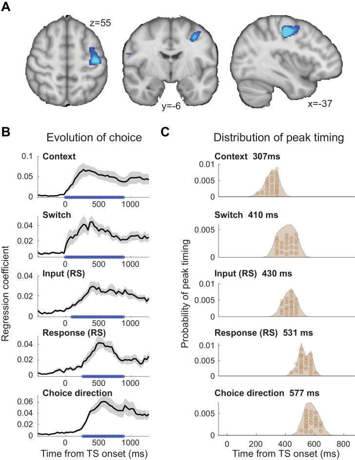
Figure 2—source data 1. Contains 'pre' and 'post' [Time x Regressors x Subjects] for Figure 2B.
Figure 2—source data 2. Contains 'dat' [Regressors x Subjects] for Figure 2B.

Figure 2.

Figure 2—figure supplement 1. Premotor cortex processes choice inputs and outputs.

Figure 2—figure supplement 1.

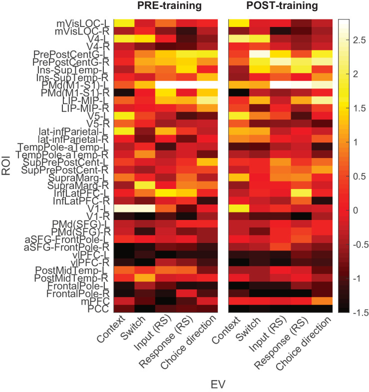
Dorsal premotor cortex (PMd) was the a priori region of interest for this study. As shown in Figure 2A, beamforming for source localization identified a cluster involving left PMd from a contrast probing any input or response adaptation across both pre- and post-training sessions. Here we show an additional parcellation into 38 regions using beamforming, which confirmed that the linear regression coefficients for both input and response suppression were strongest in the parcel containing premotor cortex (PMd(M1-S1)-L). Colours denote the maximum linear regression coefficient in the range [−500,1150] ms. Unlike in Figure 6, this analysis used the same regressors used to examine PMd responses in Figures 24, with input and response regressors capturing repetition suppression effects.
Figure 2—figure supplement 1—source data 1. Contains 'pre' and 'post' [ROIs x Regressors].
Figure 2—figure supplement 2. Simulations show sufficient parameter recovery given the experimental design.

Figure 2—figure supplement 2.

To test whether we could recover linear regression coefficients using the same design matrix as used in the experiment, we first simulated magnetoencephalography (MEG) signals using y = Xb + εp, where y is a vector of size T × 1, X is the design matrix of a specific subject in the experiment of size T × M, b is the vector of true linear regression coefficients of size M × 1, T is the number of trials, M is the number of regressors, ε is Gaussian noise drawn from N(0,1), and p is the noise multiplication factor. We set b, the true linear regression coefficients to [250, 150, 100, 150, 150, 200]. These are analogous to the six regressors in the main analyses (Context, Relevant adaptation [RelvAdpt], Irrelevant adaptation [IrrelAdpt], Response adaptation [RespAdpt], Switch, and Choice). We varied the noise multiplication factor between [1, 5, 50]. We used a regularized regression to mimic the regression procedure used for the real data. We varied the regularization term (λ) between [0.00001, 0.00005, 0.0001, 0.0005] and used the optimal one in each case. We repeated this analysis for all subjects and averaged the estimated linear regression coefficients across subjects. We found that for all noise levels (A for p=1 [λ = 0.00001]; B for p=10 [λ = 0.0001]; C for p=50 [λ = 0.0005]), we could accurately recover the true values. The horizontal line indicates the median. The bottom and top edges of the box indicate the 25th and 75th percentiles, respectively. The circles denote outliers and the whiskers extend to the most extreme data points not considered as outliers.
Figure 2—figure supplement 2—source data 1. Contains 'a_est', 'b_est', 'c_est' [Subjects x Regressors], and 'betas_true' [Regressors x 1].
Figure 2—figure supplement 3. Simulations show sufficient independence between estimated linear regression coefficients.

Figure 2—figure supplement 3.

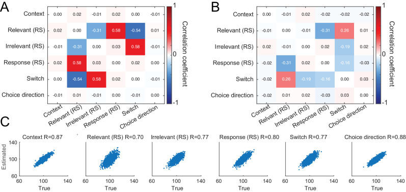
In addition to showing sufficient parameter recovery (Figure 2—figure supplement 2), we probed the correlation among estimated linear regression coefficients. Even if the true coefficients were not correlated, estimated coefficients may show artificial dependencies due to correlations present in the design matrix. To investigate this possibility, we generated synthetic data using y = Xb + ε∗p, as before. This time, we set all values in b to the same value of 100. Critically, we added Gaussian noise drawn from N(0,5) to each linear regression coefficient separately. We repeated this procedure 100 times for each subject and calculated the correlation between estimated linear regression coefficients for the five regressors within a given subject. We set p and λ to 50 and 0.0005, respectively, as in the previous simulation. We averaged obtained correlation matrices across all subjects. We found that the correlation across estimated linear regression coefficients (B) was lower than expected, given correlations present in design matrix (A). Again, we confirmed that linear regression coefficients were recoverable for all regressors (C; scatter plots showing results from all subjects; R corresponds to Pearson’s R between estimated and true linear regression coefficients).
Figure 2—figure supplement 3—source data 1. Contains 'a', 'b' [Regressors x Regressors], 'c_betas_true' and 'c_betas_pred' [Repetition x Regressors x Subjects].