Semi-Supervised Classification of Noisy, Gigapixel Histology Images

Abstract

One of the greatest obstacles in the adoption of deep neural networks for new medical applications is that training these models typically require a large amount of manually labeled training samples. In this body of work, we investigate the semi-supervised scenario where one has access to large amounts of unlabeled data and only a few labeled samples. We study the performance of MixMatch and FixMatch–two popular semi-supervised learning methods–on a histology dataset. More specifically, we study these models’ impact under a highly noisy and imbalanced setting. The findings here motivate the development of semi-supervised methods to ameliorate problems commonly encountered in medical data applications.

I. Introduction

Convolutional Neural Networks (CNN) have been the dominant framework in many computer vision tasks. The computing resources needed to train large scale CNN have become increasingly cheaper and more democratized as the barrier to train custom deep neural networks is lowered. Today, some of the larger costs have now come from activities relating to the annotation of datasets for training and evaluating these models. These costs are exacerbated in the field of medicine where experts’ time is costly. This presents a high obstacle to apply fully-supervised machine learning techniques that requiring well-curated and fully annotated datasets.

In order to circumvent a fully-supervised model, researchers turn to techniques like semi-supervised learning (SSL) to minimize the annotation requirements to build comparable models. These learning techniques adapt to an environment where one has a small amount of labeled data and a larger proportion of unlabeled data. Recently, there has been a surge in state-of-the-art performance in semi-supervised learning using MixMatch [1] and FixMatch [2]. Both techniques rely on pseudo-labeling (guessing unknown labels for training) and data augmentation to tackle semi-supervision; however, they diverge on the manner in which they perform these procedures.

Although these methods are empirically successful in general computer vision SSL tasks, they have not been examined under conditions common in the field of histology where we find high class imbalances, and noisy samples. In this study, we explore the performance of FixMatch and MixMatch on a semi-supervised histological setting. The contribution of this work is two fold: Firstly, we apply modern SSL methods on the task of detecting disease patterns by training a multi-class model using only a few labeled images while leveraging the use of a larger amount of unlabeled images. For our use case, we will be applying SSL methods on a histology dataset especially curated for the purpose of detecting esophogeal cancer’s precursors: dysplasia, Barrett’s, and squamous tissue. Lastly, we will study the effects of imbalanced datasets on the two SSL methods.

A. Common characteristics of histology datasets

This section details some of the characteristics typical of biopsy imaging relative to generic computer vision datasets (e.g. ImageNet [3] and MS-COCO [4]).

1). Gigapixel size images:

Digitized biopsy slides are high resolution images that are much larger than standard images. These high resolution sizes are prohibitive for the application of neural networks as 1) resizing these images would destroy microscopic patterns important to the diagnosis, and 2), if resizing was not performed, off-the-shelf GPUs do not carry enough memory to store the parameters of a large model required by a gigapixel-sized input.

To ameliorate this problem, the common practice is to perform “patching” operations by subdividing the slide images into smaller patches–cropped in a sliding window manner–and use them as input data to the CNN. These patches should be small enough to fit into GPU memory and have enough visual details to carry patterns present in diseases. This method has perform well on disease detection on biopsy slides [5]-[10].

2). Open-set noise:

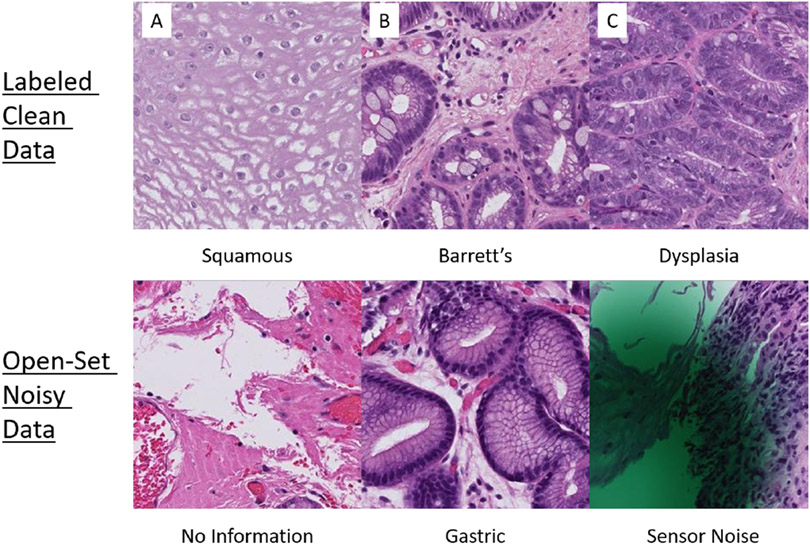
Open-set noise are areas in the biopsy containing tissue structures that are not relevant to the context of the problem. These areas could be caused by sensor noise, imperfections in the staining process, tissue outside the context of the task, etc. They are called open-set noise because these portions of the biopsy are outside the set of classes in question, yet they are still presented as training data to the model. For our use case, Figure 1 show some examples of open-set noise as compared to clean samples. In the case where a high number of open-set patches is present in the training data, CNNs will inadvertently overfit to these images [11] and may learn the wrong patterns; thus, degrading the generalizability of the model.

Fig. 1.

A) An example of normal squamous tissue of the esophagus, identified by flat, stratified cells. B) An example of nondysplastic Barrett’s esophagus, characterized by large white goblet cells filled with mucus and ovoid glands reminiscent of intestinal tissue. C) An example of dysplasia of the esophagus in which nuclei become more prominent with varying sizes and shapes (pleomorphism) and glands become more crowded. The bottom three examples are instances of open-set data which are data points that do not belong to any of the three classes in-question. They can include patches that add no information, tissue of a different type (e.g. gastric and muscular tissue), and areas of the image that contain sensor noise.

3). Imbalanced datasets:

More often than not, real-world datasets have classes that are underrepresented in the sample size relative to others. This is especially true with medical datasets where some diseases are rare and collecting more data is difficult. When trained on highly imbalanced datasets, a classifier has a tendency to pick up the patterns of the most popular classes and ignore the least popular ones–having a negative impact on its performance.

II. Related Works

This section first introduces the pertinent SSL literature within the general and medical setting. While our work primarily inspects the performance of FixMatch and MixMatch, it is related to other fields of research, including semi-supervised learning, open-set noise robustness, and class imbalance.

A. Semi-supervised Learning

Several works have explored the use of SSL on histology images. Lu et al. [12] used a two-stage approach using self-supervised contrastive learning and a multi-instance attention module to the task of binary classification of breast cancer histology images. However, their approach was evaluated on a well-curated dataset [13]. Peikari et al. [14] used a “cluster-then-label” approach finding high density areas of unlabeled clusters then using these clusters to train an SVM to learn a decision boundary through low density areas. This approach used a bag-of-words descriptor to represent each patch.

MixMatch [1] and FixMatch [2] are two deep learning methods that use ideas of consistency regularization. Consistency regularization is a constraint that forces models to produce “consistent” predictions despite applying various transformation. More specifically, in the semi-supervised setting, an unlabeled example must adhere to a single class no matter how a sample is augmented. Techniques using consistency constraints either focus on enforcing multiple identical models with varying weights to adhere to a single one-hot label [15], [16] or focus on learning a model robust against adversarial transformations [17]. Key differences between MixMatch and FixMatch methods will be detailed in Sections III-A and III-B.

B. Open-set Noise

Open-set noise recognition is a rich research area in the field of machine learning [18]. Our work closely relates to Wang et al. [19] which learns a model despite the presence of significant open-set noise by first detecting noisy samples iteratively and using a contrastive loss to learn a metric that pushes noisy samples away from clean samples in a metric space. However, Wang et al. only learns from a fully-supervised setting.

Although, STL-10 [20]–one of the benchmark datasets used to evaluate SSL techniques–contains some amount of open-set samples, the dataset’s open-set samples still have features similar to the classes in question. More specifically, the dataset’s samples belongs to one of 10 animal (e.g. dog, cat, etc.) or vehicle (e.g. car, truck, etc.) classes. However, their open-set samples only contain similar looking animals (e.g. bears, rabbits, etc.) and vehicles (e.g. trains, buses, etc.), thus having features similar to the closed-set classes. We argue that this difference between the open-set and the classes in question do not differ enough compared to histology datasets.

C. Class Imbalance

Researchers have used different approaches to tackle class imbalances like class-sensitive losses [21]-[24] and transfer learning approaches [25], [26]. FixMatch and MixMatch, through their respective augmentation schemes, more closely relates to re-sampling methods by generating synthetic data. These SSL methods’ augmentation schemes were not intended to be an approach to tackle class imbalances; however, they have the effect of generating more synthetic data. For example, one of MixMatch’s augmentation scheme MixUp [27] closely matches techniques like Synthetic Minority Oversampling Technique (SMOTE) and its variants [28]-[31] which aims to generates minority samples by selecting two examples that are close in the feature space, and synthetically sampling a linearly interpolated data point between the two examples. To the best of our knowledge, there has not been a study that addresses class imbalances in the SSL setting.

III. Methods

For this section, we will provide a brief description of MixMatch and FixMatch. Primarily, we will address the differences between their pseudo-labeling, data augmentation, and unlabeled sample loss function. We will then provide a description of the collection and processing of the esophageal dataset for our experimental analysis.

A. MixMatch

Although simple to implement, MixMatch has achieved noteworthy results on benchmark computer vision datasets. For pseudo-labeling, MixMatch infers labels by averaging the probabilities of various transformations applied to an unlabeled sample (e.g. simple horizontal and vertical rotations). This average probability score is then accentuated using a “sharpening” procedure where it increase the score of the higher class probabilities and dampen the scores of the lower class probabilities. The intuition is that if the model, on average, finds that a patch is of a certain class despite multiple transformations then the best guess label of this patch is the class with the highest probability. Thus, sharpening this score increases the confidence that a patch belongs to a certain class, and it is used as the label for training.

For data augmentation, MixMatch applies an procedure called MixUp [27] on pairs of labeled or unlabeled samples to generate more synthetic data by performing a pixel-level interpolation between images and a pairwise interpolation between class probability distributions. This synthetic data, along with their interpolated pseudo-labels, are used for training the CNN.

Finally, for unlabeled loss, MixMatch uses the mean squared error (MSE) as the loss for the unlabeled samples. Compared to cross-entropy loss, MSE is less punitive to prediction errors.

B. FixMatch

For data augmentation, FixMatch performs a strong and weak transformation on the unlabeled data point [32], [33]. If the model infers a weakly augmented sample to have a softmax score greater than a predetermined threshold τ, then the model considers this softmax score as the pseudo-label of the corresponding strongly-augmented image. The model is then trained on the strongly-augmented sample along with its pseudo-label of the weakly-augmented sample. For this study, we only implement FixMatch with RandAugment [33] which produces strong distortions of the image, and we fix the threshold to the default value of τ = .95.

Finally, for unlabeled loss, the softmax output of the strongly augmented data point is compared against the one-hot encoded pseudo-label using a cross-entropy loss. Compared to MixMatch’s MSE loss, cross-entropy loss severely punishes prediction errors.

C. Data

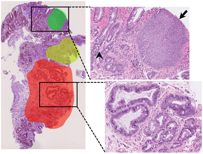
A total of 387 slide images from 133 unique patients were collected. A selection of the whole-slide image were manually annotated to highlight examples of each class (squamous, Barrett’s, and dysplasia) within each slide image (Figure 2).

Fig. 2.

Example of the annotation process on a typical whole-slide image. Red, green, and yellow highlights indicate areas that were annotated and from which labeled patches were taken. Squamous tissue (black arrow), nondysplastic Barrett’s with Goblet cells (black arrowhead), and dysplastic tissue with crowding and hyperchromasia (lower zoomed section) were all present within the same whole-slide image.

To create the labeled dataset, from 29 of the total 387 slide images, 68, 51, and 85 segments of squamous, Barrett’s, and dysplastic tissue were annotated, respectively. The segments were then subdivided into 1000x1000 pixel patches with 500-pixel overlap, and further curated to remove patches with excessive white space. All patches were extracted at the 40x magnification level. These clean samples were split at the patient-level into the labeled training dataset and testing dataset.

To create the noisy unlabeled dataset, the remaining slides were patched similar to the clean labeled set; however, no manual filtering was performed–leaving noise in the unlabeled dataset. The total training set contained 2,849 labeled patches and 889,028 unlabeled patches, and the test set contained 2,645 labeled patches (the model was blinded to these labels).

Table I summarizes the final class frequency of the dataset. Note the imbalanced nature of the dataset as the total number of dysplasia examples.

TABLE I.

Class frequency on patch-level

Type	Dysplasia	Barrett’s	Squamous	Total
Labeled Train	616	925	1,308	2,849
Unlabeled Train	-	-	-	889,028
Labeled Test	159	1365	1121	2,645

IV. Experiments

This section compares and contrasts the classification performance of the two SSL methods under various label size conditions and imbalanced settings.

A. Implementation

In all experiments, we use the ResNet-18 model. We will use the default settings for both the MixMatch and FixMatch methods, except for FixMatch’s learning rate which we set to lr = .001 (the default learning rate for MixMatch) as we have found it to converge better on the experimental dataset. For the unlabeled loss, we designated λ_u = 1 for both methods. We train both the models on 32 epochs with 512 iterations and batch size of 22 samples. The reported implementations used 1024 epochs with batch size of 64. However, we notice no increase in performance using 1024 epoch compared to 32 epochs. We used a Pytorch implementation for both FixMatch¹ and MixMatch². These implementations were verified to replicate their respective original results. Input data is resized from 1000x1000 pixels to 224x224 pixels and normalized between 0 and 1.

B. Performance Comparison

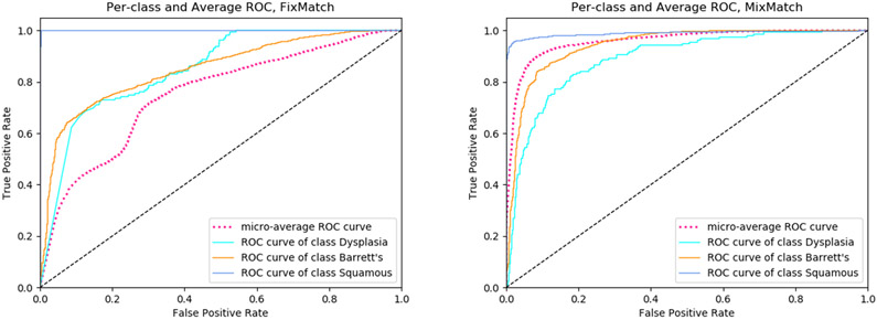
The standard way to analyze SSL methods is to measure their performance as we vary the number of labeled samples. We train FixMatch and MixMatch on two levels of labeled sample sizes: 36 and 72 patches per class; totaling 108 and 216, respectively. To test the effects of patient diversity, we also control for the number of patients from which we sample. We test 6 different patient-patch sampling combination levels: (6, 6), (4, 9), (2, 18), (6, 12), (4, 18), and (2, 36). For example, the sampling level notation (4, 9) means that we sample 4 random patients per class and, from each of these 4 patients, we sample 9 random patches. These combinations were designed such that the number of total labels were held constant to control for labeled sample sizes. We measure the average AUC and the per-class AUC for each of these combinations over 5 trials. Table II shows that MixMatch performs better than FixMatch on the average AUC and dysplasia AUC. We also see that increasing the number of patients has a bigger impact on the performance of both the models compared to just increasing the number of labeled patches, signifying that patient diversity has a larger role on the performance of these models. Figure 3 compares the performance of an identical (6, 6) patient-patch sampling on both the FixMatch and MixMatch methods.

TABLE II.

Per-class and average AUC for the esophageal Barrett’s dataset

		MixMatch
Per-class patches	(Patient, Patch)	Dysplasia	Barrett’s	Squamous	Micro-Ave.
36	(6, 6)	.91±.02	.97±.01	.99±.01	.95±.01
	(4, 9)	.89±.03	.96±.02	.99±.01	.93±.03
	(2, 18)	.83±.08	.92±.04	.98±.02	.87±.04
72	(6, 12)	.91±.01	.97±.01	.99±.01	.95±.02
	(4, 18)	.88±.05	.96±.01	.99±.01	.95±.02
	(2, 36)	.86±.03	.92±.05	.99±.01	.90±.05
		FixMatch
Per-class patches	(Patient, Patch)	Dysplasia	Barrett’s	Squamous	Micro-Ave.
36	(6, 6)	.82±.02	.74±.18	.99±.01	.73±.12
	(4, 9)	.83±.01	.88±.02	.99±.01	.80±.09
	(2, 18)	.79±.04	.80±.12	.99±.01	.73±.10
72	(6, 12)	.86±.04	.84±.13	.99±.01	.81±.13
	(4, 18)	.83±.04	.86±.06	.99±.01	.77±.09
	(2, 36)	.79±.04	.72±.16	.99±.01	.70±.08
		Full-Supervision
		Dysplasia	Barrett’s	Squamous	Micro-Ave.
All		.92±.01	.97±.01	.99±.01	.96±.01

Fig. 3.

Per-class and average ROC curve of FixMatch and MixMatch trained on a (6, 12) patient-patch combination.

As a proxy to an upper bound, we trained the model using a fully supervised method trained on all the labeled samples. The fully supervised model’s performance is comparable to MixMatch’s performance at the (6, 6) and (6, 12) combination levels, despite MixMatch only having a small fraction of the total labels.

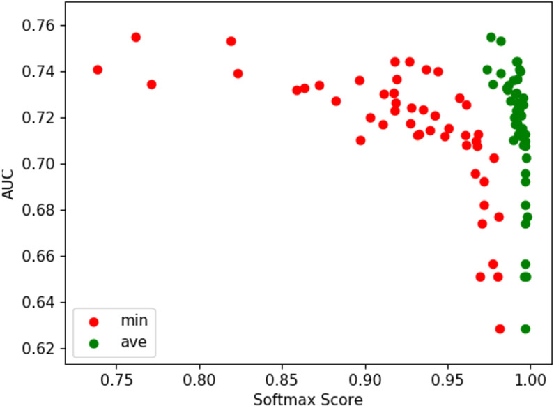
To offer an explanation as to why FixMatch produces poor results on the esophogeal dataset, we designed a follow-up experiment by tracking the effects of the softmax score of 10 hand picked, open-set examples on the AUC using the (2, 18) combination. We measure the model AUC at every 126 iterations for 64 cycles and the corresponding softmax scores that the 10 open-set examples produce. The softmax score is the probability that a given sample belongs to a certain class. Figure 4 show the minimum and average softmax scores of the last 48 cycles. This show that, as the model erroneously becomes more confident of the open-set examples, the model’s performance deteriorates as well. More interestingly, the model begins to deteriorate when the minimum softmax score exceeds .95 (FixMatch’s default threshold value).

Fig. 4.

Effects of softmax scores of 10 open-set samples on the model’s AUC for FixMatch using (2, 18) patient-patch combination.

C. Effects of Imbalances

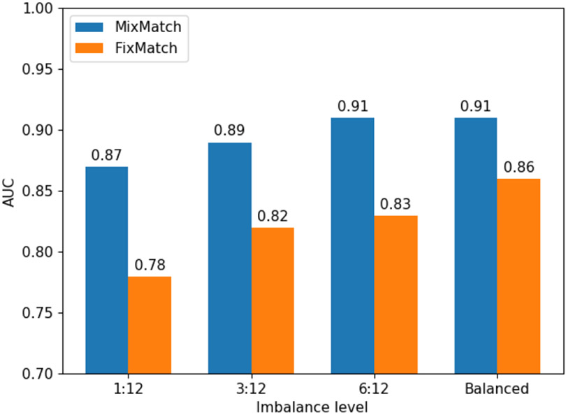
To test the effects of the various degrees of imbalances, we fix the patient-patch sampling combination at (6, 12). We then decrease the amount of labeled dysplasia samples to 1, 3, and 6 samples per patient–totaling 6, 18, and 36 samples for the dysplasia class, respectively, compared to the 72 samples for Barrett’s and squamous. We measure the average AUC across 5 trails. Table II show that MixMatch is more robust to imbalances compared to FixMatch on average. More interestingly, MixMatch has a higher average AUC on the imbalanced dysplasia class, and comparable to the balanced result at (6, 12) combination. Overall, however, both methods degrade with high level of imbalances due to their performance on the dysplasia (minority) class.

V. Discussion

This study shows a method to train a histology detection model with only a few labeled samples. With only a few exemplary images, one can train an effective model to detect esophageal disease patterns on histopathology datasets. In this study, we compare and contrast the performance of MixMatch and FixMatch. Although FixMatch performs better overall in general computer vision datasets, our results show that MixMatch performs better on histology datasets–where noisy, open-set samples are present. Also, MixMatch’s pseudo-labeling and data augmentation procedures are more robust to the impact of histology datasets, even under varying degrees of imbalanced scenarios. Finally, our experiments show that patient diversity has a significant impact on the performance of SSL methods.

While there could be many compounding factors as to why FixMatch performs poorly on datasets with open-set samples, we hypothesize that one major reason for FixMatch’s poor performance is due to its use of the thresholding method for pseudo-labeling and cross entropy loss to account for errors: the thresholding method incorrectly labels an open-set sample as one of the classes in-question and the cross-entropy loss impels the model to over-confidently predict an open-set sample as belonging to one of the classes in-question.

VI. Conclusion

This work contributes to the body of literature pertaining to SSL in medical imaging. In this study, we applied the leading SSL methods to the problem of detecting disease in histology images. We found that MixMatch performs better in the histology setting. This work also motivates the development of SSL methods that are robust to open-set noise common in histology datasets.

One weakness of this work is the lack of quantification of open-set noise; thus, future work should perform a more controlled study on the effects of noisy unlabeled samples on these methods.

Fig. 5.

Dysplasia class’s AUC score for varying levels of imbalances applied to a (6, 12) patient-patch combination. The various imbalance levels against the dysplasia class are 1:12, 3:12, 6:12, and balanced. The imbalance level 1:12 means that the dysplasia class will have 1 sample for 6 patients. And the Barrett’s and squamous class will have 12 samples from 6 patients each.

References

- [1].Berthelot David, Carlini Nicholas, Goodfellow Ian, Papernot Nicolas, Oliver Avital, and Raffel Colin A. Mixmatch: A holistic approach to semi-supervised learning. In Advances in Neural Information Processing Systems, pages 5050–5060, 2019. [Google Scholar]
- [2].Sohn Kihyuk, Berthelot David, Li Chun-Liang, Zhang Zizhao, Carlini Nicholas, Cubuk Ekin D, Kurakin Alex, Zhang Han, and Raffel Colin. Fixmatch: Simplifying semi-supervised learning with consistency and confidence. arXiv preprint arXiv:2001.07685, 2020. [Google Scholar]
- [3].Krizhevsky Alex, Sutskever Ilya, and Hinton Geoffrey E. Imagenet classification with deep convolutional neural networks. In Advances in neural information processing systems, pages 1097–1105, 2012. [Google Scholar]
- [4].Lin Tsung-Yi, Maire Michael, Belongie Serge, Hays James, Perona Pietro, Ramanan Deva, Dollár Piotr, and Zitnick C Lawrence. Microsoft coco: Common objects in context. In European conference on computer vision, pages 740–755. Springer, 2014. [Google Scholar]
- [5].Hou Le, Samaras Dimitris, Kurc Tahsin M, Gao Yi, Davis James E, and Saltz Joel H. Patch-based convolutional neural network for whole slide tissue image classification. In Proceedings of the IEEE conference on computer vision and pattern recognition, pages 2424–2433, 2016. [DOI] [PMC free article] [PubMed] [Google Scholar]
- [6].Wang Xi, Chen Hao, Gan Caixia, Lin Huangjing, Dou Qi, Huang Qitao, Cai Muyan, and Heng Pheng-Ann. Weakly supervised learning for whole slide lung cancer image classification. Medical Imaging with Deep Learning, 2018. [Google Scholar]
- [7].Tomita Naofumi, Abdollahi Behnaz, Wei Jason, Ren Bing, Suriawinata Arief, and Hassanpour Saeed. Finding a needle in the haystack: Attention-based classification of high resolution microscopy images. arXiv preprint arXiv:1811.08513, 2018. [Google Scholar]
- [8].Zhang Zizhao, Chen Pingjun, McGough Mason, Xing Fuyong, Wang Chunbao, Bui Marilyn, Xie Yuanpu, Sapkota Manish, Cui Lei, Dhillon Jasreman, et al. Pathologist-level interpretable whole-slide cancer diagnosis with deep learning. Nature Machine Intelligence, 1(5):236–245, 2019. [Google Scholar]
- [9].Courtiol Pierre, Tramel Eric W, Sanselme Marc, and Wainrib Gilles. Classification and disease localization in histopathology using only global labels: A weakly-supervised approach. arXiv preprint arXiv:1802.02212, 2018. [Google Scholar]
- [10].Chen Hanbo, Han Xiao, Fan Xinjuan, Lou Xiaoying, Liu Hailing, Huang Junzhou, and Yao Jianhua. Rectified cross-entropy and upper transition loss for weakly supervised whole slide image classifier. In International Conference on Medical Image Computing and Computer-Assisted Intervention, pages 351–359. Springer, 2019. [Google Scholar]
- [11].Zhang Chiyuan, Bengio Samy, Hardt Moritz, Recht Benjamin, and Vinyals Oriol. Understanding deep learning requires rethinking generalization. arXiv preprint arXiv:1611.03530, 2016. [Google Scholar]
- [12].Lu Ming Y, Chen Richard J, Wang Jingwen, Dillon Debora, and Mahmood Faisal. Semi-supervised histology classification using deep multiple instance learning and contrastive predictive coding. arXiv preprint arXiv:1910.10825, 2019. [Google Scholar]
- [13].Aresta Guilherme, Araújo Teresa, Kwok Scotty, Chennamsetty Sai Saketh, Safwan Mohammed, Alex Varghese, Marami Bahram, Prastawa Marcel, Chan Monica, Donovan Michael, et al. Bach: Grand challenge on breast cancer histology images. Medical image analysis, 56:122–139, 2019. [DOI] [PubMed] [Google Scholar]
- [14].Peikari Mohammad, Salama Sherine, Nofech-Mozes Sharon, and Martel Anne L. A cluster-then-label semi-supervised learning approach for pathology image classification. Scientific reports, 8(1): 1–13, 2018. [DOI] [PMC free article] [PubMed] [Google Scholar]
- [15].Laine Samuli and Aila Timo. Temporal ensembling for semi-supervised learning. arXiv preprint arXiv:1610.02242, 2016. [Google Scholar]
- [16].Tarvainen Antti and Valpola Harri. Mean teachers are better role models: Weight-averaged consistency targets improve semi-supervised deep learning results. In Advances in neural information processing systems, pages 1195–1204, 2017. [Google Scholar]
- [17].Miyato Takeru, Maeda Shin-ichi, Koyama Masanori, and Ishii Shin. Virtual adversarial training: a regularization method for supervised and semi-supervised learning. IEEE transactions on pattern analysis and machine intelligence, 41(8):1979–1993, 2018. [DOI] [PubMed] [Google Scholar]
- [18].Geng Chuanxing, Huang Sheng-jun, and Chen Songcan. Recent advances in open set recognition: A survey. IEEE Transactions on Pattern Analysis and Machine Intelligence, 2020. [DOI] [PubMed] [Google Scholar]
- [19].Wang Yisen, Liu Weiyang, Ma Xingjun, Bailey James, Zha Hongyuan, Song Le, and Xia Shu-Tao. Iterative learning with open-set noisy labels. In Proceedings of the IEEE Conference on Computer Vision and Pattern Recognition, pages 8688–8696, 2018. [Google Scholar]
- [20].Coates Adam, Ng Andrew, and Lee Honglak. An analysis of single-layer networks in unsupervised feature learning. In Proceedings of the fourteenth international conference on artificial intelligence and statistics, pages 215–223, 2011. [Google Scholar]
- [21].Lin Tsung-Yi, Goyal Priya, Girshick Ross, He Kaiming, and Dollár Piotr. Focal loss for dense object detection. In Proceedings of the IEEE international conference on computer vision, pages 2980–2988, 2017. [Google Scholar]
- [22].Shu Jun, Xie Qi, Yi Lixuan, Zhao Qian, Zhou Sanping, Xu Zongben, and Meng Deyu. Meta-weight-net: Learning an explicit mapping for sample weighting. In Advances in Neural Information Processing Systems, pages 1917–1928, 2019. [Google Scholar]
- [23].Hayat Munawar, Khan Salman, Zamir Waqas, Shen Jianbing, and Shao Ling. Max-margin class imbalanced learning with gaussian affinity. arXiv preprint arXiv:1901.07711, 2019. [Google Scholar]
- [24].Cao Kaidi, Wei Colin, Gaidon Adrien, Arechiga Nikos, and Ma Tengyu. Learning imbalanced datasets with label-distribution-aware margin loss. In Advances in Neural Information Processing Systems, pages 1565–1576, 2019. [Google Scholar]
- [25].Yin Xi, Yu Xiang, Sohn Kihyuk, Liu Xiaoming, and Chandraker Manmohan. Feature transfer learning for face recognition with underrepresented data. In Proceedings of the IEEE Conference on Computer Vision and Pattern Recognition, pages 5704–5713, 2019. [Google Scholar]
- [26].Liu Ziwei, Miao Zhongqi, Zhan Xiaohang, Wang Jiayun, Gong Boqing, and Yu Stella X. Large-scale long-tailed recognition in an open world. In Proceedings of the IEEE Conference on Computer Vision and Pattern Recognition, pages 2537–2546, 2019. [Google Scholar]
- [27].Zhang Hongyi, Cisse Moustapha, Dauphin Yann N, and Lopez-Paz David. mixup: Beyond empirical risk minimization. arXiv preprint arXiv:1710.09412, 2017. [Google Scholar]
- [28].Chawla Nitesh V, Bowyer Kevin W, Hall Lawrence O, and Kegelmeyer W Philip. Smote: synthetic minority over-sampling technique. Journal of artificial intelligence research, 16:321–357, 2002. [Google Scholar]
- [29].Han Hui, Wang Wen-Yuan, and Mao Bing-Huan. Borderline-smote: a new over-sampling method in imbalanced data sets learning. In International conference on intelligent computing, pages 878–887. Springer, 2005. [Google Scholar]
- [30].Wang Qi, Luo ZhiHao, Huang JinCai, Feng YangHe, and Liu Zhong. A novel ensemble method for imbalanced data learning: bagging of extrapolation-smote svm. Computational intelligence and neuroscience, 2017, 2017. [DOI] [PMC free article] [PubMed] [Google Scholar]
- [31].He Haibo, Bai Yang, Garcia Edwardo A, and Li Shutao. Adasyn: Adaptive synthetic sampling approach for imbalanced learning. In 2008 IEEE international joint conference on neural networks (IEEE world congress on computational intelligence), pages 1322–1328. IEEE, 2008. [Google Scholar]
- [32].Berthelot David, Carlini Nicholas, Cubuk Ekin D, Kurakin Alex, Sohn Kihyuk, Zhang Han, and Raffel Colin. Remixmatch: Semi-supervised learning with distribution alignment and augmentation anchoring. arXiv preprint arXiv:1911.09785, 2019. [Google Scholar]
- [33].Cubuk Ekin D, Zoph Barret, Shlens Jonathon, and Le Quoc V. Randaugment: Practical automated data augmentation with a reduced search space. arXiv preprint arXiv:1909.13719, 2019. [Google Scholar]