Abnormality detection and intelligent severity assessment of human chest computed tomography scans using deep learning: a case study on SARS-COV-2 assessment

Abstract

Different respiratory infections cause abnormal symptoms in lung parenchyma that show in chest computed tomography. Since December 2019, the SARS-COV-2 virus, which is the causative agent of COVID-19, has invaded the world causing high numbers of infections and deaths. The infection with SARS-COV-2 virus shows an abnormality in lung parenchyma that can be effectively detected using Computed Tomography (CT) imaging. In this paper, a novel computer aided framework (COV-CAF) is proposed for classifying the severity degree of the infection from 3D Chest Volumes. COV-CAF fuses traditional and deep learning approaches. The proposed COV-CAF consists of two phases: the preparatory phase and the feature analysis and classification phase. The preparatory phase handles 3D-CT volumes and presents an effective cut choice strategy for choosing informative CT slices. The feature analysis and classification phase incorporate fuzzy clustering for automatic Region of Interest (RoI) segmentation and feature fusion. In feature fusion, automatic features are extracted from a newly introduced Convolution Neural Network (Norm-VGG16) and are fused with spatial hand-crafted features extracted from segmented RoI. Experiments are conducted on MosMedData: Chest CT Scans with COVID-19 Related Findings with COVID-19 severity classes and SARS-COV-2 CT-Scan benchmark datasets. The proposed COV-CAF achieved remarkable results on both datasets. On MosMedData dataset, it achieved an overall accuracy of 97.76% and average sensitivity of 96.73%, while on SARS-COV-2 CT-Scan dataset it achieves an overall accuracy and sensitivity 97.59% and 98.41% respectively.

Introduction

In December 2019, a novel disease related to coronavirus family spread between several people in Wuhan, in China's Hubei Province (Chen et al. 2020). It had several clinical manifestations such as fever, cough, and dyspnea and affects the lung causing pneumonia (Chung et al. 2020). The lung becomes filled with fluid, inflamed and multiple plaque shadows and interstitial changes occur leading to Ground Glass Opacities (GGO) (Ardakani et al. 2020; Chen et al. 2020). In severe cases, lung consolidations can occur presenting a phenomenon called “white lung” (Chen et al. 2020). In March 2020, the WHO declared COVID-19, caused by Severe Acute Respiratory Syndrome Coronavirus 2 (SARS-CoV-2), to be a pandemic and a public health emergency of international concern. By November 7th, 2020, the epidemic spread to more than 200 countries with more than 49 million individuals contracted the virus worldwide and more than 1,200,000 reported deaths (WorldOmeter). There are four common methods to diagnose COVID-19 which are Reverse Transcription Polymerase Chain Reaction (RT-PCR), Computed Tomography (CT), X-ray and C-Reactive Protein Level (CPR) blood test (Fan et al. 2020). CT can play an important role in the early detection and management of COVID-19 pneumonia (Hani et al. 2020). It is more sensitive than RT-PCR and showed suggestive abnormalities even when the viral load is insufficient causing RT-PCR to produce falsely negative results (Hani et al. 2020; Long et al. 2020). It is more accurate than blood tests because some of the cases that tested by CPR blood test were tested twice as negative while the first CT test diagnosed these cases as positive (Radiopaedia). Moreover, the accuracies of CT were shown to be higher than that of X-rays as in early stages of COVID-19, a chest X-ray may be identified as normal, while CT conveys early signs of the disease (Rony Kampalath; Zu et al. 2020). In other cases of severe COVID-19, their X-ray findings may resemble that of pneumonia or acute respiratory distress syndrome (ARDS) (Rony Kampalath; Zu et al. 2020). Thus, no confident diagnosis of COVID-19 disease is possible based on chest X-ray alone (Rony Kampalath; Zu et al. 2020). In CT, advert symptoms of COVID-19 can be seen, which aids more accurate timely diagnosis compared to X-ray (Rony Kampalath; Zu et al. 2020). Timely diagnosis can lead to better prognosis, especially if the severity of the infection could be assessed on a multilevel scale. A five-level scale was introduced (Chen et al. 2020; Hani et al. 2020) (normal, early, moderate, advanced, severe) according to percentage of GGO and consolidation in lung parenchyma to help identify the risk level. Due to the increase of the COVID-19 cases worldwide, the medical system suffers from high workloads that can result into inaccurate decisions (Doi 2007; Lodwick 1966). A computer-aided diagnostic system is needed to support the medical system to detect COVID -19 infections and determine the severity degrees of these infections (Doi 2007).

In this paper, a hybrid computer-aided framework (COV-CAF), implementing a modified deep learning architecture, is proposed to detect COVID-19 infections and classify the severity of the infection based on the percentage of GGO and presence of consolidation in lung parenchyma. The model is based on fusion of automatically generated features from modified deep learning architecture with human articulated features.

The contribution of the paper can be summarized as.

• Slice selection mechanism is proposed for selection of informative candidate frames from the 3D CT-volumes

• Region of Interest (RoI) segmentation phase using unsupervised clustering is introduced.

• A modified deep learning architecture is proposed that achieved an outstanding performance in diagnosing CT compared to previously established deep learning architectures.

• A new robust hybrid machine learning system architecture is compiled (COV-CAF) for accurately diagnosing COVID-19 and its severity level. The system is based on fusion of the new proposed deep learning architecture automatic features with generated human articulated features, which noticeably improves the performance of pure deep learning architecture.

• The proposed models are validated on two benchmark datasets which are MosMedData: chest CT scans with COVID-19 related findings dataset (Morozov et al. 2020) with multi class classification of degrees of COVID-19 infections and SARS-COV-2 CT-Scan Dataset (Soares et al. 2020) with binary classes for detection of COVID-19 infections.

The paper is organized as follows: in Sect. 2, an overall literature background on using machine learning for COVID-19 disease diagnosis based on CT imaging is presented. Section 3 details the proposed system architecture and the implemented modules. In Sect. 4, a full description of the datasets used in the conducted experiments is given. Section 5 presents the experimental setup for conducting the experiments and the results of different experimental scenarios are shown and discussed. Finally, conclusions will be drawn in Sect. 6.

Related work

Automatic screening of COVID-19 through machine learning and chest scanning is a vital area of research. Chest scans directly assess the condition of the lungs (Alafif et al. 2021; Kamalov et al. 2021); thus, it can be effectively used for disease monitoring and control (Zu et al. 2020). In addition, machine learning can provide automated preliminary screening of COVID-19 saving physicians time and allowing them to focus on more critical cases (Doi 2007; Lodwick 1966). Therefore, a lot of work has been dedicated recently to study the effectiveness of applying machine learning on chest scanning for COVID-19 diagnosis. In particular, deep learning -based systems have received the highest attention.

Jaiswal et al. (2020) applied and compared a range of standard deep learning architectures for classifying COVID-19 infected patients. DenseNet201-based deep transfer learning was shown to achieve the highest accuracy of 96.25%. Ardakani et al. (2020) have extensively evaluated the performance of ten DL architectures on CT images to distinguish COVID-19 from other atypical viral and pneumonia diseases. The infection area was manually cropped and scaled with the aid of a radiologist, then input to the CNN. Transfer learning was applied to compensate for the limited dataset of size of 1020 slice. The best performance was attained by ResNet-101 with COVID-19 sensitivity of 100% and specificity of 99.02%. A similar study was conducted by Koo et al. (Koo et al. 2018) using various DL architectures to diagnose COVID-19. ResNet-50 showed the highest diagnostic performance reaching sensitivity of 99.58% and specificity 100.00%, and accuracy 99.87%, followed by Xception, Inception-v3, and VGG16. Binary classification of positive COVID 19 cases vs normal was performed by Singh et al. (2020) CNNs were applied for the classification, where the initial parameters of CNN are adjusted using multi objective differential evolution (MODE). The model achieved a sensitivity of 90% given a training to testing percentage as 9:1. The discussed systems directly applied standard classification techniques on ready to process 2D-CT slices. Nevertheless, available datasets usually require manipulation of 3D-CT volumes and/or segmentation for Region of Interest (RoI) localization.

Zhang et al. (2020) proposed a new model that starts with 14-way data augmentation techniques applied on the training set. The augmented set was input to a 7-layer CNN network with enhanced stochastic max pooling, which was used to overcome the limitations of traditional max pooling techniques. The model was used to diagnose positive COVID-19 CT infections vs normal cases and achieved sensitivity, accuracy and specificity of 94.44%, 94.03% and 93.63% respectively. Another experiment proposed by Li et al. (2020) that developed COVNet deep neural network framework for extraction of two-dimensional local and 3D global representative features. The framework included RoI segmentation using U-Net (Ronneberger et al. 2015) and data augmentation before feeding the slices into ResNet-50. The achieved sensitivity and specificity for COVID-19 were 90% and 96%, respectively. A similar approach was presented by Zheng et al. (2020), where a weakly supervised DL technique was proposed for diagnosis of COVID-19 patients using 3D CT scans. Pre-trained U-Net was also applied for segmentation of 3D lung images. The segmented regions were input to the DL architecture for prediction of infected regions. The accuracy obtained from their model was 95.9%. Another segmentation approach based on attenuation and HU value thresholding is introduced by Bai et al. (2020). In some cases, manual correction of the segmentation was performed by a radiologist. Following the segmentation phase, EfficientNet B4 was used for separating COVID-19 cases from non-COVID or other non- COVID pneumonia. The model had higher test accuracy of 96%, sensitivity of 95% and specificity of 96% compared to radiologists 85%, 79% and 88% respective values. Kang et al. (2020) adopted a traditional machine learning approach of features extraction, latent multi-view representation and classification. V-Net was used for pre-segmentation. The latent representation of the features together with Neural Network classifier reached the highest sensitivity and specificity of 96.6% and 93.2% respectively. A hybrid learning approach was investigated by Hasan et al. (2020), where the CT-slices were segmented through histogram thresholding and subsequent morphological operations. They integrated a novel Q-Deformed entropy features and DL extracted features. Long Short-Term Memory neural network was used as the classifier attaining 99.68% accuracy. Another COVID-19 model was proposed by Wang et al. (2021) to classify COVID-19 CT infection by introducing a new (L, 2) transfer feature learning (L2TFL) that was used to remove the optimal layer of pretrained CNNs before testing. A new selection algorithm was proposed to choose the best two retrained models to be fused using a deep CCT fusion discriminant correlation analysis (DCFDCA) method. The used fusion method got a better result compared to traditional fusion methods. The final model named CCSHNET achieved a micro-averaged F1 score of 97.04%.

All of the previously mentioned studies determine whether the CT scans present a negative or a positive case of COVID-19 or differentiate it from community acquired pneumonia. A step further, that is well needed, is to determine the severity of the infection and the degree of lung involvement. Hence, enable better support to the more serious cases.

Gozes et al. (2020) attempted to determine the severity of the infection using an off the shelf system to localize and provide measurements for nodules and opacities. The system was able to trace the changes in nodules and opacities size over time. However, the system was not shown to automatically classify patients based on severity level, which is a needed capability. In the work of Wang et al. (2020), a hazard value was predicted for each patient to indicate whether he/she was high or low risk. The hazard score was calculated given three prognostic features fed into Cox Hazard Proportional model.

Despite the work of Gozes et al. (2020) and Wang et al. (2020), they did not automatically detect severity levels direct from the CT scans. Thus, the automated stratification of COVID-19 severity remained under-studied, which mandates directing more efforts into this area of research.

Methods

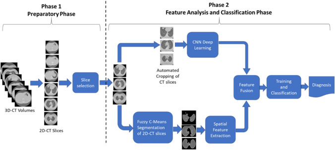
In this section, COV-CAF a robust COVID-19 Integrative Diagnostic and severity assessment system architecture is proposed to detect COVID-19 infections and classify the severity of the infection. The system consists of two main phases which are: the preparatory phase and the feature analysis and classification phase. In the preparatory phase, data preprocessing and slice selection are performed to handle the characteristics of different datasets, leading to the enhancement of image properties and improvement of the dependability of the dataset. The classification phase incorporates RoI segmentation, multi-view feature extraction and classification, which are responsible for producing an effective accurate diagnosis and severity assessment. RoI segmentation is performed using an unsupervised fuzzy clustering technique. Feature extraction is done through a hybrid technique which fuses the automatic features generated from a modified variant of an existing deep learning architecture named Norm-VGG16 (Ibrahim et al. 2020) and spatial features that are generated from the segmented RoI. The proposed system architecture is shown in Fig. 1. An illustration of each phase is presented followed by a description of each phase.

Fig. 1.

The proposed COV-CAF architecture

Preparatory phase

In this phase, a range of preprocessing steps are applied on the datasets to increase the system robustness and to limit the processing system requirements. This phase introduces two optional steps, which are Data preprocessing and Slice selection, that may be applied both or even none of them according to the nature of data used.

Data preprocessing

In case of 3D-CT volumes, the preparatory phase starts by converting the 3D-CT volumes to 2D-slices by using “med2image” library in python 3.7. The dataset volumes contain only axial view for lung as shown in Fig. 2 and all the 2D slices of each patient are saved in Joint Photographic Experts Group (jpeg) format.

Fig. 2.

2D-CT axial view

Slice selection

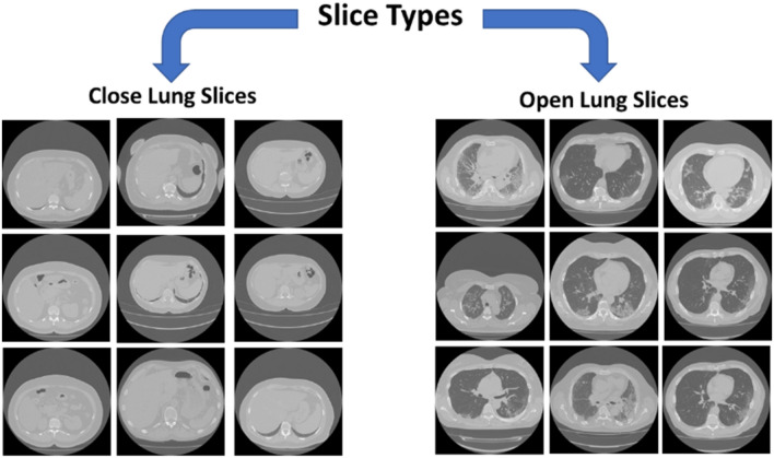
Converting 3D-CT Volumes to 2D slices generates open and closed lung slices as shown in Fig. 3. Open lung slices refer to slices with lung parenchyma, while closed lung slices contain mainly bones. The reason of conversion to 2D slices is to efficiently select the correct candidate slices with infections from all slices in 3D image sequence (Hamadi and Yagoub 2018; Rahimzadeh et al. 2020). Slice selection is used to select the informative slices (open lung slices) and reject the remaining slices, which shall positively affect training time, model accuracy and precision to generate an efficient classification model (Hamadi and Yagoub 2018; Rahimzadeh et al. 2020). An automatic slice selection technique is needed to speed up slice selection stage to save a lot of time and effort in comparison to manually selecting the desired open lung slices based on medical expert decisions (Rahimzadeh et al. 2020).

Fig. 3.

Open lung slices vs closed lung slices

Automated slice selection is proposed to separate open lung slices from closed lung slices. In the slice selection process, Histogram of Oriented Gradient features (HOG) descriptors are extracted from the CT images. Then, a subset of 2000 images of size 180 × 180 equally divided between open lung slices and closed lung slices is labeled. The labeled images are used to train SVM classifier. The remaining images are labeled using the trained model accordingly. The images classified as open lung slices are selected.

HOG descriptors are generated by normalizing colors then the image is divided into blocks. Each block is divided into smaller units called cells. Each cell includes number of pixel intensities. First, the gradient magnitude and direction of each cell’s pixel intensities is calculated. If (x, y) is assumed as a pixel intensity, then gradient magnitude is calculated from Eq. (1) and gradient angle is calculated using Eq. (2) (Dalal and Triggs 2005).

$$G\left(x,y\right)=\sqrt{G_x{\left(x,y\right)}^2+G_y{\left(x,y\right)}^2}$$ 1

$$\theta \left(x,y\right)=arctan\left(\frac{G_y\left(x,y\right)}{G_x\left(x,y\right)}\right)$$ 2

After calculating magnitude and angle, the HOG is measured for each cell by calculating the histogram. Q bins for angles are selected with unsigned orientation angles between 0 and 180. Normalization is then applied, since different images can have different contrasts (Srinivas et al. 2016). The pipeline of HOG can be shown in Fig. 4. In our implementation, a [4 × 4] cell size, [2 × 2] cells per block and 9 orientation histogram bins.

Fig. 4.

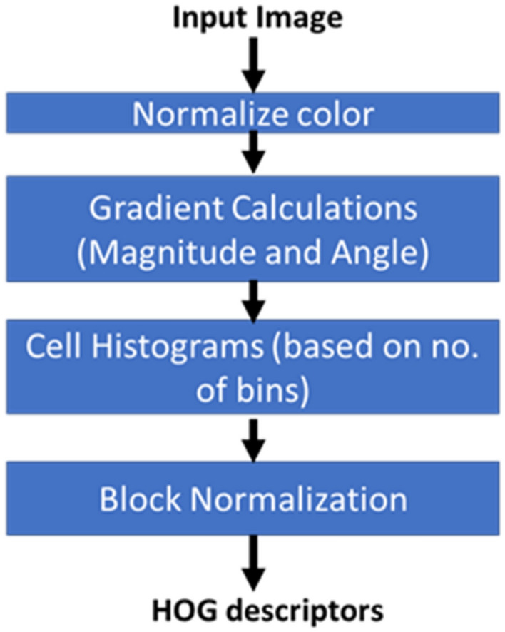
Histogram of oriented gradients (HOG) descriptor pipeline

After generating HOG descriptors for the slice set, the trained Support Vector Machine (SVM) classifier is used to differentiate the opened lung slices from the closed lung slices. Moreover, sample output slices are inspected and verified by a medical expert to ensure opened lung slices are correctly separated from closed ones.

Feature analysis and classification phase

Feature analysis and classification

Automatic segmentation of medical image is considered the most important process for RoI extraction (Hawas et al. 2019; Sengur et al. 2019). It divides images into areas based on a specified description, such as segmenting body tissues, border detection, tumor segmentation and mass detection (Hawas et al. 2019; Sengur et al. 2019). Most datasets do not have ground truth masks for lung parenchyma because creating masks requires intensive work from physicians. So, a common approach is to resort to unsupervised segmentation (Hasan et al. 2020; Wu et al. 2020).

Unsupervised clustering-based segmentation is proposed for lung parenchyma segmentation in COV-CAF to eliminate the need for exhaustive manual annotation. In this stage, automatic unsupervised segmentation is based on clustering approach. Fuzzy C-means (FCM) and K-means clustering algorithms are applied and the appropriate clustering approach is chosen based on the clustering validity measures, namely Davis-Bouldin index, Silhouette Index and Dunn Index. FCM algorithm (Kang et al. 2009) helps identify the boundaries of lung parenchyma from the surrounding thoracic tissue in 2D-CT axial view slices. Hence, FCM is more likely to be used in this stage because of its known accurate RoI segmentation of irregular and fuzzy borders compared to different other techniques as K-means (Kang et al. 2009; Wiharto and Suryani 2020). Therefore, the FCM algorithm is presented in Algorithm 1. The algorithm is based on the minimization of the objective function shown in Eq. (3) where D is the number of data points, N is the number of clusters, m is fuzzy partition matrix exponent for controlling the degree of fuzzy overlap, x_i is the ith datapoint, c_j is the center of the jth cluster and and μ_ij is the degree of membership of x_i (the sum of all membership values for all the clusters are 1) (Bezdek et al. 1984)

$$J_m=\sum _{i=1}^D\sum _{j=1}^N{\mu }_{\mathit{ij}}^m|\left|x_i-c_j\right|{\left(\right|}^2$$ 3

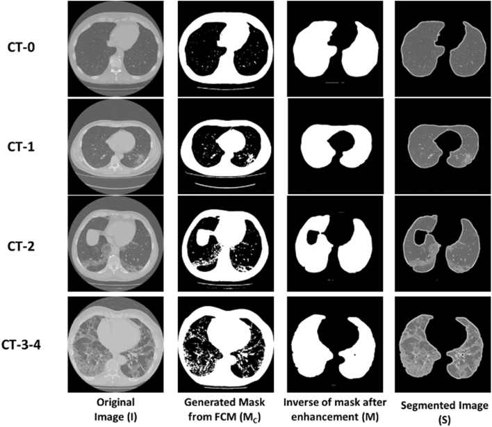
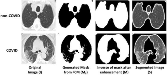
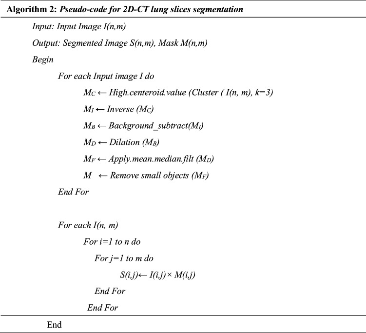
The whole segmentation process is described in Algorithm 2 which starts by selecting the best number of clusters (k) then image enhancement is applied. The best number of clusters is determined experimentally by applying a set of clustering quality measures which are Elbow method, Davis-Bouldin index, Silhouette Index and Dunn Index. Several number of clusters (k) are attempted and the number of cluster (k) with the best corresponding quality measures is selected for mask generation and segmentation. The used mask for Image (I) is the mask generated from the highest centroid value, which succeeds in identifying the boundaries of lung parenchyma correctly (M_C). Samples of the generated masks are shown in Figs. 5 and 6. After that, the centroid mask corresponding to each image is inversed producing M_I and background is subtracted to generate M_B image. The inversed mask with subtracted background (M_B) is preprocessed by a set of morphological operations filtered by different filtration masks giving intermediate images M_D and M_F respectively. Finally, the small, connected objects (due to deficiency of segmentation) are removed creating the final mask M. After generating the mask for all images in the dataset, the mask is multiplied by its corresponding image and the RoI is segmented. Samples of inverse mask after enhancement and segmented RoI is shown in Figs. 5 and 6.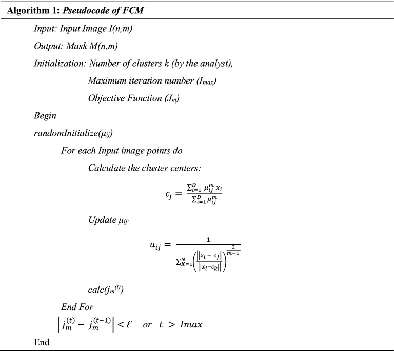

Fig. 5.

MosMedData: mask generation and RoI segmentation for different dataset samples for different classes

Fig. 6.

SARS-COV-2: mask generation and RoI segmentation for different dataset samples for different classes

Modified norm-VGG16 deep learning architecture

Over the years, Deep leaning architectures have progressed rapidly. The main advantage of deep learning architecture is automatic generation of features without any human intervention. However, one of the common concerns of deep learning architectures is the limited interpretability of the constructed models (Ibrahim et al. 2020) due to its black box nature which may lower the usability of the system by medical experts, who are keen on explainable decisions. One of the well-known deep learning architectures is the VGGs architectures. VGGs (Simonyan and Zisserman 2014) are known for their superior performance compared to different CNN architectures like AlexNet (Krizhevsky et al. 2017).

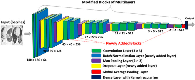
A modified version of VGG16 (Simonyan and Zisserman 2014) is proposed “Norm-VGG16” which is adopted from (Ibrahim et al. 2020) due to its accurate results compared to other architecture like ResNets, Inceptions and MobileNet architectures. Before training the Norm-VGG16, the RoI area of lung parenchyma in 2D-CT slice is cropped by applying a bounding box between X_initial to X_final pixels in the x-axis and Y_initial to Y_final pixels in the y-axis ([X_intial,Y_initial] to [X_final,Y_final]). The values of X_initial, X_final, Y_initial and Y_final are determined experimentally. The cropping of images is done to focus on the RoI in the images before passing it to the CNN and starting the training process. After image cropping, all images are normalized because images may have highly varying pixel range that could cause differences in the resultant loss (Ibrahim et al. 2020). The high pixel range will always have a large number of votes in updating weights of kernels in CNN layers in comparison with low pixel range. So, normalization of images decreases the gap and make a fair competition between high pixel ranges and low pixel ranges (Ibrahim et al. 2020). The structure of the Norm-VGG16 is modified to have an input of 180 × 180 followed by 16 convolution layers and each convolution layer is followed by batch normalization layer. Max pooling layers and dropout layers are added between convolution blocks and the CNN ends with global average pooling layer and categorical dense layer with kernel regularizer as shown in Fig. 7.

Fig. 7.

Modified NormVGG16 architecture

1. Convolution layers

   Its main role is automatic feature extraction by passing different number of kernels (feature maps) on the input image (Srinivas et al. 2016). The kernel weights change during the training stage and are settled at the end of the training stage to be used in the testing stage. In Norm-VGG16, the kernel size is 3 × 3 and stride = 1. The number of kernels (feature maps) is different in each convolution layer as shown in Fig. 7. The pipeline of CNN starts with a convolution layer with 64 feature maps (3 × 3 × 64) and the last convolution layer of the pipeline has 512 feature maps (3 × 3 × 512).

2. Sub-sampling (max pooling/global average pooling) layers

   Sub-sampling layers produce a down-sampled version that is robust against noise and distortion (Srinivas et al. 2016). Norm VGG16 uses different types of sub-sampling layers which are max pooling layers and average pooling layers. The max pooling layers consider the highest activation value of a window of size n × n of each feature map (Srinivas et al. 2016). Max pooling layers in NormVGG16 have [2 × 2] kernel size. The global average pooling layer computes the mean value of each feature map and forward it to the SoftMax in dense layer. The SoftMax in dense layer takes each value and converts it to a probability (with the probability of all digits summing to 1.0) (Mohsin and Alzubaidi 2020).

3. Batch normalization and dropout layers

   NormVGG16 is a deep CNN which is prone to overfitting of training data (Ioffe and Szegedy 2015; Srivastava et al. 2014). Batch Normalization layers and Dropout layers prevent overfitting of Deep CNNs. In Dropout layers, the term “dropout” refers to dropping out units (hidden visible) in a neural network. Dropping a unit out means it is temporarily removed from the network, along with all its incoming and outgoing connections (Srivastava et al. 2014). The choice of which units to drop is random. Each unit is retained with a fixed probability p independent of other units (Srivastava et al. 2014). Batch Normalization allows using higher learning rates and reduces the dependence on initialization. It also acts as a regularizer and helps dropout layers in avoiding overfitting (Ioffe and Szegedy 2015).

4. Kernel regulaizers

   Kernel regularizers (L2) is added to the dense layer in NormVGG16. Kernel regulaizers is used to decrease overfitting by increasing the loss equation during training phase by a factor as shown in Equation 4 where a training function ŷ: f(x) should be first defined as a function that maps an input vector x to output ŷ where ŷ is predicted value for actual value y. Loss (L) can be computed as L((y_i), ŷ_i) = L (f(x_i), y_i) (Chris 2020). For all input samples x_i … X_n. The sum of all loss functions between each input xi and its corresponding output ŷ. The factor of increasing loss is proportional to the square of the value of the weight coefficients.

   $$L\left(f\left(x_i\right),y_i\right)=\sum _{i=1}^n{L}_{\mathit{losscomponent}}\left(f\left(x_i\right),y_i\right)+\lambda \sum _{i=1}^n{w}_i^2$$ 4

Kernel regulaizers were first added in different layers but best performance was attained when it is added to the last layer (dense layer).

Over all, the proposed modifications in Norm-VGG16 can be summarized as increasing the number of convolution layers from 13 to 16 layers, addition of batch normalization layer after each convolution layer, addition of a dropout layer after each max pooling layer and integrating a kernel regularizer to the global average pooling layer. The additional added layers (batch normalization and dropout) and kernel regularizer plays an important role in opposing overfitting of the standard VGG16 network during training process.

Spatial feature extraction and fusion

The benefit of feature fusion is the detection of correlated feature values generated by different algorithms (Ross 2009). The fusion of features of different properties and families creates a compact set of salient features that can improve robustness and accuracy of classification model (Ross 2009). In this stage, spatial feature descriptors of global and local features are extracted from CT images and fused with the automatic features generated from modified NormVGG16.

After automatic segmentation of lung from CT slices, all the segmented images are resized to 64 × 64 to decrease as much as possible the size of extracted spatial features from the segmented RoI. Two articulated spatial features are extracted from the slices which are HOG and DAISY descriptors. The HOG feature descriptors were explained in detail in Sect. 3.1.2.

The DAISY descriptor is used because it is designed for effective dense computation as it is faster than GLOH and SIFT feature descriptors (Tola et al. 2010) and can be computed effectively unlike SURF (Tola et al. 2010). The DAISY feature descriptors generate low dimensional invariant descriptors from local image regions. Eight orientation maps, G, are generated for each direction and are computed for each image to generate its DAISY descriptors (Tola et al. 2010). Gaussian kernels of different summation values convolve each orientation map several times to obtain convolved orientation maps (Tola et al. 2010). If G(u,v) is the image gradient at location (u, v) and the h_∑(u, v) is the vector made of values at location (u,v) in the orientation maps after convolution by gaussian kernels then the standard deviation can be calculated as in Eq. (5) (Tola et al. 2010).

$$h_{\sum 1}\left(u,v\right)={\left[G_1^{\sum 1}\left(u,v\right),\dots ,G_H^{\sum 1}\left(u,v\right)\right]}^T$$ 5

where G₁^∑, G₂^∑…G_H^∑ denote the Σ-convolved orientation maps (Tola et al. 2010). After that a normalization process occurs for each histogram independently to correctly represent the pixels near occlusions. The DAISY descriptors are calculated for different layers of concentric circles as shown in Fig. 8. The full DAISY descriptors D (u₀, v₀) for location (u₀, v₀) is then defined as a concatenation of h vectors at different layers of concentric circles as shown in Eq. (6).

$$D\left(u_0,,,v_0\right)={\left[\begin{array}{c}{\widehat{h}}_{\sum 1}^T\left(u_0,,,v_0\right),\\ {\widehat{h}}_{\sum 1}^T\left(I_1,\left(u_0,,,v_0,,,R_1\right)\right),\cdots \cdots \cdots \cdots {\widehat{h}}_{\sum 1}^T\left(I_N,\left(u_0,,,v_0,,,R_1\right)\right),\\ {\widehat{h}}_{\sum 2}^T\left(I_1,\left(u_0,,,v_0,,,R_2\right)\right),\cdots \cdots \cdots \cdots {\widehat{h}}_{\sum 2}^T\left(I_N,\left(u_0,,,v_0,,,R_2\right)\right),\\ {\widehat{h}}_{\sum Q}^T\left(I_1,\left(u_0,,,v_0,,,R_3\right)\right),\cdots \cdots \cdots \cdots {\widehat{h}}_{\sum Q}^T\left(I_N,\left(u_0,,,v_0,,,R_3\right)\right),\end{array}\right]}^T$$ 6

where Q is the number of convolved orientation layers with different ∑’s and Ij (u, v, R) is the location with distance R from (u,v) in the direction given by j when the directions are quantized into N layers of concentric circles as shown in Fig. 8.

Fig. 8.

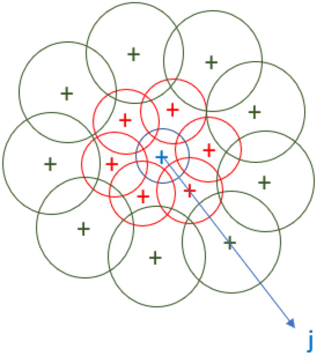
DAISY descriptors layers of concentric circles

HOG descriptors are from global features family that generates a compact texture features but they are most sensitive to clutter and occlusion (Lisin et al. 2005). On the other hand, DAISY descriptors are from local features family which generates key descriptors that are calculated in multiple interest points of local image and are not sensitive to clutter and occlusion (Lisin et al. 2005). The key point of extracting both, HOG and DAISY descriptors, is to combine different information of different families of features, which is expected to improve the results (Lisin et al. 2005).

After extracting spatial features, the 512 features, generated by the Norm-VGG16 from the global average pooling layer shown in Fig. 7, are fused with 8100 HOG descriptors generated for each segmented image and 400 DAISY descriptors. After fusion of automatic generated features and hand-crafted features, the fused 9012 features are used for classification.

Classification

After the spatial features and automatic features are extracted and fused, the CT-slices are classified using Linear Support Vector Machine (SVM) based on the merged features. SVM finds the suitable hyperplane that maximizes the margin between classes (Cortes and Vapnik 1995). The SVM classifier has been chosen due to its robustness because SVM is trained by solving a constrained quadratic optimization problem (Cortes and Vapnik 1995). This means that each SVM parameter has only a unique optimal solution, unlike other classifiers, such as standard Neural Networks which are trained using backpropagation (Cortes and Vapnik 1995). Due to the large size of fused features which is equal 9012 × n, where n is the number of CT slices in dataset, the full dataset is too large and can’t fit completely in RAM. Incremental learning (Diehl and Cauwenberghs 2003) is used, which means dividing the dataset into batches during training of SVM, batch by batch is loaded from Hard disk to RAM to overcome the limited RAM bandwidth.

Materials

In the current study, two benchmark datasets are used in experiments of the proposed models. The two datasets are MosMedData: Chest CT Scans with COVID-19 Related Findings dataset and SARS-COV-2 CT-Scan dataset.

MosMedData: chest CT scans with COVID-19 related findings dataset

The MosMedData dataset (Morozov et al. 2020) was provided by medical hospitals in Moscow, Russia and collected at Center of Diagnostics and Telemedicine. It comprises 1110 3D-CT (saved as NifTi format) lung volumes of anonymized human lung computed tomography (CT) scans with COVID-19 related findings, as well as without such findings. The dataset includes 42% males, 56% females and 2% others of ages between 18 and 97 years old with median of 47 years old. Each 3D-CT NifTi volume corresponds to unique patient. The dataset is characterized by the availability of labeled different severity levels. The levels indicate the impact of COVID-19 infection on lungs. Such characteristic shall aid the precise diagnosis of COVID-19 and identification of subjects of high risk that need immediate intervention.

The 3D CT-volumes are divided into 5 classes depending on the state of the lung tissue which are:

• CT-0: normal lung tissue, no CT-signs of viral pneumonia.

• CT-1: several ground-glass opacifications, involvement of lung parenchyma is less than 25%.

• CT-2: ground-glass opacifications, involvement of lung parenchyma is between 25 and 50%.

• CT-3: ground-glass opacifications and regions of consolidation, involvement of lung parenchyma is between 50 and 75%.

• CT-4: diffuse ground-glass opacifications and consolidation as well as reticular changes in lungs. Involvement of lung parenchyma exceeds 75%.

The distribution of volumes over the severity classes is shown in Table 1.

Table 1.

MosMedData: chest CT scans with COVID-19 related findings dataset distribution of 3D-CT volumes studies

CT-0	CT-1	CT-2	CT-3	CT-4	Total
254	684	125	45	2	1110
22.88%	61.62%	11.26%	4.05%	0.18%	100%

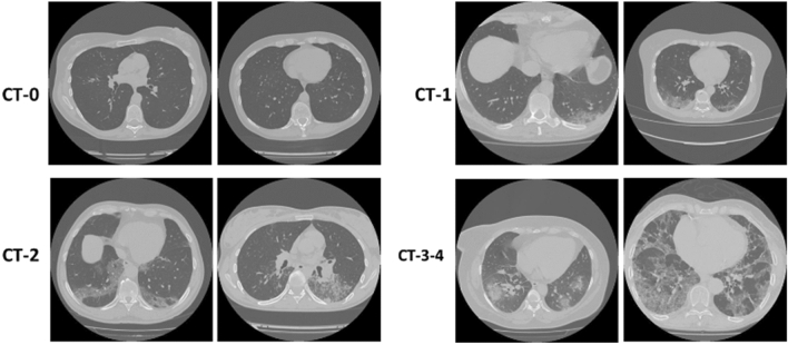
In accordance with clinical experts’ recommendation and due to the limited percentage of 3D subjects in CT-4, it is combined with the previous class CT-3 creating a composite class called (CT-3–4), which denotes the severe cases who have ground-glass opacifications and consolidation, involvement of lung parenchyma exceeding 50%. As of this modification the new distribution of COVID-19 related findings severity is shown in Table 2. The four classes CT-0, CT-1, CT-2 and CT-3–4 are shown in Fig. 9.

Table 2.

MosMedData: chest CT scans with COVID-19 related findings dataset distribution of 3D-CT volumes studies after combination of CT-3 and CT-4 classes

CT-0	CT-1	CT-2	CT-3–4	Total
254	684	125	47	1110
22.88%	61.62%	11.26%	4.23%	100%

Fig. 9.

Slices from 3D volumes of MosMedData dataset classes after merging classes CT-3 and CT-4 to CT-3–4

After applying the Preparatory phase modules in Sect. 3, the dataset is divided into 90% as training dataset and 10% as testing dataset. The distribution of the classes within the training dataset is illustrated in Table 3 while the distribution of testing dataset is illustrated in Table 4.

Table 3.

Training dataset class distribution

CT-0	CT-1	CT-2	CT-3–4	Total
5746	14,792	2611	967	24,116
23.83%	61.34%	10.83%	4.01%	100%

Table 4.

Testing dataset class distribution

CT-0	CT-1	CT-2	CT-3–4	Total
639	1,644	291	108	2682
23.83%	61.30%	10.85%	4.03%	100%

SARS-COV-2 CT-scan dataset

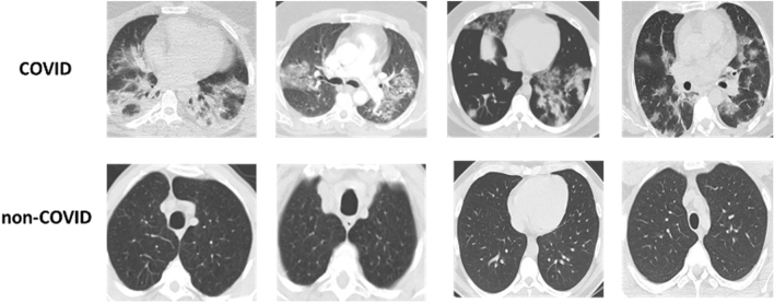
The SARS-COV-2 2D-CT-Scan dataset (Soares et al. 2020) consists of 2482 CT scan images. It is divided to 1252 CT scans that are positive for SARS-CoV-2 infection (COVID-19) and 1230 CT scans for normal subjects, non-infected by COVID-19. The dataset is collected from 120 real patients in hospitals of Sao Paulo, Brazil, of which 60 patients are infected by COVID-19 including 32 males and 28 females, and the other 60 patients are not infected by COVID-19, which are 30 males and 30 females. The used dataset is publicly available on www.kaggle.com/plameneduardo/sarscov2-ctscan-dataset. The dataset is divided into 90% as training dataset and 10% as testing dataset. The distribution of the classes within the training set is illustrated in Table 5 while the distribution of testing dataset is illustrated in Table 6. The two classes of the dataset can be shown in Fig. 10.

Table 5.

Training Dataset class distribution

Training dataset		Total
COVID	Non-COVID
1126	1106	2232
50.45%	49.55%	100%

Table 6.

Testing Dataset class distribution

Testing dataset		Total
COVID	Non-COVID
126	123	249
50.60%	49.40%	100%

Fig. 10.

Sample slices of SARS-COV-2 2D-CT-scan dataset (COVID and non-COVID)

Experimental results and discussion

Experimental environment: tools and setup

Automatic Segmentation is performed using MATLAB 2019a, while model implementation, training, and testing are done using Python language v3.7.6 with Keras package (TensorFlow backend). Experiments are conducted on core i7, 2.21 GHz processor with 16 GB RAM and Nvidia GTX 1050Ti with 4 GB RAM. All deep learning architectures are trained for 50 epochs from scratch using Adam optimizer with starting learning rate of 0.001. Inputs are divided into batches of size 32. Validation accuracy and cross-entropy loss are monitored for each epoch. In addition, the learning rate is reduced by factor of 0.2 for each three epochs without improvement in validation loss. The best model is defined as having minimum validation loss, then it is stored and applied on the testing set.

Performance metrics

A set of performance measures is used to evaluate the used unsupervised segmentation clustering techniques in terms of the segmentation partitions quality. In addition, various established metrics are used to contrast the performance of the proposed COV-CAF architecture to the state-of-the-art models.

Segmentation performance indicators

Different qualitative metrics are used to evaluate the compactness and the degree of cluster separation for different unsupervised clustering algorithm to find the best clustering technique to be used with the best cluster numbers (Kovács et al. 2006; Youssef et al. 2007). After conducting the comparative experiments, the elbow method is used to ensures the appropriate number of clusters to be used.

1. Davis-Bouldin Index

   The measure is used to measure the ratio of the sum of within-cluster scatter to between-cluster separation. For C = (C₁…C_k) be a clustering centroid for a group of data objects (D) (Kovács et al. 2006; Youssef et al. 2007). So, Davis-Bouldin (DB) can be given as Eq. (7).

   $$DB=\frac{1}{k}\sum _{i=1}^k{R}_i\text{where}{R}_i=\underset{j=1\dots n,i\ne j}{max}{R}_{\mathit{ij}}$$ 7

   where R_ij is the similarity index that measures within-to-between cluster distance ratio an in Eq. (8).

   $$R_{\mathit{ij}}=\frac{{\overline{d}}_i+{\overline{d}}_j}{d_{i,j}}$$ 8
   The scatter measure for the centroids c_i of the Clusters C_i can be given as in Eq. (9).

   $$d\left(C_i\right)=\frac{1}{\left|C_i\right|}\sum _{x\in C_i}\left|\left|x-c_i\right|\right|$$ 9

   where || c_i—c_j || presents the cluster-to-cluster distance between centroids (c) of different clusters. The best value of DB is the low value of R_ij which generated from low value which represents low scatter value with high distance between cluster value (Youssef et al. 2007).

2. Silhouette Index

   It measures the average similarity of the objects within cluster and their distance to other objects in the other cluster (Wang et al. 2017) as shown in Eq. (10).

   $$s\left(i\right)=\frac{b\left(i\right)-a\left(i\right)}{max\left(a\left(i\right),b\left(i\right)\right)}$$ 10

   where a(i) is used to represents the average distance (d) of point i with respect to all other points belonging to same cluster C_i (shown in Eq. 11) while b(i) represents the average distance (d) of point i with respect to all other points in the nearest cluster C_k (shown in Eq. 12) (Wang et al. 2017).

   $$a\left(i\right)=\frac{1}{\left|{\text{C}}_{\text{i}}\right|-1}\sum _{j\in C_i,i\ne j}d\left(i,j\right)$$ 11

   $$b\left(i\right)=\underset{k\ne i}{min}\frac{1}{\left|C_k\right|}\sum _{j\in C_k}d\left(i,j\right)$$ 12
   The calculation of index involves that we choose minimum of all the average distance of the point i with all the other points that don't belong to another cluster. So, the general formula of Silhouette for Data points from 1…N can be written as shown in Eq. 13.

   $$S=\frac{1}{\text{N}}\sum _{i=1}^N{s}_i$$ 13

   So, it is concluded that the highest the ratio the better the clustering.

3. Dunn Index

   It determines the minimal ratio between cluster diameter and inter cluster distance and is calculated for Cluster Set C = (c1…ck) as shown in Eq. (14).

   $$D=\underset{c,d\in C}{min}\left[\frac{d\left({\mu }_c,{\mu }_d\right)}{\underset{c\in C}{max}\left[diam\left(c\right)\right]}\right]$$ 14

   where diam (c) is of cluster c computed as the maximum inner cluster distance and d(μc,μd), which is the distance between the centroids of clusters c and d, is maximized. So, the compact and well separated dataset must be expected to have large distance between clusters and small diameter. It is concluded that the highest Dunn index value represents better clustering technique and best number of clusters.

4. Elbow method

   After computing the clustering quality and validity measure, the Elbow method is applied to determine the best number of centroids for lung segmentation (Thorndike 1953). Elbow method is used to ensures the best number of clusters centroids to be used (Nanjundan et al. 2019; Thorndike 1953).

   1. Compute clustering algorithm for different k values (1:10).
   2. For each k, calculate the total within-cluster sum of square (wss).
   3. Plot a wss curve by number of clusters k.
   4. The location of a bend (knee) in the plot is considered as an indicator for the suitable clusters’ number.

Classification performance indicators

1. Confusion matrix

   Confusion Matrix is a summarize table for visualizing and describing the performance of model in classifying a testing set of data as the shown in Figure 11. It is a summary of prediction results in a classification problem (Ibrahim et al. 2020). In confusion matrix, values of True Positive (TP), True Negative (TN), False Positive (FP) and False Negative (FN) are represented by assuming Ci one of the four classes in our dataset.

   • TP (C_i) = All the instance of C_i, that are classified as C_i.
   • TN (C_i) = All the non-C_i, instances that are not classified as C_i.
   • FP (C_i) = All the non-C_i, instances that are classified as C_i.
   • FN (C_i) = All the C_i instances that are not classified as C_i.

2. Accuracy (Acc)

   It is calculated by dividing the number of images that are correctly labeled by the total number of test images. Equation (15) explain class accuracy measurements.

   $$Accuracy=\frac{TP+TN}{TP+TN+FP+FN}$$ 15

3. Precision (Prec)

   It is a metric which quantifies the number of positive predictions correctly made (Brownlee). Equation 16 explains single class precision measurements.

   $$Precision=\frac{\mathit{TP}}{\left(TP+FP\right)}$$ 16

4. Sensitivity (Sens)

   It is a metric which quantifies the number of correct positive predictions that could have been made from all the positive predictions (Brownlee). Equation (17) explains single class sensitivity measurements.

   $$Sensitivity=\frac{\mathit{TP}}{\left(TP+FN\right)}$$ 17

5. F-measure

   F-Measure is a metric that provides a way to combine both precision and sensitivity in a single metric to captures both properties (Brownlee). Equation (18) explains single class F-measure.

   $$F-measure=\frac{\left(2\ast Precision\ast Sensitivity\right)}{\left(Precision+Sesitivity\right)}$$ 18

6. Specificity (Spec)

   It is a metric that quantifies the number of correct negative predictions made from all negative predictions that could have been made (Brownlee). Equation (19) explains single class Specificity.

   $$Specificity=\frac{\mathit{TN}}{\left(TN+Fp\right)}$$ 19

Fig. 11.

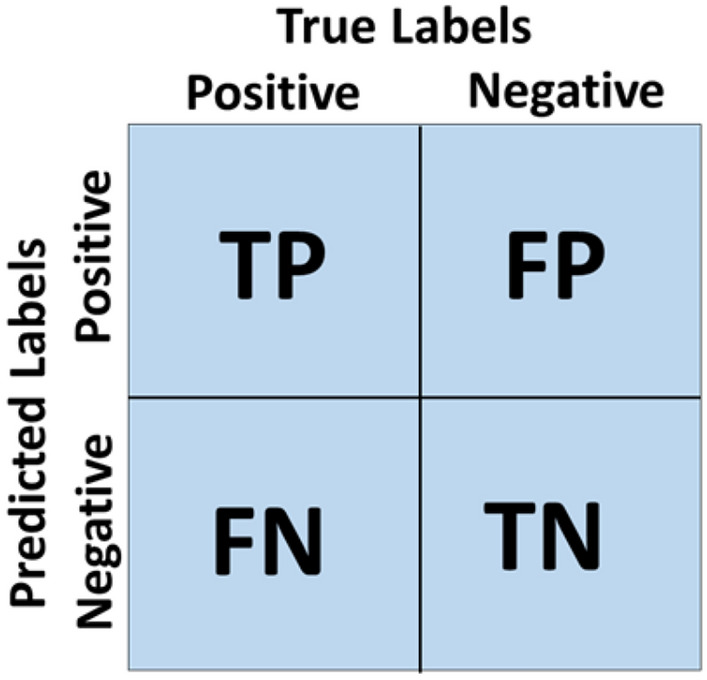
Confusion matrix

Experimental scenarios

In this section, the performance of the proposed COV-CAF system architecture and Norm-VGG16 is evaluated. Norm-VGG16 performance is reported as an independent pure DL classifier in the following experiments.

First, an ablation study is conducted on MosMedData: Chest CT Scans with COVID-19 Related Findings Dataset to emphasize the effect of each feature category and the fusion of features. Moreover, the effectiveness of the COV-CAF architecture, its backbone DL network (modified Norm-VGG16) and fused spatial articulated features on MosMedData: Chest CT Scans with COVID-19 Related Findings Dataset is illustrated against four prominent CNN architectures, namely Xception, ResNet-50, MobileNet-v2 and Inception-v3 applied on the entire CT image. In addition, the performance of COV-CAF is compared to traditional ML where SVM is applied on the extracted hand-crafted features only from the segmented ROI. COV-CAF performance is contrasted to pure DL and traditional ML approaches to elucidate the effect of fusing both methods. The four CNNs have a common modification of adding an input layer of size 180 × 180 and an output layer was modified to four neurons representing four classes of MosMedData: Chest CT Scans with COVID-19 Related Findings Dataset. The first experiment was conducted using Inception-v3 which is a model developed by google. It is a very deep network consists of 48 layers. It starts with 6 convolution layers and followed by 10 inception blocks. The full architecture is described in detail in (Szegedy et al. 2016). The Second experiment was conducted using MobileNet-v2 which is a light-weight network. It has 53 layers which are divide to 52 convolution layers and the last is the dense layer. The network start with 16 residuals and bottlenecks blocks and ends with one convolution layer followed by dense layer (Ardakani et al. 2020; Sandler et al. 2018). Third Experiment conducted by using ResNet-50 which is an architecture with 50 convolution layers. The architecture is based on residual blocks of two types of residual networks which are identity residual networks and shortcut residual networks (Soares et al. 2020). The full architecture is explained in (Ibrahim et al. 2020). The last experiment is done with the Xception network which has 71 layers. It started by two convolution layers followed by depth separable convolution layers, four convolution layers and dense layer (Ardakani et al. 2020). The full architecture and specification is explained in Chollet (2017). These four CNNs are chosen to implement and compare our proposed models because of their different depths, subsequent complexities and different theories of operations as was explained previously. Moreover, they are chosen because of their good results (Ardakani et al. 2020; Jaiswal et al. 2020).

Second, the effectiveness of the COV-CAF architecture and its backbone DL network (Norm-VGG16) is compared to Jaiswal et al. implemented deep learning models (Jaiswal et al. 2020) on SARS-COV-2 CT-Scan dataset.

Segmentation evaluation

Different number of experiments are applied on MosMedData: chest CT scans with COVID-19 Related Findings Dataset using different clustering indicators are applied to compare between different clustering techniques with varying number of clusters to determine the best algorithm to apply and best cluster number.

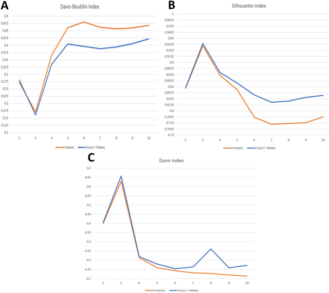
First, the comparisons between k-means and FCM clustering are shown in Table 7 and Fig. 12a, which depict that FCM always scores the lowest Davis-Bouldin values with different number of clusters (from 1 to 10 clusters) compared to k-means with the same number of clusters. Moreover, it was found that the best cluster number for FCM is (k) is three.

Table 7.

Davis-Bouldin index, Silhouette index and Dunn index for K-means and FCM for different number of clusters

No. of clusters (k)	Davis–Bouldin Index		Silhouette Index		Dunn Index
	K-means	FCM	K-means	FCM	K-means	FCM
2	0.27176	0.27997	0.84657	0.84839	0.39929	0.40432
3	0.17135	0.16057	0.93450	0.93920	0.62890	0.65713
4	0.36474	0.33448	0.87381	0.87908	0.21406	0.21948
5	0.46005	0.40427	0.84385	0.85726	0.16064	0.17965
6	0.47942	0.39610	0.78656	0.83318	0.14337	0.15385
7	0.46085	0.38838	0.77244	0.81777	0.13161	0.16337
8	0.45613	0.39438	0.77421	0.82022	0.12803	0.26181
9	0.45913	0.40567	0.77543	0.82778	0.12015	0.15875
10	0.46786	0.42155	0.78759	0.83192	0.11318	0.17251

Fig. 12.

Evaluation curves for different unsupervised clustering techniques. a Davis-Bouldin Index Curve. b Silhouette Index Curve. c Dunn Index Curve

Second, it was depicted from Silhouette index results in Table 7 and Fig. 12b that the FCM algorithm achieves the highest score compared to k-means with different number of clusters (from 1 to 10 clusters) which confirms that FCM is more suitable for our segmentation with cluster number (k) equals to three.

Finally, Table 7 and Fig. 12c provide certainty in choosing the FCM algorithm over the k-means as the highest Dunn index’s score achieved by FCM algorithm at number of clusters equals three that surpassed k-means with the same number of clusters.

Overall, the experimental findings stipulate on the superiority of FCM algorithm compared to k-means in unsupervised segmentation (Kang et al. 2009; Wiharto and Suryani 2020). In addition, the results in Table 7 show that the best number of clusters (k) equals three for both algorithms on MosMedData: Chest CT Scans with COVID-19 Related Findings Dataset.

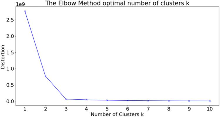
For more certainty for the best number of clusters centroids, the elbow method is used to ensure the perfect number of clusters suitable for our experiments and it was found that the bend in the curve is at cluster number (k) equals to three as shown in Fig. 13.

Fig. 13.

FCM Elbow method using wss curve for optimal number of clusters (K)

Classification results

MosMedData: chest CT scans with COVID-19 related findings dataset

A preliminary experiment is carried out to verify the candidacy of Norm-VGG16 as the backbone (feature extractor) of the COV-CAF architecture. The mean performance metrics of five different bootstrapped partitions using the described DL architectures are shown in Table 8. Bootstrapping is used to show the performance stability and robustness across a set of different partitions. Overall, Norm-VGG16 achieves the best mean performance metrics except for specificity. It attained an overall accuracy of 96.64% and macro average of precision, sensitivity, specificity and f-measure of 96.92, 93.65%, 97.2% and 95.26%, respectively. Hence, Norm-VGG16 is used as the feature extractor within the COV-CAF architecture.

Table 8.

The pure DL architectures mean performance of five different bootstrapped partitions experiment applied on the entire MosMedData: chest CT scans with COVID-19 related findings

Models	Mean overall acc (%)	Mean prec (%)	Mean sens (%)	Mean F-measure (%)	Mean spec (%)
The proposed modified Norm-VGG16	96.64	96.92	93.65	97.2	95.26
Xception	94.89	94.00	90.63	92.58	96.58
ResNet-50	92.80	92.50	88.00	90.03	94.98
MobileNet-v2	92.72	92.77	88.00	89.80	95.80
Inception-v3	90.58	86.89	85.23	85.98	95.63

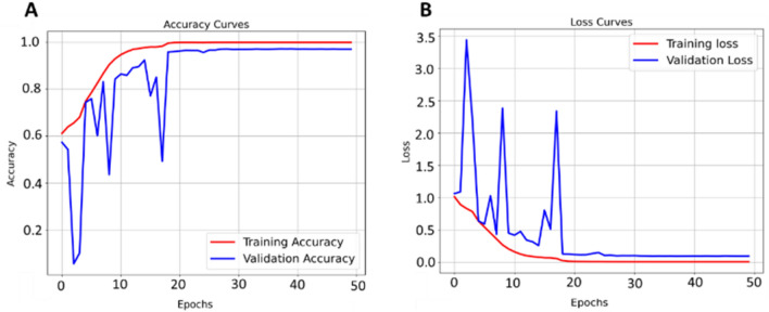
The Norm-VGG16 learning (training and testing) curves of the best model partition are shown in Figure 14. The best model achieves a training accuracy of 99.98% and testing accuracy of 97.09%. The learning curves manifest that the testing accuracies and losses are stabilized around the 25th epoch. The gap between the training and testing curves, either in accuracy curves or in loss curve, can be due to the small amount of testing set compared to training dataset, thus a gap in performance might exist. To compensate for such possibility, the bootstrapping experiment is conducted to provide a robust illustration of the accuracy of the model and to ensure that the proposed modified Norm-VGG16 is not overfitting on one partition of the bootstrapped experiments

Fig. 14.

Norm-VGG16 learning curves. a Training and testing accuracy curves. b Training and testing loss curves

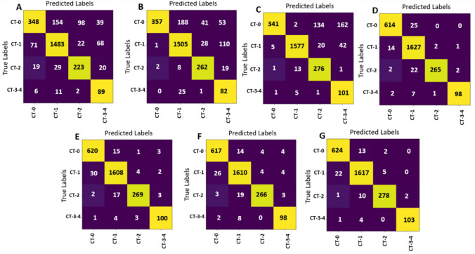
The remaining experiments are conducted using 90/10 percentage split. Tables 9 and 10 depict the calculated performance metrics of Norm-VGG16 applied directly on the entire CT image and COV-CAF architecture, respectively. The results of Norm-VGG16 model and COV-CAF are calculated from the best generated confusion matrices in Fig. 15f, g, respectively. In Tables 9 and 10, the accuracy, precision, sensitivity, f-measure and specificity are calculated for each class separately and a marco average for each performance metric is calculated. The macro average computes the performance metric independently for each class and then calculate their average. Tables 9 and 10 reveal that the hybrid model surpasses its counterpart Norm-VGG16 in terms of macro average metrics: accuracy, sensitivity and F-measure. with differences of 2.51%, 2.51% and 1.37% respectively.

Table 9.

The proposed modified Norm-VGG16 performance metrics calculated on MosMed dataset

Evaluation metric/class	Acc (%)	Prec (%)	Sens (%)	F-measure (%)	Spec (%)
CT-0	96.08	97.15	96.09	96.62	99.12
CT-1	98.97	96.79	98.97	97.87	94.80
CT-2	91.07	98.88	91.07	94.81	99.87
CT-3–4	90.74	97.03	90.74	93.78	99.88
Macro average	94.22	97.46	94.22	95.77	98.42

Table 10.

The proposed COV-CAF architecture performance metrics calculated on MosMed dataset

Evaluation metric/class	Acc (%)	Prec (%)	Sens (%)	F-measure (%)	Spec (%)
CT-0	97.65	96.30	97.65	96.97	98.83
CT-1	98.36	98.36	98.36	98.36	97.40
CT-2	95.53	97.54	95.53	96.52	99.71
CT-3–4	95.37	98.10	95.37	96.72	99.92
Macro average	96.73	97.58	96.73	97.14	98.97

Fig. 15.

Confusion Matrices of ablation models applied on MosMed dataset. a HOG + SVM model confusion matrix. b DAISY + SVM model confusion matrix. c Spatial articulated feature fusion (HOG + DAISY) + SVM confusion matrix. d The proposed modified Norm-VGG16 confusion matrix. e The proposed modified Norm-VGG16 + HOG confusion matrix. f The proposed modified Norm-VGG16 + DAISY confusion matrix. g The proposed COV-CAF Model confusion matrix

The performance of the proposed COV-CAF model and the effect of each feature of extracted features (HOG, DAISY and automatic features of proposed modified Norm-VGG16) and their different combinations are illustrated through an ablation study, where several combinations are experimented and contrasted. The confusion matrices for different extracted features and fusions are shown in Fig. 15 which is used in establishing Table 11 for accuracies comparison. From Table 11, it can be seen that fusion of the extracted spatial articulated features (HOG + DAISY) results in a significant increase in detecting the severe COVID-19 classes by scoring 85.57% which exceeds the accuracies of HOG extracted features and DAISY extracted features by 5.67% and 3.32% respectively. Comparing the accuracies of the fused spatial articulated features (HOG + DAISY) to the accuracies produced by HOG features, a difference of 18.22% and 11.11% is found in CT-2 and CT-3–4 severe classes accuracies respectively. Also, the fused spatial articulated features scores higher accuracies compared to DAISY extracted features in CT-2 and CT-3–4 severe classes with a difference of 4.82% and 17.59% respectively. The proposed modified Norm-VGG16 surpasses the spatial articulated feature fusion with an increase in CT-0 and CT-1 classes by about 40% and 3.05% respectively, while the spatial articulated features fusion produces an increase in the CT-2 and CT-3–4 severe infections by 3.78% and 2.78% respectively. In terms of the proposed COV-CAF model, it achieves the highest accuracies in COVID-19 most severe classes that need immediate medical interpretation which are CT-2 and CT-3–4 scoring 95.53% and 95.37% respectively as shown in Table 11. Only the proposed modified Norm-VGG16 achieves a slight increase in cases of non-severe infection CT-1 class.

Table 11.

Comparison between accuracies per class and over all accuracy for each proposed model applied on MosMed dataset for ablation study

Accuracy/class model	CT-0 (%)	CT-1 (%)	CT-2 (%)	CT-3–4 (%)	Overall (%)
HOG + SVM	54.46	90.21	76.63	82.41	79.90
DAISY + SVM	55.87	91.55	90.03	75.93	82.25
Spatial articulated feature (HOG + DAISY) fusion  + SVM	53.36	95.92	94.85	93.52	85.57
The proposed modified Norm-VGG16	96.08	98.97	91.07	90.74	97.09
The proposed modified Norm-VGG16 + HOG + SVM	97.03	97.81	92.44	92.59	96.83
The proposed modified Norm-VGG16 + DAISY + SVM	96.55	97.93	91.41	90.74	96.01
The proposed COV-CAF model	97.65	98.36	95.53	95.37	97.76

The spatial articulated features (HOG + DAISY) fusion model, COV-CAF model and its back bone the proposed modified Norm-VGG16 model are compared with different deep learning architecture with different subsequent complexity which are Xception, Resnet-50, MobileNet-v2 and Inception-v3 models. The best confusion matrix for each model of the deep learning models on MosMed dataset is reported in Fig. 16a–d. The confusion matrices in Fig. 16 are used to calculate the performance metrics for each model. The best Xception model achieves a testing accuracy of 94.67%, the best ResNet-50 model achieves a testing accuracy of 93.33%, the best MobileNet-v2 model achieves a testing accuracy of 93.14% and the best Inception-v3 model achieves a testing accuracy of 91.13%.

Fig. 16.

Confusion matrices of different CNN models applied on MosMed dataset. a Xception model confusion matrix. b ResNet-50 model confusion matrix. c MobileNet-v2 model confusion matrix. d Inception-v3 model confusion matrix

Table 12 depicts accuracy per class and overall accuracy of each of the seven implemented models. It can be noticed that COV-CAF and Norm-VGG16 outperform the other models. Norm-VGG16 surpasses the best per-class and overall accuracies of the four recognized architectures with the smallest differences being 3.28%, 1.59%, 3.44%, 0.93% and 2.42% for classes CT-0, CT-1, CT-2, CT-3–4 and overall accuracy, respectively. Despite that traditional ML of spatial articulated feature (HOG + DAISY) fusion scores the worst CT-0 accuracy across all models, it surpasses the standard DL architectures in terms of the critical classes (high severity) accuracy which are classes CT-2 and CT 3–4. A possible explanation for the variation in performance of the spatial articulated features (HOG + DAISY) is that the lack of evident textural changes in the soft tissues of CT-0 and CT-1 cases hinders the extraction of informative features for these classes. However, the high concentration of GGOs in the high severity classes (CT-2 and CT-3–4) generates large number of key features that are captured easily by HOG and DAISY features which are representatives of local and global features families respectively (Ahmed et al. 2017; Walsh et al. 2019). When compared to the proposed modified Norm-VGG16 deep learning architecture, it is found that traditional learning (HOG + DAISY) fusion model needs a smaller training dataset. Thus, spatial articulated feature (HOG + DAISY) fusion produces better accuracy results from the limited training set of the high severity cases (CT-2 and CT-3–4) (Walsh et al. 2019). This finding explains the superior performance of COV-CAF model, as it combines both features’ categories (automatic deep learning features + spatial articulated features) resulting in better overall performance. The proposed COV-CAF model attains the highest per-class accuracies except for CT-1 with a minute difference of 0.61% scored by Norm-VGG16. A remarkable improvement is reached by COV-CAF architecture compared to the four standard DL architectures, especially in the highest severity classes of CT-2 and CT-3–4. The improvements in CT-2 range from 10.31 to 14.77%, while a bigger range exist for CT-3–4 from 5.56 to 15.74%. The results elucidate the capability of COV-CAF architecture in stratifying the critical minority cases in contrast to the pure DL architectures. It also reveals a huge improvement over traditional ML in terms of CT-0 accuracy with 44.29% increase.

Table 12.

Comparison between accuracies per class and over all accuracy of different models applied on MosMed dataset

Accuracy/class model	CT-0 (%)	CT-1 (%)	CT-2 (%)	CT-3–4 (%)	Overall (%)
Spatial articulated feature (HOG + DAISY) fusion  + SVM	53.36	95.92	94.85	93.52	85.57
Inception-v3	87.79	95.01	80.76	79.63	91.13
MobileNet-v2	89.51	96.53	85.22	84.26	93.14
ResNet-50	89.51	96.53	87.63	82.41	93.33
Xception	92.80	97.38	85.22	89.81	94.67
The proposed modified Norm-VGG16	96.08	98.97	91.07	90.74	97.09
The proposed COV-CAF model	97.65	98.36	95.53	95.37	97.76

Table 13 shows a comparison between the COV-CAF architecture, the modified Norm-VGG16, The spatial articulated features (HOG + DAISY) fusion model and the implemented standard DL architectures. Similar findings to Table 12 show at Table 13, where it depicts the great improvement of the COV-CAF architecture relative to the rest of models, where COV-CAF achieves the highest precision, sensitivity, f-measure and specificity. It surpasses Norm-VGG16 in macro average sensitivity and F-measure by 2.51% and 1.37% respectively. The modified Norm-VGG16, which comes second after COV-CAF, exceeded the results achieved by Xception in terms of precision, sensitivity, f-measure and specificity by 3.04%, 2.92%, 2.99% and 1.12% respectively. Moreover, it is noteworthy that modified NormVGG16 architecture succeeded in attaining such significantly higher performance metrics, while maintaining much lower network depth and subsequent complexity compared to Xception architecture.

Table 13.

Comparison between macro average precision, sensitivity, f-measure and specificity for different models applied on MosMed dataset

Models	Macro average
	Prec (%)	Sens (%)	F-measure (%)	Spec (%)
Spatial articulated feature (HOG + DAISY) fusion + SVM	73.45	84.41	72.92	95.82
Inception-v3	87.18	85.80	86.45	95.89
Mobilenet-v2	93.17	88.88	90.90	96.48
ResNet-50	92.80	89.02	90.80	96.54
Xception	94.42	91.30	92.78	97.30
The proposed modified Norm-VGG16	97.46	94.22	95.77	98.42
The proposed COV-CAF model	97.58	96.73	97.14	98.97

SARS-COV-2 CT-scan dataset

The performance of COV-CAF architecture and the proposed modified Norm-VGG16 on SARS-COV-2 CT-Scan Dataset is compared to the results of the state-of -art of Jaiswal et al. (2020), who reported satisfactory results on the dataset. Table 14 shows the comparison between Jaiswal et al. (2020) implemented models and our models. The results show that the modified Norm-VGG16 model matched the results of the best model in the work of Jaiswal et al. (2020), DenseNet 201, with much lower network depth and subsequent complexity. Modified Norm-VGG16 consists of only 16 convolution layers, contrasted to the 201 convolution layers of Jaiswal et al. (2020) DenseNet201. Moreover, results show that COV-CAF got a considerable increase in sensitivity, F-measure, specificity than DesnseNet201 (Jaiswal et al. 2020) by 2.12%, 1.3%, 1.61% and 1.34% respectively. The highest improvement is attained in sensitivity of COVID19 group, which is a crucial measure in assessing the performance of the model to be able to correctly identify subjects that need immediate medical attention.

Table 14.

Comparison between proposed models and state-of-the art models on SARS-COV-2 Ct-scan dataset

Model	Acc (%)	Prec (%)	Sens (%)	F-measure (%)	Spec (%)
VGG16 (Jaiswal et al. 2020)	95.45	95.74	95.23	95.49	95.67
Inception ResNet (Jaiswal et al. 2020)	90.90	90.15	92.06	91.09	89.72
ResNet-152V2 (Jaiswal et al. 2020)	94.91	92.92	97.35	95.09	92.43
DenseNet201 (Jaiswal et al. 2020)	96.25	96.29	96.29	96.29	96.21
The proposed modified Norm-VGG16	96.39	96.80	96.03	96.41	96.21
The proposed COV-CAF	97.59	96.88	98.41	97.63	97.82

Conclusion

In this paper, a novel hybrid computer aided diagnostic system COV-CAF is introduced. COV-CAF introduces a preparatory phase and feature extraction and classification phase. The preparatory phase starts with a preprocessing module for converting the 3D volumes to 2D slices followed by an effective slice selection module to select CT slices with COVID-19 symptoms. Automatic DL feature extraction is performed by a modified Norm-VGG16 CNN. An unsupervised fuzzy c-means clustering is used to segment the RoI (lung parenchyma). Moreover, a feature fusion module is introduced where automatic features generated by Norm-VGG16 is combined with spatial articulated features generated from RoI segmentation. The remarkable result achieved by the proposed COV-CAF model in detecting COVID-19 infection and classifying the severity degree of infection from chest CT slices proves the robustness of the model and the importance of feature fusion phase. Our modified Norm-VGG16 and hybrid model surpassed traditional ML and the four well-known tested pure deep learning architecture named Xception, ResNet-50, MobileNet-v2 and Inception-v3 on MosMedData dataset. Moreover, our COV-CAF surpassed Jaiswal et al. who implemented four deep learning models on SARS-COV-2 Ct-Scan dataset.

As for the future work, different unsupervised techniques can be tested on different datasets to have a full study on the best unsupervised segmentation technique with the best number of clusters. Moreover, experimenting with different articulated features to be fused to the system to test its effect on the model performance.

Overall, the proposed COV-CAF diagnostic framework is a robust framework that can aid physicians in stratifying subjects into different risk groups according to their COVID-19 CT findings. Moreover, COV-CAF is a reusable framework that is expected to achieve competitive results on similar problems. It provides effective solutions to different common issues involved in CT lung diagnosis, such as slice selection, RoI segmentation and multi-view feature analysis.

Availability of data and material

MosMedData: Chest CT Scans with COVID-19 Related Findings Dataset is available via https://mosmed.ai/en/ and SARS-COV-2 CT-Scan Dataset is available via www.kaggle.com/plameneduardo/sarscov2-ctscan-dataset.

Author contributions

Conceptualization, MRI, SMY and KMF; methodology, MRI, SMY and KMF; software, MRI; validation, MRI, SMY and KMF; formal analysis, MRI; investigation, MRI; resources, MRI and KMF; writing—original draft preparation, MRI; writing—review and editing, SMY and KMF; visualization, MRI; supervision, SMY and KMF; project administration, SMY and KMF All authors have read and agreed to the published version of the manuscript.

Funding

This research received no external funding.

Compliance with ethical standards

Conflict of interest

The authors declare no conflict of interest.

Ethics approval

Not Applicable Data are obtained from publicly available datasets https://mosmed.ai/en/ & www.kaggle.com/plameneduardo/sarscov2-ctscan-dataset.

References

- Ahmed KT, Irtaza A, Iqbal MA. Fusion of local and global features for effective image extraction. Appl Intell. 2017;47:526–543. doi: 10.1007/s10489-017-0916-1. [DOI] [Google Scholar]
- Alafif T, Tehame AM, Bajaba S, Barnawi A, Zia S. Machine and deep learning towards COVID-19 diagnosis and treatment: survey, challenges, and future directions. Int J Environ Res Public Health. 2021 doi: 10.3390/ijerph18031117. [DOI] [PMC free article] [PubMed] [Google Scholar]
- Ardakani AA, Kanafi AR, Acharya UR, Khadem N, Mohammadi A. Application of deep learning technique to manage COVID-19 in routine clinical practice using CT images: results of 10 convolutional neural networks. Comput Biol Med. 2020;121:103795. doi: 10.1016/j.compbiomed.2020.103795. [DOI] [PMC free article] [PubMed] [Google Scholar]
- Bai HX, et al. Artificial intelligence augmentation of radiologist performance in distinguishing COVID-19 from pneumonia of other origin at chest CT. Radiology. 2020;296:E156–E165. doi: 10.1148/radiol.2020201491. [DOI] [PMC free article] [PubMed] [Google Scholar]
- Bezdek JC, Ehrlich R, Full W. FCM: the fuzzy c-means clustering algorithm. Comput Geosci. 1984;10:191–203. doi: 10.1016/0098-3004(84)90020-7. [DOI] [Google Scholar]
- Brownlee J (2020) How to calculate precision, recall, and F-measure for imbalanced classification. https://machinelearningmastery.com/precision-recall-and-f-measure-for-imbalanced-classification/. Accessed 27 Nov 2020
- Chen H, Ai L, Lu H, Li H. Clinical and imaging features of COVID-19. Radiol Infect Dis. 2020;7:43–50. doi: 10.1016/j.jrid.2020.04.003. [DOI] [PMC free article] [PubMed] [Google Scholar]
- Chollet F (2017) Xception: deep learning with depthwise separable convolutions. In: IEEE conference on computer vision and pattern recognition, pp 1800–1807
- Chris (2020) What are L1, L2 and elastic net regularization in neural networks? https://www.machinecurve.com/index.php/2020/01/21/what-are-l1-l2-and-elastic-net-regularization-in-neural-networks/. Accessed 15 November, 2020
- Chung M, et al. CT imaging features of 2019 novel coronavirus (2019-nCoV) Radiology. 2020;295:202–207. doi: 10.1148/radiol.2020200230. [DOI] [PMC free article] [PubMed] [Google Scholar]
- Cortes C, Vapnik V. Support-vector networks. Mach Learn. 1995;20:273–297. doi: 10.1007/BF00994018. [DOI] [Google Scholar]
- Dalal N, Triggs B (2005) Histograms of oriented gradients for human detection. In: 2005 IEEE computer society conference on computer vision and pattern recognition (CVPR'05), 20–25 June 2005, pp 886–893, vol 881. 10.1109/CVPR.2005.177
- Diehl C, Cauwenberghs G. SVM incremental learning. Adapt Optim. 2003 doi: 10.1109/IJCNN.2003.1223991. [DOI] [Google Scholar]
- Doi K. Computer-aided diagnosis in medical imaging: historical review, current status and future potential. Comput Med Imaging Graph. 2007;31:198–211. doi: 10.1016/j.compmedimag.2007.02.002. [DOI] [PMC free article] [PubMed] [Google Scholar]
- Fan L, et al. Progress and prospect on imaging diagnosis of COVID-19. Chin J Acad Radiol. 2020;3:4–13. doi: 10.1007/s42058-020-00031-5. [DOI] [PMC free article] [PubMed] [Google Scholar]
- Gozes O et al (2020) Rapid AI development cycle for the coronavirus (COVID-19) pandemic: initial results for automated detection and patient monitoring using deep learning CT image analysis. abs/2003.05037
- Hamadi A, Yagoub DE (2018) ImageCLEF 2018: semantic descriptors for tuberculosis CT image classification. In: CLEF, 2018
- Hani C, Trieu NH, Saab I, Dangeard S, Bennani S, Chassagnon G, Revel MP. COVID-19 pneumonia: a review of typical CT findings and differential diagnosis. Diagnos Intervent Imaging. 2020;101:263–268. doi: 10.1016/j.diii.2020.03.014. [DOI] [PMC free article] [PubMed] [Google Scholar]
- Hasan A, Al-Jawad M, Jalab H, Shaiba H, Ibrahim R, Shamasneh A. Classification of Covid-19 coronavirus, pneumonia and healthy lungs in CT scans using Q-deformed entropy and deep learning features. Entropy. 2020;22:517. doi: 10.3390/e22050517. [DOI] [PMC free article] [PubMed] [Google Scholar]
- Hawas AR, Ashour AS, Guo Y (2019) Neutrosophic set in medical image clustering. In: Guo Y, Ashour AS (eds) Neutrosophic set in medical image analysis. Academic Press, pp 167–187. 10.1016/B978-0-12-818148-5.00008-4
- Ibrahim M, Fathalla K, Youssef S. HyCAD-OCT: a hybrid computer-aided diagnosis of retinopathy by optical coherence tomography integrating machine learning and feature maps localization. Appl Sci. 2020;10:4716. doi: 10.3390/app10144716. [DOI] [Google Scholar]
- Ioffe S, Szegedy C (2015) Batch normalization: accelerating deep network training by reducing internal covariate shift
- Jaiswal A, Gianchandani N, Singh D, Kumar V, Kaur M (2020) Classification of the COVID-19 infected patients using DenseNet201 based deep transfer learning Journal of Biomolecular Structure and Dynamics:1–8 doi:10.1080/07391102.2020.1788642 [DOI] [PubMed]
- Kamalov F, Cherukuri A, Sulieman H, Thabtah F, Hossain MA (2021) Machine learning applications for COVID-19: a state-of-the-art review
- Kang H, et al. Diagnosis of coronavirus disease 2019 (COVID-19) with structured latent multi-view representation learning. IEEE Trans Med Imaging. 2020;39:2606–2614. doi: 10.1109/TMI.2020.2992546. [DOI] [PubMed] [Google Scholar]
- Kang J, Min L, Luan Q, Li X, Liu J. Novel modified fuzzy c-means algorithm with applications. Digital Signal Process. 2009;19:309–319. doi: 10.1016/j.dsp.2007.11.005. [DOI] [Google Scholar]
- Koo HJ, Lim S, Choe J, Choi S-H, Sung H, Do K-H. Radiographic and CT features of viral pneumonia. Radiographics. 2018;38:719–739. doi: 10.1148/rg.2018170048. [DOI] [PubMed] [Google Scholar]
- Kovács F, Legány C, Babos A (2006) Cluster validity measurement techniques. In: Proceedings of the 5th WSEAS international conference on artificial intelligence, knowledge engineering and data bases
- Krizhevsky A, Sutskever I, Hinton GE. ImageNet classification with deep convolutional neural networks. Commun ACM. 2017;60:84–90. doi: 10.1145/3065386. [DOI] [Google Scholar]
- Li L, et al. Using artificial intelligence to detect COVID-19 and community-acquired pneumonia based on pulmonary CT: evaluation of the diagnostic accuracy. Radiology. 2020;296:E65–E71. doi: 10.1148/radiol.2020200905. [DOI] [PMC free article] [PubMed] [Google Scholar]
- Lisin DA, Mattar MA, Blaschko MB, Learned-Miller EG, Benfield MC (2005) Combining local and global image features for object class recognition. In: 2005 IEEE computer society conference on computer vision and pattern recognition (CVPR'05)-Workshops, 21–23 Sept., pp 47–47. 10.1109/CVPR.2005.433
- Lodwick GS. Computer-aided diagnosis in radiology: a research plan. Investig Radiol. 1966;1:72–80. doi: 10.1097/00004424-196601000-00032. [DOI] [PubMed] [Google Scholar]
- Long C, et al. Diagnosis of the Coronavirus disease (COVID-19): rRT-PCR or CT? Eur J Radiol. 2020;126:108961–108961. doi: 10.1016/j.ejrad.2020.108961. [DOI] [PMC free article] [PubMed] [Google Scholar]
- Mohsin Z, Alzubaidi L (2020) Convolutional neural network with global average pooling for image classification
- Morozov S et al. (2020) MosMedData: chest CT scans with COVID-19 related findings dataset. 10.1101/2020.05.20.20100362
- Nanjundan S, Sankaran S, Arjun C, Anand G (2019) Identifying the number of clusters for K-Means: a hypersphere density based approach
- Radiopaedia COVID-19 pneumonia. https://radiopaedia.org/cases/covid-19-pneumonia-45. Accessed November 25, 2020
- Rahimzadeh M, Attar A, Sakhaei SM (2020) A fully automated deep learning-based network for detecting COVID-19 from a new and large lung CT scan dataset. medRxiv:2020.2006.2008.20121541. 10.1101/2020.06.08.20121541 [DOI] [PMC free article] [PubMed]
- Ronneberger O, Fischer P, Brox T (2015) U-Net: convolutional networks for biomedical image segmentation. In: Navab N, Hornegger J, Wells WM, Frangi AF (eds) Medical image computing and computer-assisted intervention: MICCAI 2015. Springer International Publishing, Cham, pp 234–241
- Rony Kampalath M (2020) Chest X-ray and CT Scan for COVID-19. https://www.verywellhealth.com/medical-imaging-of-covid-19-4801178#citation-1. Accessed 20 Nov 2020
- Ross A (2009) Fusion, Feature-Level. In: Li SZ, Jain A (eds) Encyclopedia of Biometrics. Springer US, Boston, MA, pp 597–602. doi:10.1007/978-0-387-73003-5_157
- Sandler M, Howard A, Zhu M, Zhmoginov A, Chen L-CJICCoCV, Recognition P (2018) MobileNetV2: inverted residuals and linear bottlenecks, pp 4510–4520
- Sengur A, Budak U, Akbulut Y, Karabatak M, Tanyildizi E (2019) A survey on neutrosophic medical image segmentation. In: Guo Y, Ashour AS (eds) Neutrosophic set in medical image analysis. Academic Press, pp 145–165. 10.1016/B978-0-12-818148-5.00007-2
- Simonyan K, Zisserman A (2014) Very deep convolutional networks for large-scale image recognition. arXiv 14091556
- Singh D, Kumar V, Vaishali KM. Classification of COVID-19 patients from chest CT images using multi-objective differential evolution-based convolutional neural networks. Eur J Clin Microbiol Infect Dis. 2020;39:1379–1389. doi: 10.1007/s10096-020-03901-z. [DOI] [PMC free article] [PubMed] [Google Scholar]
- Soares E, Angelov P, Biaso S, Higa Froes M, Kanda Abe D (2020) SARS-CoV-2 CT-scan dataset: a large dataset of real patients CT scans for SARS-CoV-2 identification. medRxiv:2020.2004.2024.20078584. doi:10.1101/2020.04.24.20078584
- Srinivas M, Roy D, Mohan CK (2016) Discriminative feature extraction from X-ray images using deep convolutional neural networks. In: 2016 IEEE international conference on acoustics, speech and signal processing (ICASSP), 20–25 March 2016, pp 917–921. doi:10.1109/ICASSP.2016.7471809
- Srivastava N, Hinton G, Krizhevsky A, Sutskever I, Salakhutdinov R. Dropout: a simple way to prevent neural networks from overfitting. J Mach Learn Res. 2014;15:1929–1958. [Google Scholar]
- Szegedy C, Vanhoucke V, Ioffe S, Shlens J, Wojna ZJ, Recognition P (2016) Rethinking the inception architecture for computer vision 1:2818–2826
- Thorndike RL. Who belongs in the family? Psychometrika. 1953;18:267–276. doi: 10.1007/BF02289263. [DOI] [Google Scholar]
- Tola E, Lepetit V, Fua P. DAISY: an efficient dense descriptor applied to wide-baseline stereo. IEEE Trans Pattern Anal Mach Intell. 2010;32:815–830. doi: 10.1109/TPAMI.2009.77. [DOI] [PubMed] [Google Scholar]
- Walsh J, et al. Deep learning vs. Traditional Computer Vision. 2019 doi: 10.1007/978-3-030-17795-9_10. [DOI] [Google Scholar]
- Wang F, Franco-Penya H-H, Kelleher J, Pugh J, Ross R. An analysis of the application of simplified Silhouette to the evaluation of k-means. Cluster Validity. 2017 doi: 10.1007/978-3-319-62416-7_21. [DOI] [Google Scholar]
- Wang S-H, Nayak DR, Guttery DS, Zhang X, Zhang Y-D. COVID-19 classification by CCSHNet with deep fusion using transfer learning and discriminant correlation analysis. Inf Fusion. 2021;68:131–148. doi: 10.1016/j.inffus.2020.11.005. [DOI] [PMC free article] [PubMed] [Google Scholar]
- Wang S, et al. A fully automatic deep learning system for COVID-19 diagnostic and prognostic analysis. Eur Respir J. 2020;1:2000775. doi: 10.1183/13993003.00775-2020. [DOI] [PMC free article] [PubMed] [Google Scholar]
- Wiharto W, Suryani E. The comparison of clustering algorithms K-means and fuzzy C-means for segmentation retinal blood vessels. Acta Inform Med. 2020;28:42–47. doi: 10.5455/aim.2020.28.42-47. [DOI] [PMC free article] [PubMed] [Google Scholar]
- WorldOmeter COVID-19 coronavirus pandemic. https://www.worldometers.info/coronavirus/.
- Wu X, et al. Deep learning-based multi-view fusion model for screening 2019 novel coronavirus pneumonia: a multicentre study. Eur J Radiol. 2020;128:109041. doi: 10.1016/j.ejrad.2020.109041. [DOI] [PMC free article] [PubMed] [Google Scholar]
- Youssef S, Rizk M, El-Sherif M. Dynamically adaptive data clustering using intelligent swarm-like agents. Math Comput Simul. 2007;1:1. [Google Scholar]
- Zhang YD, Satapathy SC, Zhu LY, Górriz JM, Wang SH. A seven-layer convolutional neural network for chest CT based COVID-19 diagnosis using stochastic pooling. IEEE Sens J. 2020;1:1–1. doi: 10.1109/JSEN.2020.3025855. [DOI] [PMC free article] [PubMed] [Google Scholar]
- Zheng C et al (2020) Deep learning-based detection for COVID-19 from chest CT using weak label. medRxiv:2020.2003.2012.20027185. doi:10.1101/2020.03.12.20027185
- Zu ZY, Jiang MD, Xu PP, Chen W, Ni QQ, Lu GM, Zhang LJ. Coronavirus disease 2019 (COVID-19): a perspective from China. Radiology. 2020;296:E15–E25. doi: 10.1148/radiol.2020200490. [DOI] [PMC free article] [PubMed] [Google Scholar]
Associated Data
This section collects any data citations, data availability statements, or supplementary materials included in this article.
Data Availability Statement