Trans-ancestry genome-wide association meta-analysis of prostate cancer identifies new susceptibility loci and informs genetic risk prediction

Abstract

Prostate cancer is a highly heritable disease with large disparities in incidence rates across ancestry populations. We conducted a multiancestry meta-analysis of prostate cancer genome-wide association studies (107,247 cases and 127,006 controls) and identified 86 new genetic risk variants independently associated with prostate cancer risk, bringing the total to 269 known risk variants. The top genetic risk score (GRS) decile was associated with odds ratios that ranged from 5.06 [95% confidence interval (CI) 4.84–5.29] for men of European ancestry to 3.74 [95% CI 3.36–4.17] for men of African ancestry. Men of African ancestry were estimated to have a mean GRS that was 2.18-times higher [95% CI 2.14–2.22], and men of East Asian ancestry 0.73-times lower [95% CI 0.71–0.76], than men of European ancestry. These findings support the role of germline variation contributing to population differences in prostate cancer risk, with the GRS offering an approach for personalized risk prediction.

Prostate cancer incidence varies across ancestry groups and is approximately 75% higher in African Americans and 45% lower in Asians, compared with non-Hispanic Whites.¹ Age, family history of prostate cancer and germline variation are the most established risk factors for prostate cancer, with as much as 57% of the variability in prostate cancer risk estimated to be due to genetic factors.² Accordingly, it is hypothesized that genetic factors are likely to contribute, in part, to population disparities in prostate cancer incidence.³ Genome-wide association and fine-mapping studies of prostate cancer have been conducted mainly in populations of European ancestry and have discovered ~180 germline risk variants for prostate cancer, with some more frequent in specific populations.^4–14 Genetic risk scores (GRS) comprised of these variants have been demonstrated to identify men at higher risk of prostate cancer; however, they have been developed and optimized for populations of European ancestry.¹²

In this study, we combined data from genome-wide association studies (GWAS) for 107,247 prostate cancer cases and 127,006 controls, including men from European, African, East Asian and Hispanic populations, to identify common genetic variants associated with disease risk across populations. We also developed a GRS for prostate cancer to evaluate risk stratification due to genetic factors across population groups, with GRS validation conducted in two independent studies. Based on the GRS, we estimated relative prostate cancer risks for difference population groups as well as lifetime and age-specific absolute risks of prostate cancer due to genetic factors.

Results

Multiancestry GWAS meta-analysis.

The multiancestry meta-analysis was based on summary statistics from 85,554 prostate cancer cases and 91,972 controls of European ancestry, 10,368 cases and 10,986 controls of African ancestry, 8,611 cases and 18,809 controls of East Asian ancestry and 2,714 cases and 5,239 controls from Hispanic populations that are part of the Prostate Cancer Association Group to Investigate Cancer-Associated Alterations in the Genome and Collaborative Oncological Gene-Environment Study Consortium (PRACTICAL iCOGS), the Elucidating Loci Involved in Prostate Cancer Susceptibility OncoArray Consortium (ELLIPSE OncoArray), the United Kingdom GWAS (UK GWAS1 and UK GWAS2), Cancer of the Prostate in Sweden (CAPS1 and CAPS2), the National Cancer Institute (NCI) Prostate cancer Genome-wide Association Study of Uncommon Susceptibility loci study (PEGASUS), the NCI Breast and Prostate Cancer Cohort Consortium (BPC3), the ProHealth GWAS Study within the Research Program on Genes, Environment and Health Kaiser Permanente cohort (ProHealth Kaiser GWAS), the African Ancestry Prostate Cancer Consortium (AAPC GWAS), BioBank Japan (RIKEN GWAS1 and GWAS2), GWAS of prostate cancer in Latinos (LAPC GWAS) and Japanese (JAPC GWAS) in the Multiethnic Cohort Study (MEC) and the Ghana Prostate Study (GPS) (Online Methods, Table 1 and Supplementary Table 1). Ancestry was categorized base on self-report, with the additional exclusion of men whose genetic ancestry was inconsistent with a self-report of either African, East Asian, or European ancestry (Online Methods). Imputation in each study was performed using the October 2014 (Phase 3) release of the 1000 Genomes Project¹⁵ data as the reference panel. Across the studies, 5.8–16.8M genotyped and imputed SNPs as well as insertion and/or deletion variants with ≥ 1% frequency were examined in association with prostate cancer risk (Supplementary Table 2). We performed a fixed-effects meta-analysis within populations and overall, and λ (i.e. an inflation statistic) ranged from 1.03 (Hispanic) to 1.25 (East Asian), with the corresponding λ₁₀₀₀ (i.e. an inflation statistic scaled to a sample size of 1,000 cases and 1,000 controls) ranging from 1.002 to 1.022. The overall multiancestry meta-analysis GWAS had a λ of 1.13 and λ₁₀₀₀ of 1.001 (Supplementary Table 3 and Supplementary Fig. 1).

Table 1.

Baseline Characteristics of the Participants.

	Multiancestry GWAS Sample Population Group										Replication Sample Population Group
	Total		European		African		East Asian		Hispanic		European (UK Biobank)		African (AFR CA UG)
	Cases	Controls	Cases	Controls	Cases	Controls	Cases	Controls	Cases	Controls	Cases	Controls	Cases	Controls
No. of participants	107,247	127,006	85,554	91,972	10,368	10,986	8,611	18,809	2,714	5,239	6,852	193,117	1,586	1,047
No. with individual level data a	84,574	65,134	71,570	52,531	9,126	8,702	1,652	1,803	2,226	2,098	6,852	193,117	1,586	1,047
No. ≤ 55 years of age	8,959	13,562	7,099	11,471	1,628	1848	47	81	185	162	481	79,347	354	277
No. with aggressive disease b	26,374	-	21,917	-	2,934	-	753	-	770	-	-	-	-	-

^aThese participants are also included in GRS and stratified analyses.

^bAggressive disease defined as stage T3/T4, regional lymph node involvement (N1), metastatic disease (M1), a tumor with a Gleason Score ≥ 8, or a prostate-specific antigen (PSA) level ≥ 20 ng/mL, or, prostate cancer as the underlying cause of death.

In combining summary statistics of single variant tests from analyses of 107,247 prostate cancer cases and 127,006 controls (Table 1), we identified 86 new independent genetic loci associated with prostate cancer risk at the genome-wide significance threshold of P-value < 5.0×10⁻⁸, defined as newly reported loci that were not correlated with known prostate cancer risk variants (Supplementary Fig. 2 and Supplementary Table 4). Of the 86 novel associations, 36 were genome-wide significant for at least one ancestry group (32 for men of European ancestry, 1 for men of African ancestry and 5 for men of East Asian ancestry). Thirty-three of the novel risk variants were located within 1 megabase of a previously reported risk variant and were independently associated with risk in analyses conditioning on previously discovered risk variants in the region (Online Methods). Of the 183 previously reported prostate cancer risk variants, 121 variants or close proxies (r² > 0.9 in men of European ancestry) were observed to remain the lead signal in these regions, while stronger markers of risk were discovered for 62 variants (Supplementary Table 4). Of the 269 risk variants (86 new and 183 previously reported loci), eight were poorly imputed and replaced with suitable surrogate variants with imputation scores > 0.8 across studies and populations (Supplementary Table 5).

In multiancestry case-only analyses, the 269 risk variants were generally equally associated with risk of aggressive disease (i.e. high-risk), defined as tumor stage T3/T4, regional lymph node involvement, metastatic disease, Gleason Score ≥ 8, a prostate-specific antigen (PSA) level ≥ 20 ng/mL, or prostate cancer as the underlying cause of death, and non-aggressive disease (i.e. intermediate and low-risk), defined as Gleason ≤ 7, PSA < 20 and stage ≤ T2 (Supplementary Table 6). Exceptions were nominally significant (P < 0.05) inverse associations (OR < 0.9) observed with variants at the KLK3 locus on chromosome 19 (rs76765083, OR = 0.71, P = 1.54×10⁻³⁹ and rs61752561, OR = 0.89, P=1.43×10⁻⁴) and positive associations (OR > 1.1) observed with variant rs183373024 at 8q24 (OR = 1.14, P = 0.0047) and non-synonymous variant rs138708 (NP_001186508.1:p.Arg369Cys) in the SUN2 gene on chromosome 22 (OR = 1.12, P = 0.01) (Supplementary Table 6).

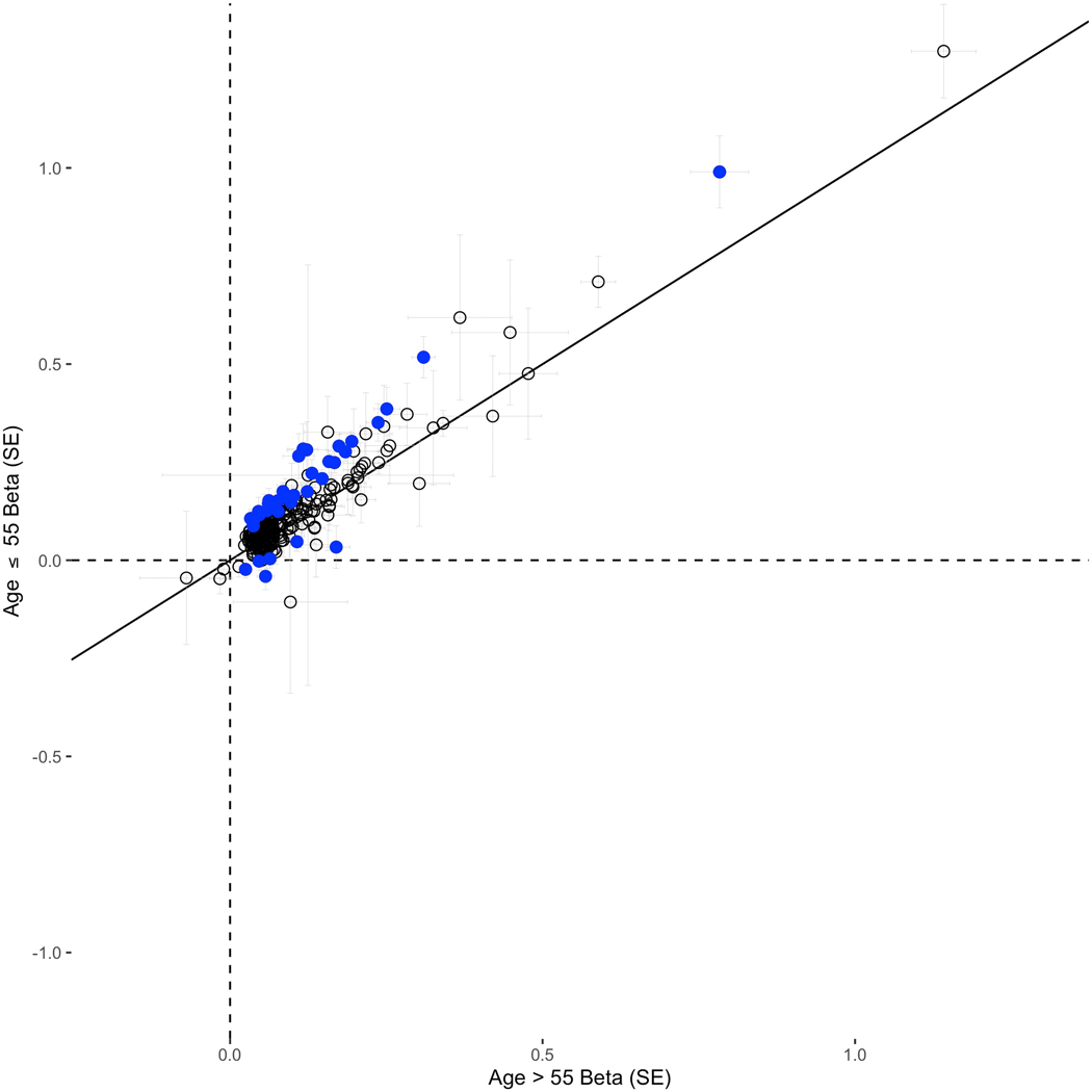
In multiancestry case-only analyses, 105 of the 269 risk variants were nominally associated (P < 0.05) with age at prostate cancer diagnosis (only three were nominally associated with older age at prostate cancer diagnosis), with 15 associated at P-value threshold < 5×10⁻⁸, including rs76765083 in KLK3 (0.78 years younger at diagnosis per allele, multiancestry P-value = 4.1×10⁻²⁰), rs10993994 upstream of MSMB (0.33, multiancestry P-value = 1.2×10⁻¹⁸), rs72725854 at 8q24 (1.46, African P-value = 7.1×10⁻¹⁵), rs183373024 at 8q24 (1.19, European P-value = 1.5×10⁻¹⁵) and HOXB13 variant rs138213197 (1.55, European P-value = 1.2×10⁻¹⁰) (Supplementary Table 7). In age-stratified case-control analyses, 188 of the 269 variants (69.9%) had larger effects in younger (≤55 years) compared to older (>55 years) men, 31 of which differed with a nominal P-value < 0.05 (Supplementary Table 8 and Extended Data 1).

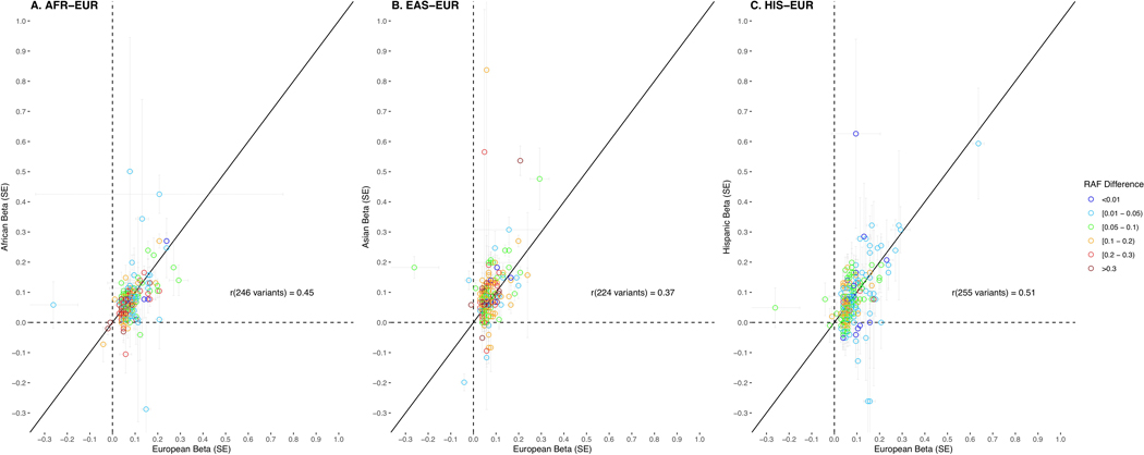
European versus African ancestry effect estimates (odds ratios) of the 269 risk variants were correlated with an r = 0.45, while European versus East Asian ancestry estimates were correlated at r = 0.37 and estimates for men of European ancestry versus Hispanic men were correlated at r = 0.51 (Extended Data 2). In comparing risk allele frequencies of the 269 risk variants across populations, average frequencies were similar between men of European ancestry (0.490), African ancestry (0.494) and Hispanic men (0.494) and were lowest in men of East Asian ancestry (0.479). However, variants with multiancestry odds ratios > 1.10 (71 variants, 26.4%) were on average more common in men of African ancestry (average risk allele frequency: 0.509 for men of African ancestry, 0.482 for men of European ancestry, 0.472 for men of East Asian ancestry and 0.483 for Hispanic men; Supplementary Table 9).

Based on a familial risk estimate of 2.5 for prostate cancer¹⁶, the 269 risk variants were estimated to capture 33.6% of familial relative risk (FRR) in men of East Asian ancestry, 38.5% in Hispanic men, 42.6% in men of European ancestry, and 43.2% in men of African ancestry (Supplementary Table 10). The 86 newly identified prostate cancer risk variants alone capture 5.4% of the FRR in men of European ancestry, 5.7% in both Hispanic men and men of East Asian ancestry, and 6.5% in men of African ancestry, which corresponds to 12.8–17.1% of the total FRR represented by the 269 risk variants.

Risk variant annotation.

In silico annotation of the 269 lead variants re-affirmed known prostate cancer susceptibility genes and identified a number of new strong candidate genes that may be involved in prostate tumorigenesis. (Supplementary Table 11). Fourteen of the lead variants are non-synonymous in 12 unique genes, two are situated in the 5’UTR and five in the 3’UTR of a gene, including a novel variant within the 3’UTR of the tumor suppressor TP53, for which a role in tumorigenesis is well established.¹⁷ We have also established the cancer-related 1100delC frameshift deletion in CHEK2 (NP_009125.1:p.Thr367fs)¹⁸ as a genome-wide significance risk variant for prostate cancer. A number of other lead variants demonstrate high or moderate evidence for regulatory potential, intersecting putative enhancer, repressor or promoter sites (Supplementary Table 11). For example, rs111595856 is located upstream of INHBB and is an expression quantitative trait loci (eQTL) for Inhibin subunit Beta B, a member of the transforming growth factor-beta superfamily involved in pituitary and gonadal hormone secretion and endocrine-related cancers, including prostate cancer.¹⁹ We observed overlap with a significant eQTL signal for 133 of the 269 lead variants (49.5%) in one or more prostate tissue datasets (Online Methods), including 36 of the 86 novel risk variants (41.9%), with 265 unique eGenes (genes for which expression is significantly associated with an eQTL) represented by the 133 lead variants (Supplementary Table 12). It is notable that of the 269 lead variants, 54 are situated within or adjacent to, or are associated with expression of, a transcription factor²⁰, of which seven are enriched in prostate tissue in the Human Protein Atlas.^21,22 An example includes SOX14 on chromosome 3, where the novel risk variant also intersects binding sites for regulatory factors AR, FOXA1 and HOXB13 involved in prostate cancer.

Developing genetic risk scores for prostate cancer.

To understand the aggregate effect of the 269 variants on prostate cancer risk, we constructed a genetic risk score (GRS) using the multiancestry weights of the risk variants associated with disease (Online Methods). Compared with men at average genetic risk in the 40–60% GRS category, the estimated odds ratio for men in the top 10% of the GRS (90–100% GRS category) was 5.06 [95% CI 4.84–5.29] for men of European ancestry, 3.74 [95% CI 3.36–4.17] for men of African ancestry, 4.47 [95% CI 3.52–5.68] for men of East Asian ancestry and 4.15 [95% CI 3.33–5.17] for Hispanic men (Table 2). Men in the top 1% of the GRS distribution (99–100%) had higher odds of disease, ranging from 11.65 [95% CI 10.56–12.85] for men of European ancestry to 5.68 [95% CI 4.44–7.28] for men of African ancestry. Category specific GRS risk estimates were very similar using weights from bias corrected estimates (Online Methods, Supplementary Table 13). GRS differences by population were comparable when using weights based on similar sample sizes of each population and equal weights for the 269 variants (Online Methods and Supplementary Table 14).

Table 2.

Genetic Risk Score (GRS) by Population.

	Multiancestry GWAS Sample Population Group								Replication Sample Population Group
GRS Category	European 71,570 cases, 52,531 controls		African 9,126 cases, 8,702 controls		East Asian 1,652 cases, 1,803 controls		Hispanic 2,226 cases, 2,098 controls		European (UK Biobank) 6,852 cases, 193,117 controls		African (CA UG) 1,586 cases, 1,047 controls
	OR	95% CI	OR	95% CI	OR	95% CI	OR	95% CI	OR	95% CI	OR	95% CI
0 – 10%	0.24	0.23 – 0.26	0.30	0.26 – 0.36	0.37	0.26 – 0.55	0.39	0.28 – 0.54	0.28	0.24 – 0.34	0.31	0.21 – 0.47
10 – 20%	0.42	0.40 – 0.45	0.52	0.45 – 0.60	0.48	0.34 – 0.68	0.59	0.44 – 0.79	0.40	0.35 – 0.47	0.49	0.34 – 0.71
20 – 30%	0.57	0.54 – 0.60	0.61	0.53 – 0.70	0.75	0.55 – 1.02	0.69	0.52 – 0.91	0.62	0.55 – 0.71	0.61	0.43 – 0.86
30 – 40%	0.73	0.69 – 0.77	0.77	0.67 – 0.87	0.76	0.56 – 1.03	0.80	0.61 – 1.05	0.79	0.70 – 0.89	0.72	0.52 – 1.01
40 – 60%	1.00	ref.	1.00	ref.	1.00	ref.	1.00	ref.	1.00	ref.	1.00	ref.
60 – 70%	1.36	1.29 – 1.42	1.43	1.27 – 1.60	1.25	0.95 – 1.65	1.46	1.15 – 1.87	1.29	1.17 – 1.43	1.45	1.07 – 1.97
70 – 80%	1.73	1.65 – 1.82	1.63	1.45 – 1.83	1.8	1.42 – 2.39	1.77	1.40 – 2.25	1.62	1.47 – 1.78	1.66	1.23 – 2.23
80 – 90%	2.45	2.34 – 2.56	2.37	2.12 – 2.65	2.37	1.84 – 3.06	2.47	1.97 – 3.11	2.43	2.23 – 2.65	1.78	1.32 – 2.40
90 – 100%	5.06	4.84 – 5.29	3.74a	3.36 – 4.17	4.47	3.52 – 5.68	4.15	3.33 – 5.17	4.17	3.85 – 4.51	3.53	2.66 – 4.69
99 – 100%	11.65	10.56 – 12.85	5.68a	4.44 – 7.28	9.41	5.60 – 15.82	6.85	4.20 – 11.18	9.03	7.87 – 10.35	7.05	3.66 – 13.56

^aP-value < 0.001 for heterogeneity testing for each GRS category versus men of European ancestry.

We examined GRS replication in two independent studies in men of European ancestry from the UK Biobank and in men of African ancestry from the California and Uganda (CA UG) study, neither of which were included in the multiancestry GWAS meta-analyses; additional studies in East Asian and Hispanic men are currently not available for GRS replication in these groups. The GRS associations with prostate cancer risk replicated in both men of European and African ancestry (Table 2). For men of European ancestry, the odds ratio was 4.17 [95% CI 3.85–4.51] for those in the top 10% of the GRS and 9.03 [95% CI 7.87–10.35] for those in the top 1%. For men of African ancestry, the odds ratio was 3.53 [95% CI 2.66–4.69] for those in the top 10% of the GRS and 7.05 [95% CI 3.66–13.56] for those in the top 1%.

The discriminative improvement of the GRS was evaluated in the UK Biobank using area under the curve (AUC). Compared to a model of age and family history (AUC = 0.784, 95% CI 0.779–0.789), incorporating the GRS into the model resulted in improved discrimination (AUC = 0.836, 95% CI 0.832–0.840, Δ = +0.052). Comparatively, a model of age and GRS (AUC = 0.833, 95% CI 0.828–0.837) was minimally improved upon incorporating family history (AUC = 0.836, 95% CI 0.832–0.840, Δ = +0.003; Online Methods and Supplementary Table 15). In the UK Biobank, relative to a model of age and family history, the addition of the GRS to the risk model also resulted in a 59.5% (95% CI 57.1–62.1%) net reclassification improvement (NRI), with similar improvement observed in both cases (29.4%, 95% CI 27.6–31.1%) and controls (30.2%, 95% CI 29.1–31.4%; Online Methods and Supplementary Table 15).

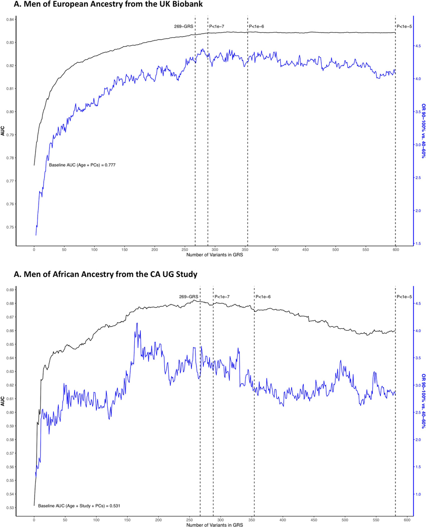
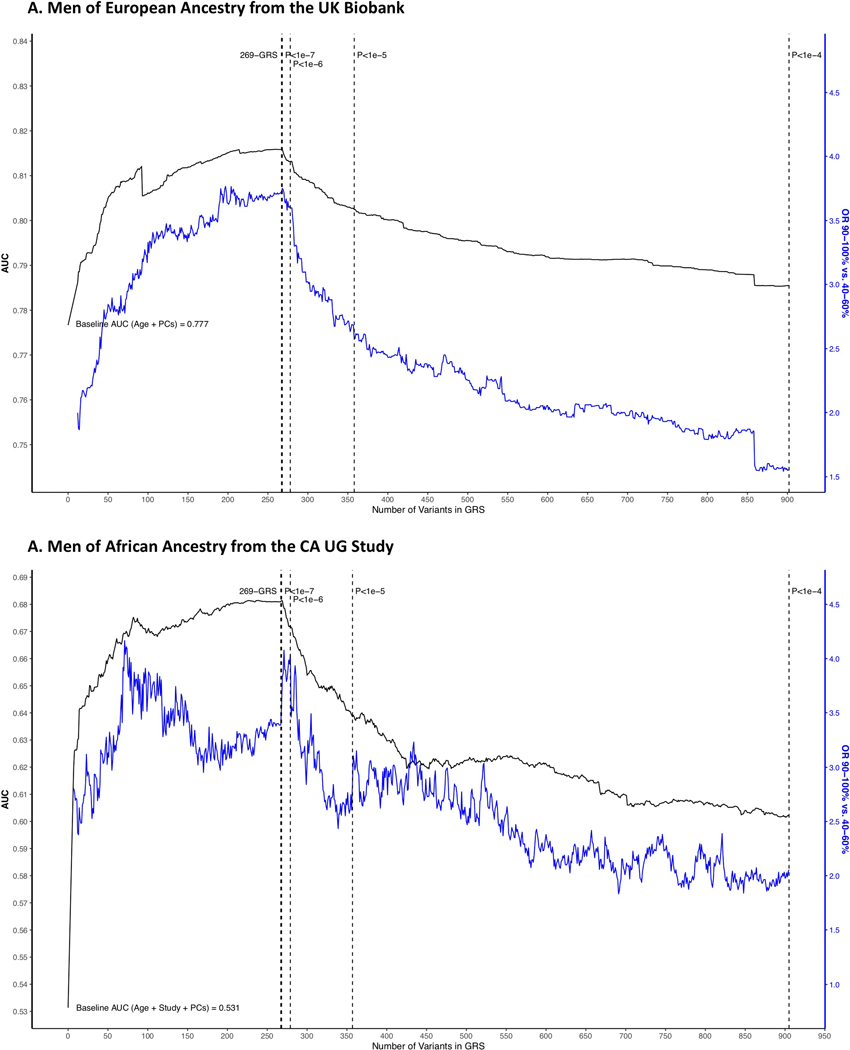
We also derived a genome-wide GRS that included the 269 genome-wide significant risk variants and additional variants independently associated (r² < 0.10 and > 800 kb from the 269 variants) with prostate cancer with a P-value < 1.0×10⁻⁵ from the multiancestry meta-analysis (605 total variants) (Online Methods). While effect sizes were typically larger for the genome-wide GRS than the 269-variant GRS in the discovery sample, associations with the genome-wide GRS and 269-GRS were similar in the replication studies of men of European ancestry from the UK Biobank and men of African ancestry from the CA UG study (Supplementary Table 15 and 16 and Extended Data 3). A genome-wide GRS was similarly constructed based on the African ancestry meta-analysis (917 total variants) (Online Methods); however, performance was poorer for men of both European and African ancestry (Supplementary Table 17 and Extended Data 4).

The relationship between GRS, age at diagnosis, family history and prostate cancer risk.

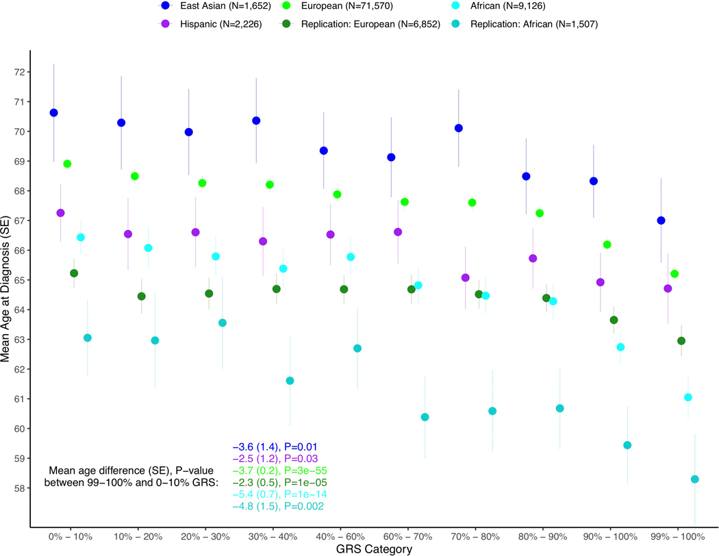
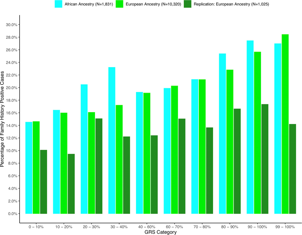
We found the GRS to be significantly associated with younger age at diagnosis in each population. Men with prostate cancer in the top 10% of the GRS distribution were diagnosed 2.84 years younger (95% CI −3.24, −2.44, P-value = 4.1×10⁻⁴⁴) on average, while men in the top 1% were diagnosed 3.88 years younger (95% CI −4.31, −3.44) on average than men in the bottom 10% across populations (Extended Data 5 and Supplementary Table 18). Men of both European and African ancestry with prostate cancer in the top 10% of the GRS were also 2.0-fold (95% CI 1.78–2.64, P = 1.4×10⁻¹⁴) more likely to have a first-degree family history of prostate cancer compared to men in the bottom 10% (Extended Data 6 and Supplementary Table 19).

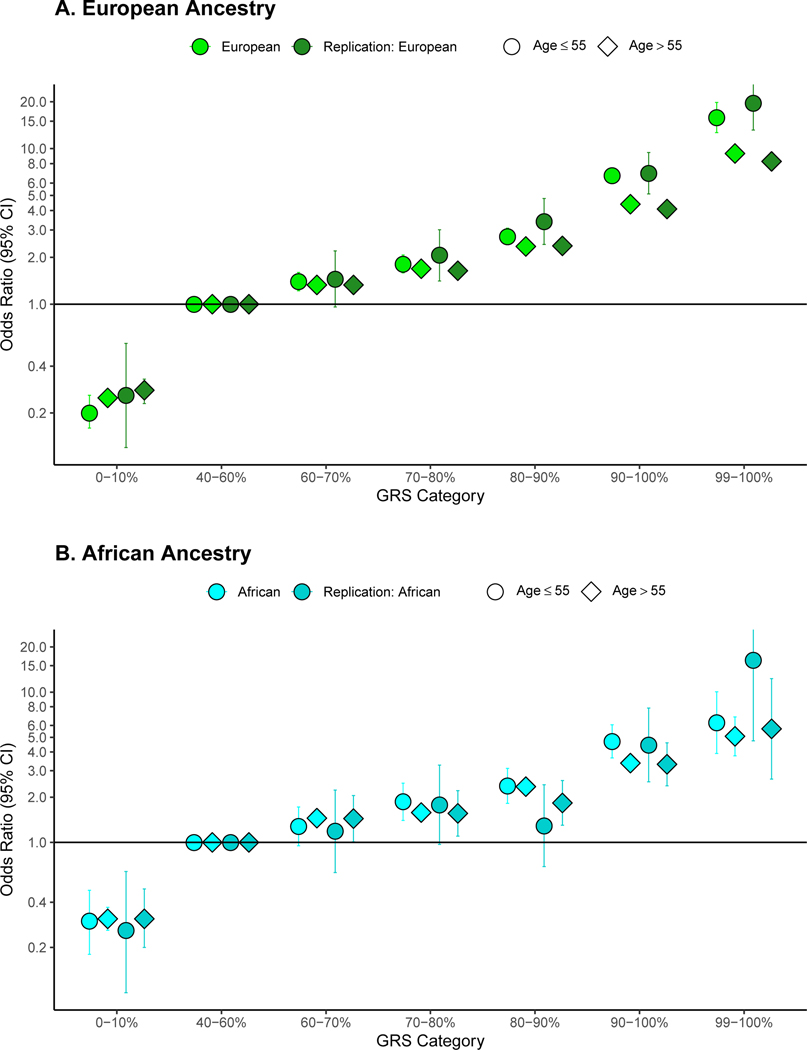
We also found age to modify the GRS association with prostate cancer risk for men in higher GRS categories (Supplementary Table 20). In men of European ancestry included in the GWAS meta-analysis (Fig. 1A), the top decile GRS category was associated with an odds ratio of 6.71 [95 % CI 5.99–7.52] for men ages 55 years or younger and 4.39 [95% CI 4.19–4.60] for men older than 55 years (P-heterogeneity for age = 1.5×10⁻¹¹). Effect modification of the GRS by age was similarly observed in men of African ancestry (P-heterogeneity = 0.02) and European ancestry men in the UK Biobank (P-heterogeneity = 0.004) (Fig. 1A, Fig. 1B and Supplementary Table 20). Odds ratios were even greater for the top 1% of the GRS (99–100% category) for younger men of European and African ancestry ages 55 years or younger (Fig. 1A and 1B). We did not observe evidence of effect modification of the top GRS decile by family history of prostate cancer in men of European or African ancestry (P-heterogeneity = 0.29 and 0.34, respectively; Supplementary Table 21).

Figure 1:

Odds ratio for prostate cancer by genetic risk score (GRS) category stratified by age. Results are shown for A. Men of European ancestry (N=124,101 from the genome-wide association study [GWAS] and 199,969 from independent replication) and B. Men of African ancestry (N=17,828 from the GWAS and 2,633 from independent replication). The x-axis indicates the GRS category [0–10% (low-risk), 40–60% (average risk), 60–70%, 80–90%, 90–100% (high-risk) and 99–100% (high-risk)]. The y-axis indicates odds ratios with error bars representing 95% confidence intervals (Cis) for each GRS category compared to the 40–60% GRS as the reference. The horizontal line corresponds to an odds ratio of one. Odds ratios and 95% CIs for each decile and strata are provided in Supplementary Table 20.

The relationship between GRS and disease aggressiveness.

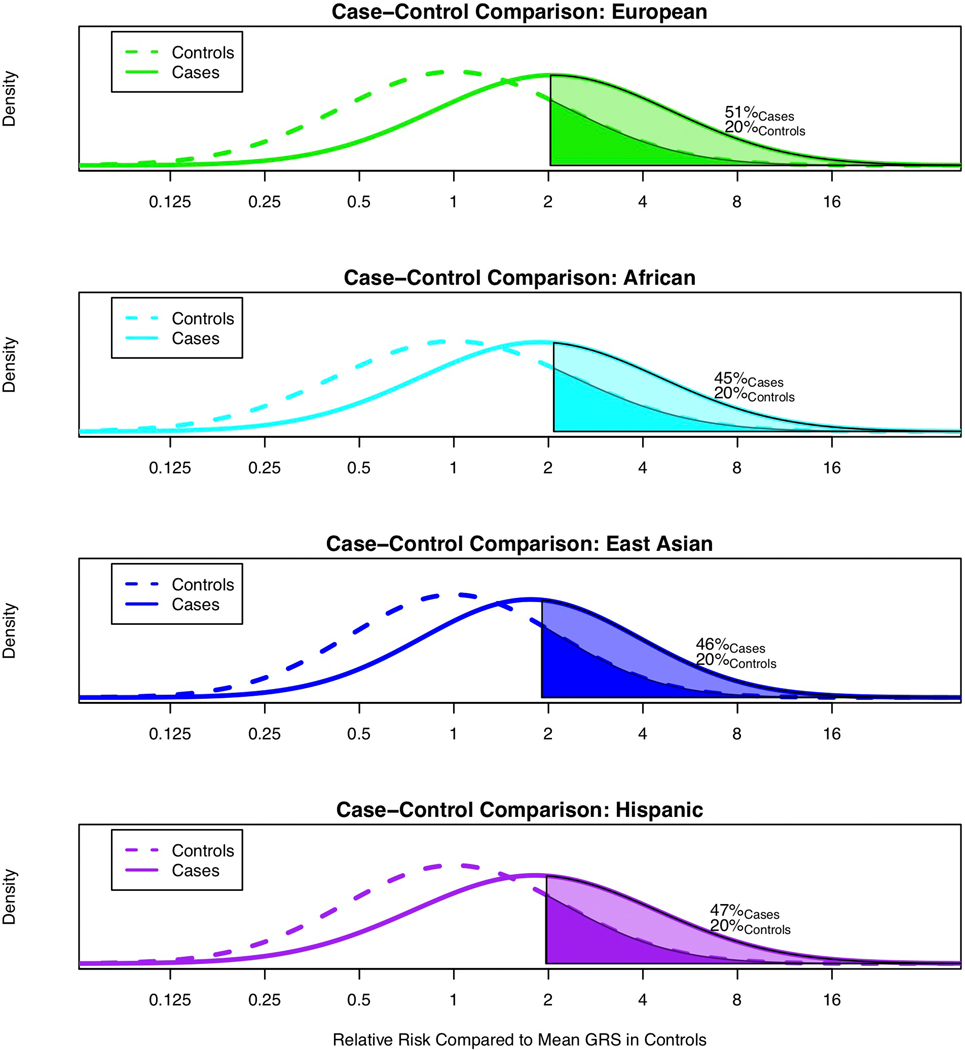
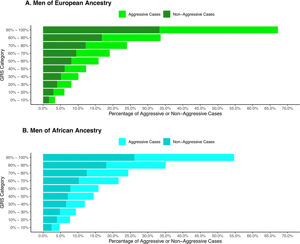
We observed no evidence of the GRS differentiating risk of aggressive versus non-aggressive prostate cancer (i.e. case-only odds ratios in each decile were ~1 and case-control odds ratios were similar for cases with non-aggressive and aggressive phenotypes versus controls in stratified analyses; Supplementary Table 22 and 23). However, 45–51% of all men with aggressive prostate cancer in these populations have a GRS in the top 20% (Extended Data 7 and 8). Thus, while the GRS does not predict who is more likely to develop aggressive disease (vs. non-aggressive disease), it can define a subset of men (i.e. 20% of the population) in which a substantial fraction of aggressive cases will develop.

Comparing GRS distributions across populations.

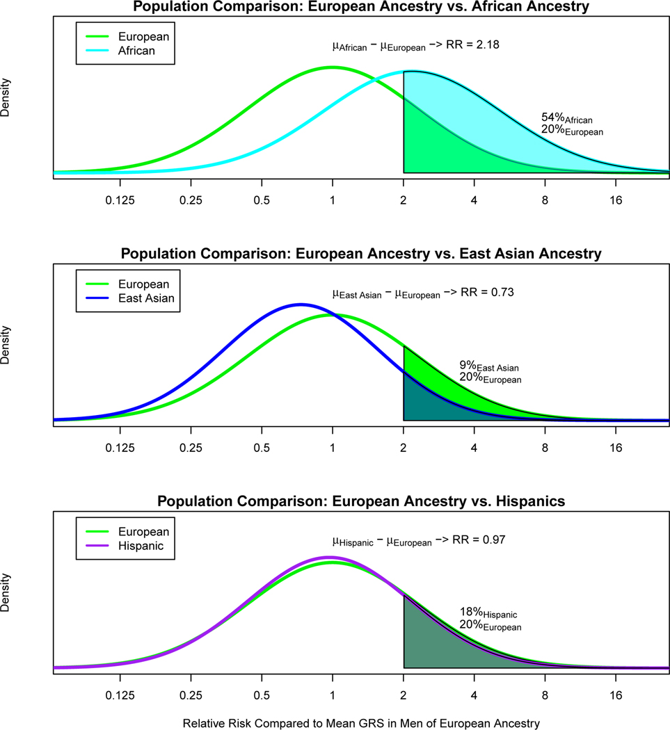
In comparing the GRS across populations, we found that the GRS distribution in controls was higher for men of African ancestry and lower for men of East Asian ancestry compared with men of European ancestry (Fig. 2). Relative to the mean prostate cancer GRS for men of European ancestry, 20% of men of European ancestry, 54% of men of African ancestry, 9% of men of East Asian ancestry and 18% of Hispanic men had a relative risk for the GRS greater than 2.0. Using the GRS distribution in controls, compared to the mean prostate cancer GRS in men of European ancestry, men of African ancestry had a mean prostate cancer GRS that was associated with a relative risk of 2.18 [95% CI 2.14–2.22], while Hispanic men and men of East Asian ancestry had relative risks of 0.97 [95% CI, 0.94–1.00] and 0.73 [95% CI 0.71–0.76], respectively. Within the admixed African and Hispanic populations, associations were similar in GRS analyses stratified by global European ancestry (Supplementary Table 24). All tests of heterogeneity had a P-value > 0.40 (Online Methods).

Figure 2.

Comparison of prostate cancer GRS distributions for controls. A. Men of European ancestry versus men of African ancestry; B. Men of European ancestry versus men of East Asian ancestry; and C. Men of European ancestry versus Hispanic men. The x-axis indicates the relative risk calculated by exponentiation of the difference in the mean GRS in controls for men of European ancestry and the mean GRS in controls for each of the other populations. The y-axis indicates the GRS density. Solid areas and corresponding percentages indicate the proportion of a given population with a relative risk greater than or equal to 2.0 in comparison to the mean GRS for men of European ancestry.

Estimating absolute risk of prostate cancer by GRS.

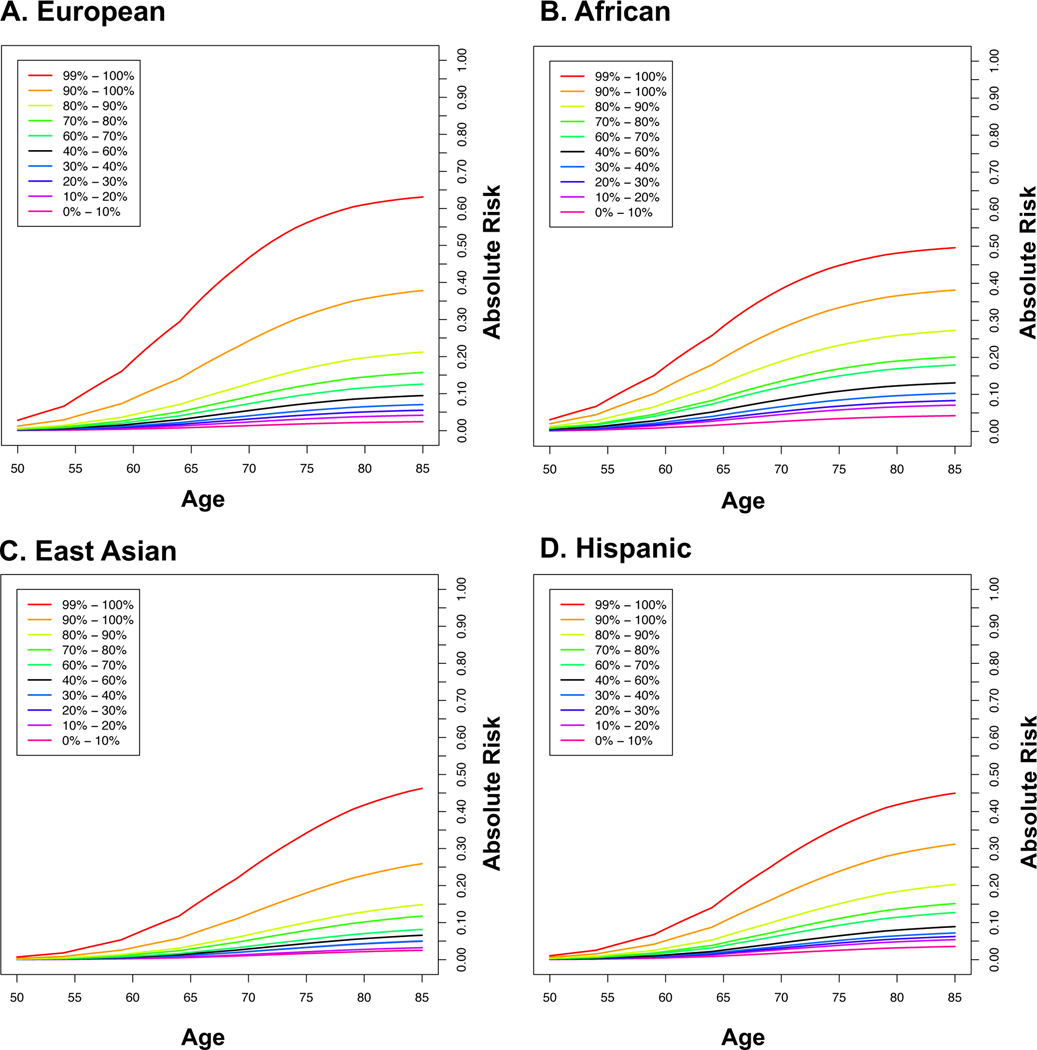
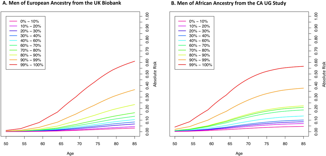
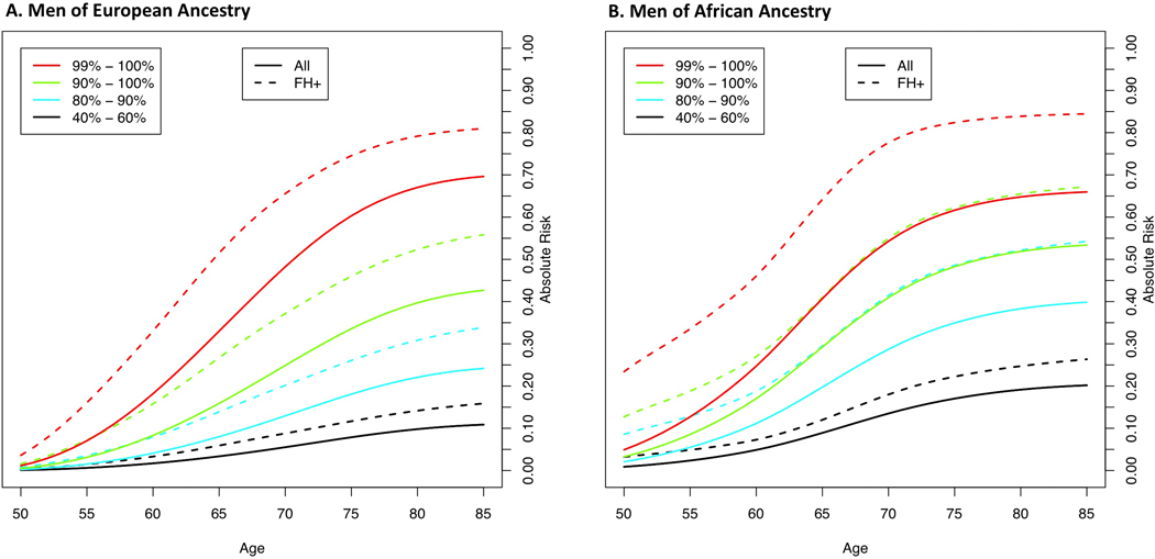
Lifetime absolute risks of prostate cancer by GRS category and ancestry group are shown in Fig. 3 (Supplementary Table 25). The absolute risk for men in the top decile of the GRS reached 38% for both men of African [95% CI 36%−41%] and European [95% CI 37%−39%] ancestry, 31% [95% CI 27%−36%] for Hispanics and 26% [95% CI 22%−30%] for East Asians. Absolute risk estimates were only slightly reduced when using GRS estimates from men of European and African ancestry in the UK Biobank and CA UG replication studies, respectively (Extended Data 9 and Supplementary Table 25). Men with a first-degree family history of prostate cancer had increased absolute risks for each GRS category, with 67% [95% CI 59%−76%] and 56% [95% CI 52%−60%] lifetime absolute risks estimated for men in the top 10% for African and European ancestry men, respectively (Supplementary Table 26 and Extended Data 10).

Figure 3.

Absolute risks of prostate cancer by GRS category. A. European ancestry; B. African ancestry; C. East Asian ancestry; and D. Hispanic. SEER data is used for mortality and incidence rates corresponding to non-Hispanic White, Black, Asian and Hispanic men. The x-axis indicates the age of an individual and the y-axis is the absolute risk by a given age.

Discussion

Through this large multiancestry GWAS meta-analysis, we identified 86 novel risk variants that influence prostate cancer susceptibility and point to a number of novel candidate genes potentially involved in prostate cancer development. We integrated these discoveries with known risk loci for prostate cancer to derive a GRS based on 269 risk variants for prostate cancer that could effectively stratify prostate cancer risk across populations, with GRS associations replicating in two independent studies in men of European and African ancestry.

The inclusion of non-European ancestry samples, especially those of African ancestry, allows for better refinement of signal(s) within regions.²³ However, the discovery of novel variants and lead variants in known regions was largely determined by the size of the European ancestry sample, which represented 79.8% of the cases included in the GWAS. The smaller sample size of the African, Hispanic and East Asian studies resulted in an imbalance in the discovery of risk variants and in the precision of risk estimation in these groups. Because of this, for each variant, we used the multiancestry weight in the GRS estimation, as the effect is likely to more closely reflect that of the underlying causal allele, assuming little or no effect heterogeneity by population. While inflation of the GRS associations could result from using the same sample for risk variant discovery as GRS testing, the GRS predictive ability was comparable in the independent UK Biobank and CA UG studies, and sensitivity analyses incorporating weights with a bias correction had little impact on GRS associations.

Despite population sample size differences, the magnitudes of GRS associations were similar across populations, except for men of African ancestry, in which the odds ratio in the top GRS decile was attenuated by ~20% for men of African ancestry compared to men of European ancestry. This consistency of GRS performance across ancestral populations has not generally been observed for GRS derived for cancers or many other diseases or traits²⁴ and is likely the result of prostate cancer having a strong genetic component, the multiancestry approach we employed, which allowed for the discovery of novel pan-ancestry variants and the refinement of lead variants in known risk regions, and the use of multiancestry weights in the GRS. However, GRS distributions were observed to vary widely across populations, signifying the importance of incorporating an individual’s ancestry before GRS-associated risk can be assigned to an individual, particularly for admixed populations.

While larger GRS effect sizes were observed in men of European ancestry, the greater disease incidence for men of African ancestry resulted in our reporting comparable lifetime risk estimates for GRS deciles. Ancestry-specific GRS cutoffs were used to determine the 10% of men in each population at highest risk, who had estimated lifetime risks of developing prostate cancer that ranged from 38% for African and European ancestry men, 31% for Hispanic men and 26% for East Asian men. Estimated lifetime risks for men in the top GRS decile were > 50% for African and European ancestry men who also had a family history of prostate cancer.

We found little evidence that a genome-wide GRS improved risk prediction beyond the 269-variant GRS. Of the 269 variants, those with odds ratios > 1.10, which have a larger contribution to the GRS than variants with weaker effects (odds ratios ≤ 1.10), were more common in men of African ancestry, resulting in a greater contribution of the GRS to the overall risk of prostate cancer for this ancestry group. Based on our observed 2-fold difference in the mean GRS distribution in controls between men of European and African ancestry, in aggregate, the known risk variants are estimated to account for a substantial fraction of the ~70% greater prostate cancer incidence observed in men of African ancestry. However, it will be important to incorporate the biologically functional variants and local ancestry differences in order to better understand how GRS distributions relate to population differences in prostate cancer incidence.

For men between 55 and 69 years of age, the U.S. Preventive Task Force recommends that the decision to undergo PSA screening should be an individual one, following consultation with a physician and considering information about family history of prostate cancer and African ancestry.²⁵ Currently, genetic information is not incorporated into the decision-making process for PSA screening. However, men with a high GRS may benefit from earlier and more frequent screening, while knowledge of a low GRS may help to reduce unnecessary biopsies for men with borderline screening PSA levels. While the lifetime risk of developing prostate cancer is heavily dependent on age, the odds ratio associated with the top GRS decile was greater for younger compare to older men. For cancer, younger age at diagnosis typically indicates a genetic influence on disease onset, which is supported by our findings of common genetic variants having a greater impact on prostate cancer risk for earlier versus later onset disease. As such, regular PSA screening may be beneficial even earlier than age 55 for a subset of men at high genetic risk.

Consistent with previous findings, we found that common variants are equally associated with risk of aggressive and non-aggressive prostate cancer. Although we found little evidence that the GRS can differentiate risk of aggressive versus non-aggressive disease, the GRS could define ~20% of men in each population at high risk, which includes one-half of the men who will be diagnosed with aggressive disease. While the benefit/harm tradeoffs of including GRS in future risk-tailored screening programs need to be evaluated, these data suggest that GRS greatly improves upon discriminative models based on age and family history and that a substantial fraction of men who will develop aggressive tumors may be identified earlier through risk-based screening.

In summary, we have applied a multiancestry approach to discover novel risk variants for prostate cancer, refine lead variants in known risk regions and develop a GRS for prostate cancer that is effective in stratifying prostate cancer across populations. These findings also provide further support for a contribution of germline variation to ancestry differences in prostate cancer incidence. The clinical benefit of GRS profiling for targeted screening and early diagnosis needs to be examined, and larger prostate cancer consortia in men of non-European ancestry, particularly in men of African ancestry, will be required to identify additional risk variants, improve precision of risk estimation and enhance the predictive ability of the GRS across populations.

Online Methods

Study Subjects in the Multiancestry GWAS.

This investigation includes the Prostate Cancer Association Group to Investigate Cancer-Associated Alterations in the Genome and Collaborative Oncological Gene-Environment Study Consortium (PRACTICAL iCOGS), the Elucidating Loci Involved in Prostate Cancer Susceptibility OncoArray Consortium (ELLIPSE OncoArray), the United Kingdom GWAS (UK GWAS1 and UK GWAS2), Cancer of the Prostate in Sweden (CAPS1 and CAPS2), the National Cancer Institute (NCI) Prostate cancer Genome-wide Association Study of Uncommon Susceptibility loci study (PEGASUS), the NCI Breast and Prostate Cancer Cohort Consortium (BPC3), the ProHealth GWAS Study within the Research Program on Genes, Environment and Health Kaiser Permanente cohort (ProHealth Kaiser GWAS), the African Ancestry Prostate Cancer Consortium (AAPC GWAS), BioBank Japan (RIKEN GWAS1 and GWAS2), GWAS of prostate cancer in Latinos (LAPC GWAS) and Japanese (JAPC GWAS) in the Multiethnic Cohort Study (MEC) and the Ghana Prostate Study (GPS). In total, 136 studies contributed samples and/or summary statistics to the analysis. An overview of each study is provided in Supplementary Table 1. Informed consent was obtained from all participants and study protocols were approved by respective Institutional Review Boards.

Genotyping and Imputation in the Multiancestry GWAS.

The genotyping array, sample and variant quality control, imputation and the basic statistical software used for each study or consortium are summarized in Supplementary Table 2. Details for each individual study or consortium have been described elsewhere (see references in Supplementary Table 1). In general, samples and variants were excluded with a corresponding study-specific sample or genotyping call rate < 95%. Most studies limited variants analyzed to those with a MAF ≥ 1%, although there were exceptions, including the ELLIPSE OncoArray Consortium that included all variants. Most studies screened variants with a test of Hardy-Weinberg equilibrium (with varying significance thresholds), but a few studies did not implement such a screen. Imputation used either MACH²⁶, Minimac3/Minimac4²⁷ or IMPUTE2²⁸ using Phase 3 of the 1000 Genomes Project¹⁵ as the reference panel. Post-imputation variant inclusion criteria included MAF ≥ 1% and an imputation INFO/r² ≥ 0.3.

Study Subjects Included in GRS Replication.

We used GWAS data for 199,969 men of European ancestry from the UK Biobank (https://www.ukbiobank.ac.uk), which included 6,852 cases and 193,117 controls (Supplementary Table 1 and 2). Genotype data was generated in the UK Biobank using the Affymetrix UK Biobank Axiom Array and the Affymetrix UK BiLEVE Axiom Array and imputation was performed using the Haplotype Reference Consortium (HRC), UK10K and 1000 Genomes Project panels.²⁹ All samples had GWAS data, were genetically identified as male, did not have high heterozygosity or missingness prior to imputation, and were unrelated (2nd degree or higher relationships with a kinship > 0.0884 were excluded).

For men of African ancestry, GRS replication was conducted among 1,586 cases and 1,086 controls from California and Uganda (CA UG Study) genotyped with the Illumina H3 Africa array and imputed using Phase 3 of the 1000 Genomes Project¹⁵ as the reference panel and Minimac4 on the Michigan Imputation Server²⁷ (Supplementary Table 1 and 2). All samples were genetically identified as male, had a genotyping call rate ≥ 95%, and were unrelated to men in our multiancestry GWAS meta-analysis.

Statistical Analysis for GWAS.

Genetic ancestry was estimated using a principal component analysis performed in each study based on uncorrelated single nucleotide polymorphisms (SNPs). Ancestry was based on self-report with extremely admixed individuals (e.g. ± 4SD outside of ancestry-specific clusters defined with principal components) removed for non-Hispanic population-specific analyses. In total, 29,235,255 variants (SNPs and indels) on autosomal chromosomes 1–22 and the X chromosome were examined for association with prostate cancer risk using logistic regression adjusting for age, sub-study (described in Supplementary Table 1) and principal components with PLINK³⁰, SNPtest³¹, or R. Per-allele odds ratios and standard errors from individual studies were combined by a fixed-effects inverse-variance weighted meta-analysis using METAL³² in ancestry-specific analyses and across all four populations to obtain multiancestry estimates. All statistical tests conducted were two-sided. A marginal P-value less than 5.0×10⁻⁸ in either the population-specific or multiancestry analysis was used to define statistically significant genetic associations, with regions bounded within +/− 800 kb from the most significant variant. To determine if multiple independent associations exist within each region, we implemented a forward stepwise selection starting with the inclusion of the lowest multiancestry marginal P-value into a multivariate logistic regression model. We used Joint Analysis of Marginal summary statistics (JAM)³³ to obtain population-specific conditional summary statistics from multivariate models. Conditional statistics were combined with an inverse-variance weighted fixed effects meta-analysis to obtain multiancestry conditional summary statistics (Supplementary Table 4). Variants with a conditional multiancestry P-value < 5.0×10⁻⁸ were retained in the model. We excluded variants with a marginal multiancestry P-value > 5.0×10⁻⁴, MAF < 1% in all four populations, and correlation r² ≥ 0.2 to any variants included in the current model at each step. Poorly imputed selected variants (n=8) were replaced with suitable surrogate variants with imputation scores > 0.8 across studies and populations (Supplementary Table 5).

We conducted stratified case-control and case-case analyses to evaluate the impact of the novel variants on disease aggressiveness (Supplementary Table 6). As previously defined⁴, aggressive prostate cancer (i.e. high-risk) was defined as tumor stage T3/T4, regional lymph node involvement, metastatic disease, Gleason Score ≥ 8, prostate-specific antigen (PSA) level ≥ 20 ng/mL or prostate cancer as the underlying cause of death and non-aggressive disease (i.e. intermediate and low-risk) was defined as Gleason ≤ 7, PSA < 20 and stage ≤ T2. Studies missing these clinical features were excluded (Table 1).

Genetic Risk Score (GRS) Construction.

Genetic risk scores (GRS) were constructed using all studies with individual-level data (Supplementary Table 1) by summing variant-specific weighted allelic dosages. The initial GRS included the 269 risk variants, including established rare (<1% frequency) moderate penetrance risk variants at 8q24 (rs183373024)⁹, HOXB13 (rs138213197, NP_006352.2:p.Gly84Glu)³⁴ and CHEK2 (c.1100delC, rs555607708, NP_009125.1:p.Thr367fs)³⁵ (Supplementary Table 4). Specifically, for individual i, ${GRS}_i=\sum _{m=1}^M{w}_m{g}_{im}$, where $g_{im}$ is the genotype dosage for individual i for variant m and $w_m$ is a variant-specific weight (on the log odds ratio scale) calculated by meta-analyzing the ancestry-specific conditional effects from the JAM analysis using an inverse Z-score weighted fixed effects meta-analysis. An inverse Z-score weight was used rather than an inverse variance weight to up-weight noteworthy population-specific variants that may not have evidence in other populations. M is the total number of variants included.

The risk of the GRS on prostate cancer was estimated using indicator variables for the percentile categories of the GRS distribution: [0–10%], (10–20%], (20–30%], (30–40%], (40–60%], (60–70%], (70–80%], (80–90%], and (90–100%]. An additional analysis was also performed by splitting the top decile into two categories to obtain the GRS risk for the top 1%: (90–99%], (99–100%]. GRS thresholds were determined using the observed distribution among controls for the corresponding ancestry group. Logistic regression was used to estimate odds ratios corresponding to each GRS category, adjusting for principal components, age and sub-study, using the (40–60%] category as the reference. To obtain ancestry-specific GRS estimates, an inverse-variance weighted fixed effects meta-analysis was performed within each population. Multiancestry estimates were obtained via an inverse-variance fixed effects meta-analysis using the ancestry-specific results.

GRS Replication Analysis.

We examined the GRS in men of European ancestry in the UK Biobank and African ancestry in the CA UG study; additional studies in East Asian and Hispanic men are currently unavailable. Of the 269 risk variants, 267 were present in the UK Biobank sample, all of which had an imputation info score > 0.50 (median info score=0.99), and 266 were present in the CA UG Study and had an imputation info score > 0.36 (median info score=0.98). The GRS used the multiancestry conditional weights from the previous GRS analysis. Odds ratios were estimated within populations comparing each GRS decile to the 40–60% category using logistic regression models adjusted for age, ten principal components and sub-study (African American vs. Ugandan in the CA UG study). GRS models were further evaluated in analyses stratified by age, as described below.

Bias Correction and Sensitivity Analysis for GRS.

Since a subset of the data used in the overall multiancestry meta-analysis was initially used to evaluate the GRS, there is the potential for bias to exist in GRS estimates from these data (note that this does not apply to replication analyses, which were performed in independent samples). As shown in Zhong and Prentice,^36,37 this bias becomes very small as the sample size increases. Given the overall sample size contributing to the multiancestry GWAS, bias potential exists only for very small true variant effects. To correct for this potential bias, the variant-specific weights used in our primary GRS analysis (i.e. the weights from the multiancestry meta-analysis of ancestry-specific conditional JAM effects) were corrected using the approach outlined Zhong and Prentice³⁶ and used to construct a second GRS to investigate this potential bias (Supplementary Table 13).

To investigate the influence of the large sample of European ancestry men on GRS weights, we recalculated weights for the 269 variants limiting the number of European ancestry men to 10,000 cases and 10,000 controls (roughly the same size as the African ancestry sample). Resulting weights were highly correlated with original weights (r²=95.1%). These weights were used to calculate a GRS, and the association between this GRS and prostate cancer was evaluated. We also developed an equally weighted GRS using the average conditional effect of the 269 variants and evaluated the association between this GRS and prostate cancer.

Discriminative Improvement of GRS.

The discriminative improvement of the GRS was evaluated in men of European ancestry from the UK Biobank using area under the curve (AUC) and net reclassification improvement (NRI). AUCs were calculated using four separate logistic regression models of prostate cancer, which included the following variables: 1) age, 2) age and family history of prostate cancer, 3) age and GRS and 4) age, family history and GRS. Each model was additionally adjusted for ten principal components of ancestry. NRI indicates the amount of reclassification improvement of cases and controls resulting from the addition of a variable to a model.³⁸ NRI was calculated comparing model 2 (age and family history) and model 4 (age, family history and GRS), both of which additionally included ten principal components. These calculations were based on the continuous NRI model, suggested by Pencina et al.³⁸ to be the most versatile measure of improvement in risk prediction and appropriate for case-control data. The 95% confidence intervals for NRI estimates were calculated using 1,000 bootstrap replications.

Expanded Genome-Wide GRS.

A genome-wide GRS was developed using 605 variants independently associated (r² < 0.10) with prostate cancer risk at a multiancestry P-value < 1.0×10⁻⁵, which included the 269 risk variants and excluding variants within 800 kb of these 269 variants. Independence was determined using PriorityPruner (prioritypruner.sourceforge.net) and the 1000 Genomes Project¹⁵ reference populations, first identifying independent variants within the AFR, followed by EUR, EAS and AMR populations. Variants with an imputation info score < 0.30 were excluded, as were variants with a MAF < 1% in all four discovery populations. The GRS was constructed using the same individual-level data used in the genome-wide significant GRS, summing allelic dosages weighted by variant-specific marginal multiancestry weights. Odds ratios were estimated for each GRS decile relative to the average 40–60% category, adjusting for principal components, age and sub-study. Ancestry-specific GRS estimates were obtained using an inverse-variance weighted fixed effects meta-analysis performed within each population, and multiancestry estimates were obtained using an inverse-variance fixed effects meta-analysis performed across the ancestry-specific results. For comparison, we also calculated the genome-wide GRS using subsets of these variants with a multiancestry GWAS meta-analysis P-value < 1.0×10⁻⁶ and P-value < 1.0×10⁻⁷, retaining the 269 variants in each. We also calculated the AUC and odds ratio for the 90–100% versus 40–60% GRS categories upon iteratively adding each variant to the GRS, first adding the most significant variants within the list of 269 followed by our identified genome-wide variants, sorted by their multiancestry GWAS meta-analysis P-values.

This process was repeated to develop and test an African ancestry-based genome-wide GRS using 917 variants independently associated (r² < 0.10) with prostate cancer risk at an African ancestry P-value < 1.0×10⁻⁴ (this larger P-value was used to identify a comparable number of variants), also retaining the 269 variants. African ancestry variant-specific weights were used in the African ancestry genome-wide GRS.

Stratification of Risk Estimation for GRS.

We investigated the GRS effect stratified by age and first-degree family history of prostate cancer and its association with aggressive disease phenotypes, including Gleason Score and metastatic disease (Supplementary Tables 20–23). For age and family history, cases and controls were stratified into age groups (age ≤ 55 vs. age > 55) or family history positive vs. negative. For aggressive disease strata, cases were stratified by disease aggressiveness and corresponding stratified analyses used all controls. Stratified analyses were also performed comparing aggressive cases to non-aggressive cases. Logistic regression was performed with prostate cancer status (either case vs. control or aggressive vs. non-aggressive) as the outcome and GRS categories as the independent predictors, adjusting for principal components, age and sub-study. Ancestry-specific GRS estimates were obtained via an inverse-variance weighted fixed effects meta-analysis performed within each population. Overall multiancestry estimates were obtained via an inverse-variance fixed effects meta-analysis using ancestry-specific results (European and African only). The sample sizes of the other populations (East Asian and Hispanic) were too small for stratified analyses. Heterogeneity was assessed via a Q-statistic between effect estimates with corresponding tests of significance.

We also estimated the GRS effect stratified by global ancestry in African and Hispanic populations, given the high admixture of these populations, using logistic regression models adjusted for age, sub-study and principal components (Supplementary Table 24). Global ancestry estimates were calculated as previously described⁶ using RFMix³⁹ and the 1000 Genomes data.¹⁵ African and Hispanic populations were stratified by their median percentages of global European ancestry (15% and 58%, respectively). Analyses were also performed stratifying Hispanic men by their median percentage of global Amerindian ancestry (37%). Heterogeneity was assessed to determine whether effects differed between those with more versus less European or Amerindian ancestry by adding to logistic regression models an interaction term between the continuous GRS and dichotomized ancestry indicator.

Estimation of Relative Risk for Ancestry.

To estimate the relative risk between ancestry groups due to the GRS, we used the distributions of the GRS in controls across the four populations. As the GRS is calculated on the log odds scale, we can estimate the relative risk between any two populations as the exponential of the difference between the corresponding mean GRS distributions in controls. Specifically, the relative risk comparing population a vs. population b is given by: ${RR}_{\text{a}\text{vs.}\text{b}}=\text{exp}\left[\mathrm{l}\mathrm{o}\mathrm{g}\left(\frac{a}{b}\right)\right]=\exp \left[\log \left(a\right)-\log \left(b\right)\right]=\text{exp}\left[{\mu }_{GRS}^a-{\mu }_{GRS}^b\right]$, where ${\mu }_{GRS}^a$ is the mean GRS in population a. As the difference in means can be viewed as a two-sample test, corresponding standard errors and confidence intervals were calculated in a similar fashion as a two sample t-test with unequal variance using the observed population means, ${\mu }_{GRS}^a$, standard deviations, ${\sigma }_{GRS}^a$, and corresponding sample sizes for controls.

Age-Specific Absolute Risk Estimation.

As an alternative way to investigate the impact of the GRS, we calculated the absolute risk for a given age for each GRS category and each ancestry.^40–43 The approach constrains the GRS-specific absolute risks for a given age to be equivalent to the age-specific incidences for the entire population. In other words, age-specific incidence rates are calculated to increase or decrease based on the GRS category estimated risk and the proportion of the population within the GRS category. The calculation accounts for competing causes of death.

Specifically, for a given ancestry group and a given GRS risk category k (e.g. 80–90%, 90–100%), the absolute risk by age t is computed as: ${AR}_k\left(t\right)={\sum }_0^t{P}_{ND}\left(t\right)S_k\left(t\right)I_k\left(t\right)$. This calculation consists of three components:

1. $P_{ND}\left(t\right)$ is the probability of not dying from another cause of death by age t using age-specific mortality rates, ${\mu }_D\left(t\right)$: $P_{ND}\left(t\right)=\text{exp}\left[-{\sum }_0^t{\mu }_D(t-1)\right]$. Age-specific mortality rates are provided from a reference cohort.

2. $S_k\left(t\right)$ is the probability of surviving prostate cancer by age t in the GRS category k and uses the prostate cancer incidence by age t for category k: $S_k\left(t\right)=\text{exp}\left[-{\sum }_0^t{I}_k(t-1)\right]$.

3. The prostate cancer incidence by age t for GRS category k is $I_k\left(t\right)$ and is calculated by multiplying the population prostate cancer incidence for the reference category, $I_0\left(t\right)$ and the corresponding risk ratio for GRS category k, as estimated from the odds ratio obtained from the population-specific individual-level GRS analysis as described above: $I_k\left(t\right)=I_0\left(t\right)\mathrm{e}\mathrm{x}\mathrm{p}\left({\beta }_k\right)$.

Prostate cancer incidence for age t for the reference category, $I_0\left(t\right),$ is obtained by constraining the weighted average of the population cancer incidences for the GRS categories to the population age-specific prostate cancer incidence, $\mu \left(t\right)$. $I_0\left(t\right)=\mu \left(t\right)\frac{\sum _K{f}_k{S}_k(t-1)}{\sum _K{f}_k{S}_k(t-1)\mathrm{e}\mathrm{x}\mathrm{p}\left({\beta }_k\right)}$, where $f_k$ is the frequency of the GRS category k with $f_k=0.1$ for all non-reference categories in our primary GRS analysis by deciles (e.g. [0–10%], (10–20%], (20–30%], etc.).

By leveraging the definition that $S_k\left(t=0\right)=1$, for all k, the absolute risks were calculated iteratively by first getting $I_0\left(t=1\right)$, then $I_k\left(t=1\right)$, then $S_k\left(t=1\right)$ and finally ${AR}_k\left(t=1\right)$. Subsequent values were then calculated recursively for all t. Confidence intervals for absolute risk estimates were obtained via a parametric bootstrap repeating the above calculations for 1,000 bootstraps with the ${\beta }_k$’s sampled from their corresponding estimated distributions using the standard error of the estimate.

For each ancestry group, absolute risks by age t were calculated using age-specific prostate cancer incident, $\mu \left(t\right)$, from the Surveillance, Epidemiology, and End Results (SEER) Program (1999–2013)¹⁰ and age-specific mortality rates, ${\mu }_D\left(t\right)$, from the National Center for Health Statistics, CDC (1999–2013).¹¹ Using the same analytic framework, absolute risks were also calculated using the family history stratified estimates for the GRS combined with mortality and incident rates estimated from men from the Multiethnic Cohort (MEC) with a positive family history of prostate cancer. Rates were based on 35,711 White and African American men and 4,060 incident cases identified over a 20-year period (1993–2013). For absolute risks in those with a positive family history, the log odds ratio estimates, ${\beta }_k$, were obtained from the corresponding stratified analysis.

Proportion of familial risk explained.

The contribution of the 269 variants to the familial risk (i.e. sibling recurrence risk) of prostate cancer was computed using the formula: $\frac{\sum _k\left(log{\lambda }_k\right)}{\left(log{\lambda }_0\right)}$, where λ₀ is the observed familial risk to first degree relatives of prostate cancer cases, assumed to be 2.5¹⁶, and λ_k is the familial relative risk (FRR) due to locus k, given by: $\lambda =\frac{p_k{r}_k^2+q_k}{(p_k{r}_{k+q_k}{)}^2}$, where p_k is the frequency of the risk allele for locus k, q_k = 1 – p_k and r_k is the estimated per-allele odds ratio.^44,45

In Silico Annotation.

The 269 risk variants were annotated for putative evidence of biological functionality (Supplementary Table 11) using publicly available datasets according to the framework described by Dadaev et al.⁷

Variants were annotated for genomic context and proximity to genes (ENSEMBL/Gencode definitions) using wANNOVAR⁴⁶, with additional manual review of exonic variants. Annotation of variants against intersection with chromatin marks indicative of regulatory DNA regions were performed relative to peak data from publicly available datasets generated in the prostate derived cell-lines LNCaP, PC3, PrEC and VCaP. Peak data were analyzed according to a standardized pipeline and QC procedures were downloaded from the Cistrome Data Browser⁴⁷ (http://cistrome.org/db/) and converted from GRCh38 to GRCh37/hg19 reference assembly co-ordinates in R using rtracklayer v1.42.2 liftOver.⁴⁸ Variants were assessed for intersection within DNaseI hypersensitivity site peaks in three datasets (GSM1024742, GSM736565 and GSM822387) and ATAC-seq peaks in three datasets (GSM2186481, GSM3075372 and GSM3075374). Histone modification site data was obtained for H3K27Ac (GSM1249447, GSM1249448 and ENCSR826UTD_1), H3K9Ac (GSM2527582 and GSM2527583), H3K4me1 (GSM1145323 and GSM2187238), H3K4me2 (GSM353635 and GSM1891829) and H3K4me3 (GSM1383874 and GSM945240). Transcription factor-binding site ChIP-seq peak data were obtained for the Androgen Receptor (GSM1274871, GSM1576447 and GSM1527834), CTCF (GSM1006874 and GSM2825574), ERG (GSM1193657 and GSM1328978), FOXA1 (GSM1274873, GSM1691142 and GSM2219863), GABPA (GSM1193660), GATA2 (GSM941195 and GSM1600544), HOXB13 (GSM1716764 and GSM2537218), NKX3.1 (GSM989640) and POLR2A (GSM353623, GSM969566, GSM1059393 and GSM1059394).

eQTL Analyses.

To determine the possible target genes through which the risk signals identified may operate, we assessed the 269 risk variants against expression quantitative-trait loci (eQTL) data in three prostate tissue cohorts. Normal prostate tissue significant variant-gene pair data were downloaded for GTEx⁵⁰ v8 from the GTEx portal (n=221; https://gtexportal.org/home/datasets) and converted to GRCh37/hg19 reference assembly co-ordinates in R using rtracklayer v1.42.2 liftOver.⁴⁸ Normalized prostate expression levels, genotypes and relevant covariates were obtained for the Thibodeau et al.⁴⁹ tumor-adjacent normal prostate dataset from dbGaP (n=471; accession phs000985.v1.p1). Prostate adenocarcinoma data was obtained from TCGA (n=359; https://portal.gdc.cancer.gov), QC filtered and rank-normalized as described previously.⁷ For the phs000985.v1.p1 and TCGA data, genotype array data was imputed using the 1000 Genomes Project¹⁵ European panel from the Michigan Imputation Server.²⁷ A cis-eQTL scan was performed using FastQTL⁵¹ separately for each study using a 1Mb window up- and down-stream of each gene’s transcription start site and adaptive permutations between 1,000 and 10,000. Beta distribution-adjusted P-values were used to calculate Q-values, and a false discovery rate (FDR) threshold of ≤ 0.05 was applied to identify significant variant-gene pairs. Identified eGenes are shown in Supplementary Table 12. For lead variants correlated with multiple eGenes within the same cohort or between cohorts, we report all significantly associated genes.

Extended Data

Extended Data Fig. 1. Effect comparisons of the 269 prostate cancer risk variants between younger (age≤55) and older (age>55) men of European and African ancestry.

Variants above the identity line have larger effects in younger men, and variants below the identity line have larger effects in older men. Blue dots indicate effect differences with an unadjusted P-value < 0.05. 188/269 (69.9%) of tested variants have larger effects in younger vs. older men and 31/269 (11.5%) of tested variants have larger effects in younger vs. older men at a P-value < 0.05 threshold. All statistical tests were two-sided. Results presented figure are also provided in Supplementary Table 8. SE: standard error.

Extended Data Fig. 2. Effect correlations of the 269 prostate cancer risk variants between populations.

Figure is annotated to show risk allele frequency (RAF) differences between Europeans and non-Europeans for each variant. Effects and RAF are compared between European (EUR) ancestry men and A) African (AFR) ancestry men, B) East Asian (EAS) ancestry men, and C) Hispanic (HIS) men. SE: standard error.

Extended Data Fig. 3. Discriminative ability and highest GRS decile odds ratio of the multiancestry genome-wide GRS upon iteratively adding each variant to the GRS model.

Discriminative ability is shown in men of A) European ancestry from the UK Biobank and B) African ancestry from the California Uganda (CA UG) study. Variants are sorted first within the 269-genetic risk score (GRS) variants then for other genome-wide variants by the multiancestry genome-wide association study (GWAS) meta-analysis P-values (with four P-value thresholds indicated by dotted vertical lines), and GRS weights are based on multiancestry GWAS meta-analysis results. Black lines represent the area under the curve (AUC) and correspond to the left y-axis, while blue lines represent the 90–100% GRS odds ratio (OR; relative to 40–60% GRS) and correspond to the right y-axis. All statistical tests were two-sided. PCs: principal components.

Extended Data Fig. 4. Discriminative ability and highest GRS decile odds ratio of the African ancestry genome-wide GRS upon iteratively adding each variant to the GRS model.

Discriminative ability is shown in men of A) European ancestry from the UK Biobank and B) African ancestry from the California Uganda (CA UG) study. Variants are sorted first within the 269-genetic risk score (GRS) variants then for other genome-wide variants by the African ancestry genome-wide association study (GWAS) meta-analysis P-values (with four P-value thresholds indicated by dotted vertical lines), and GRS weights are based on African ancestry GWAS meta-analysis results. Black lines represent the area under the curve (AUC) and correspond to the left y-axis, while blue lines represent the 90–100% GRS odds ratio (OR; relative to 40–60% GRS) and correspond to the right y-axis. All statistical tests were two-sided. PCs: principal components.

Extended Data Fig. 5. Distribution of age at prostate cancer diagnosis by GRS category and population.

Differences between populations reflect sampling differences rather than population differences in age at diagnosis. SE: standard deviation, GRS: genetic risk score.

Extended Data Fig. 6. Distribution of cases with a family history of prostate cancer by GRS decile and population.

The percentage of family history positive cases in each genetic risk score (GRS) category are shown in men of European and African ancestry. The x-axis indicates the GRS category and the y-axis is the percentage of family history positive prostate cancer cases.

Extended Data Fig. 7. Comparison of the GRS distributions between cases and controls.

A) Men of European ancestry and B) Men of African Ancestry; C) Men of Asian ancestry; and D) Hispanic men. The x-axis indicates the relative risk calculated by exponentiation of the difference in the mean genetic risk score (GRS) in controls and the mean GRS in cases for each population. The y-axis indicates the GRS density. Solid areas and corresponding percentages are the proportion of cases and controls with a GRS above 20% in the controls.

Extended Data Fig. 8. Distribution of aggressive and non-aggressive prostate cancer cases by GRS category.

A) Men of European ancestry and B) Men of African ancestry. The x-axis indicates the percentage of aggressive or non-aggressive prostate cancer cases and the y-axis indicates the genetic risk score (GRS) category.

Extended Data Fig. 9. Absolute risks of prostate cancer by GRS category.

A) Men of European ancestry from the UK Biobank and B) Men of African ancestry from the California Uganda (CA UG) study. The x-axis indicates the age of an individual and the y-axis indicates the absolute risk by a given age. Colored lines correspond to the indicated genetic risk score (GRS) category.

Extended Data Fig. 10. Absolute risks of prostate cancer by GRS category including individuals with a positive first-degree family history for prostate cancer (FH+).

A) Men of European ancestry and B) Men of African ancestry. The x-axis indicates the age of an individual and the y-axis indicates the absolute risk by a given age. Colored lines correspond to the indicated genetic risk score (GRS) category. FH+: family history positive.

References

- 1.Groups., U.S.C.S.W. U.S. Cancer Statistics Data Visualizations Tool, based November 2018 submission data (1999–2016). U.S. Department of Health and Human Services, Centers for Disease Control and Preventions and National Cancer Institute; www.cdc.gov/cancer/dataviz, (June 2019). [Google Scholar]
- 2.Mucci LA et al. Familial Risk and Heritability of Cancer Among Twins in Nordic Countries. JAMA 315, 68–76 (2016). [DOI] [PMC free article] [PubMed] [Google Scholar]
- 3.Freedman ML et al. Admixture mapping identifies 8q24 as a prostate cancer risk locus in African-American men. Proc Natl Acad Sci U S A 103, 14068–73 (2006). [DOI] [PMC free article] [PubMed] [Google Scholar]
- 4.Al Olama AA et al. A meta-analysis of 87,040 individuals identifies 23 new susceptibility loci for prostate cancer. Nat Genet 46, 1103–9 (2014). [DOI] [PMC free article] [PubMed] [Google Scholar]
- 5.Amundadottir LT et al. A common variant associated with prostate cancer in European and African populations. Nat Genet 38, 652–8 (2006). [DOI] [PubMed] [Google Scholar]
- 6.Conti DV et al. Two Novel Susceptibility Loci for Prostate Cancer in Men of African Ancestry. J Natl Cancer Inst 109(2017). [DOI] [PMC free article] [PubMed] [Google Scholar]
- 7.Dadaev T. et al. Fine-mapping of prostate cancer susceptibility loci in a large meta-analysis identifies candidate causal variants. Nat Commun 9, 2256 (2018). [DOI] [PMC free article] [PubMed] [Google Scholar]
- 8.Eeles RA et al. Identification of 23 new prostate cancer susceptibility loci using the iCOGS custom genotyping array. Nat Genet 45, 385–91, 391e1–2 (2013). [DOI] [PMC free article] [PubMed] [Google Scholar]
- 9.Gudmundsson J. et al. A study based on whole-genome sequencing yields a rare variant at 8q24 associated with prostate cancer. Nat Genet 44, 1326–9 (2012). [DOI] [PMC free article] [PubMed] [Google Scholar]
- 10.Gudmundsson J. et al. Common sequence variants on 2p15 and Xp11.22 confer susceptibility to prostate cancer. Nat Genet 40, 281–3 (2008). [DOI] [PMC free article] [PubMed] [Google Scholar]
- 11.Hoffmann TJ et al. A large multiethnic genome-wide association study of prostate cancer identifies novel risk variants and substantial ethnic differences. Cancer Discov 5, 878–91 (2015). [DOI] [PMC free article] [PubMed] [Google Scholar]
- 12.Schumacher FR et al. Association analyses of more than 140,000 men identify 63 new prostate cancer susceptibility loci. Nat Genet (2018). [DOI] [PMC free article] [PubMed] [Google Scholar]
- 13.Takata R. et al. Genome-wide association study identifies five new susceptibility loci for prostate cancer in the Japanese population. Nat Genet 42, 751–4 (2010). [DOI] [PubMed] [Google Scholar]
- 14.Wang M. et al. Large-scale association analysis in Asians identifies new susceptibility loci for prostate cancer. Nat Commun 6, 8469 (2015). [DOI] [PMC free article] [PubMed] [Google Scholar]
- 15.Genomes Project, C. et al. A global reference for human genetic variation. Nature 526, 68–74 (2015). [DOI] [PMC free article] [PubMed] [Google Scholar]
- 16.Kicinski M, Vangronsveld J. & Nawrot TS An epidemiological reappraisal of the familial aggregation of prostate cancer: a meta-analysis. PLoS One 6, e27130 (2011). [DOI] [PMC free article] [PubMed] [Google Scholar]
- 17.Bode AM & Dong Z. Post-translational modification of p53 in tumorigenesis. Nat Rev Cancer 4, 793–805 (2004). [DOI] [PubMed] [Google Scholar]
- 18.Dong X. et al. Mutations in CHEK2 associated with prostate cancer risk. Am J Hum Genet 72, 270–80 (2003). [DOI] [PMC free article] [PubMed] [Google Scholar]
- 19.Dowling CR & Risbridger GP The role of inhibins and activins in prostate cancer pathogenesis. Endocr Relat Cancer 7, 243–56 (2000). [DOI] [PubMed] [Google Scholar]
- 20.Lambert SA et al. The Human Transcription Factors. Cell 172, 650–665 (2018). [DOI] [PubMed] [Google Scholar]
- 21.O’Hurley G. et al. Analysis of the Human Prostate-Specific Proteome Defined by Transcriptomics and Antibody-Based Profiling Identifies TMEM79 and ACOXL as Two Putative, Diagnostic Markers in Prostate Cancer. PLoS One 10, e0133449 (2015). [DOI] [PMC free article] [PubMed] [Google Scholar]
- 22.Uhlen M. et al. Towards a knowledge-based Human Protein Atlas. Nat Biotechnol 28, 1248–50 (2010). [DOI] [PubMed] [Google Scholar]
- 23.Zaitlen N, Pasaniuc B, Gur T, Ziv E. & Halperin E. Leveraging genetic variability across populations for the identification of causal variants. Am J Hum Genet 86, 23–33 (2010). [DOI] [PMC free article] [PubMed] [Google Scholar]
- 24.Duncan L. et al. Analysis of polygenic risk score usage and performance in diverse human populations. Nat Commun 10, 3328 (2019). [DOI] [PMC free article] [PubMed] [Google Scholar]
- 25.Moyer VA & Force USPST Screening for prostate cancer: U.S. Preventive Services Task Force recommendation statement. Ann Intern Med 157, 120–34 (2012). [DOI] [PubMed] [Google Scholar]
Methods-only References
- 26.Li Y, Willer CJ, Ding J, Scheet P. & Abecasis GR MaCH: using sequence and genotype data to estimate haplotypes and unobserved genotypes. Genet Epidemiol 34, 816–34 (2010). [DOI] [PMC free article] [PubMed] [Google Scholar]
- 27.Das S. et al. Next-generation genotype imputation service and methods. Nat Genet 48, 1284–1287 (2016). [DOI] [PMC free article] [PubMed] [Google Scholar]
- 28.Howie BN, Donnelly P. & Marchini J. A flexible and accurate genotype imputation method for the next generation of genome-wide association studies. PLoS Genet 5, e1000529 (2009). [DOI] [PMC free article] [PubMed] [Google Scholar]
- 29.Bycroft C. et al. The UK Biobank resource with deep phenotyping and genomic data. Nature 562, 203–209 (2018). [DOI] [PMC free article] [PubMed] [Google Scholar]
- 30.Purcell S. et al. PLINK: a tool set for whole-genome association and population-based linkage analyses. Am J Hum Genet 81, 559–75 (2007). [DOI] [PMC free article] [PubMed] [Google Scholar]
- 31.Marchini J, Howie B, Myers S, McVean G. & Donnelly P. A new multipoint method for genome-wide association studies by imputation of genotypes. Nat Genet 39, 906–13 (2007). [DOI] [PubMed] [Google Scholar]
- 32.Willer CJ, Li Y. & Abecasis GR METAL: fast and efficient meta-analysis of genomewide association scans. Bioinformatics 26, 2190–1 (2010). [DOI] [PMC free article] [PubMed] [Google Scholar]
- 33.Newcombe PJ, Conti DV & Richardson S. JAM: A Scalable Bayesian Framework for Joint Analysis of Marginal SNP Effects. Genet Epidemiol 40, 188–201 (2016). [DOI] [PMC free article] [PubMed] [Google Scholar]
- 34.Ewing CM et al. Germline mutations in HOXB13 and prostate-cancer risk. N Engl J Med 366, 141–9 (2012). [DOI] [PMC free article] [PubMed] [Google Scholar]
- 35.Seppala EH et al. CHEK2 variants associate with hereditary prostate cancer. Br J Cancer 89, 1966–70 (2003). [DOI] [PMC free article] [PubMed] [Google Scholar]
- 36.Zhong H. & Prentice RL Bias-reduced estimators and confidence intervals for odds ratios in genome-wide association studies. Biostatistics 9, 621–34 (2008). [DOI] [PMC free article] [PubMed] [Google Scholar]
- 37.Zhong H. & Prentice RL Correcting “winner’s curse” in odds ratios from genomewide association findings for major complex human diseases. Genet Epidemiol 34, 78–91 (2010). [DOI] [PMC free article] [PubMed] [Google Scholar]
- 38.Pencina MJ, D’Agostino RB Sr. & Steyerberg EW Extensions of net reclassification improvement calculations to measure usefulness of new biomarkers. Stat Med 30, 11–21 (2011). [DOI] [PMC free article] [PubMed] [Google Scholar]
- 39.Maples BK, Gravel S, Kenny EE & Bustamante CD RFMix: a discriminative modeling approach for rapid and robust local-ancestry inference. Am J Hum Genet 93, 278–88 (2013). [DOI] [PMC free article] [PubMed] [Google Scholar]
- 40.Amin Al Olama A. et al. Risk Analysis of Prostate Cancer in PRACTICAL, a Multinational Consortium, Using 25 Known Prostate Cancer Susceptibility Loci. Cancer epidemiology, biomarkers & prevention : a publication of the American Association for Cancer Research, cosponsored by the American Society of Preventive Oncology 24, 1121–1129 (2015). [DOI] [PMC free article] [PubMed] [Google Scholar]
- 41.Antoniou AC et al. Common Breast Cancer Susceptibility Alleles and the Risk of Breast Cancer for BRCA1 and BRCA2 Mutation Carriers: Implications for Risk Prediction. Cancer research 70, 9742–9754 (2010). [DOI] [PMC free article] [PubMed] [Google Scholar]
- 42.Antoniou AC et al. Evidence for further breast cancer susceptibility genes in addition to BRCA1 and BRCA2 in a population-based study. Genetic epidemiology 21, 1–18 (2001). [DOI] [PubMed] [Google Scholar]
- 43.Kuchenbaecker KB et al. Evaluation of Polygenic Risk Scores for Breast and Ovarian Cancer Risk Prediction in BRCA1 and BRCA2 Mutation Carriers. Journal of the National Cancer Institute 109(2017). [DOI] [PMC free article] [PubMed] [Google Scholar]
- 44.Wang K. et al. Interpretation of association signals and identification of causal variants from genome-wide association studies. Am J Hum Genet 86, 730–42 (2010). [DOI] [PMC free article] [PubMed] [Google Scholar]
- 45.Witte JS, Visscher PM & Wray NR The contribution of genetic variants to disease depends on the ruler. Nat Rev Genet 15, 765–76 (2014). [DOI] [PMC free article] [PubMed] [Google Scholar]
- 46.Chang X. & Wang K. wANNOVAR: annotating genetic variants for personal genomes via the web. J Med Genet 49, 433–6 (2012). [DOI] [PMC free article] [PubMed] [Google Scholar]
- 47.Mei S. et al. Cistrome Data Browser: a data portal for ChIP-Seq and chromatin accessibility data in human and mouse. Nucleic Acids Res 45, D658–D662 (2017). [DOI] [PMC free article] [PubMed] [Google Scholar]
- 48.Lawrence M, Gentleman R. & Carey V. rtracklayer: an R package for interfacing with genome browsers. Bioinformatics 25, 1841–2 (2009). [DOI] [PMC free article] [PubMed] [Google Scholar]
- 49.Thibodeau SN et al. Identification of candidate genes for prostate cancer-risk SNPs utilizing a normal prostate tissue eQTL data set. Nat Commun 6, 8653 (2015). [DOI] [PMC free article] [PubMed] [Google Scholar]
- 50.Consortium GT The Genotype-Tissue Expression (GTEx) project. Nat Genet 45, 580–5 (2013). [DOI] [PMC free article] [PubMed] [Google Scholar]
- 51.Ongen H, Buil A, Brown AA, Dermitzakis ET & Delaneau O. Fast and efficient QTL mapper for thousands of molecular phenotypes. Bioinformatics 32, 1479–85 (2016). [DOI] [PMC free article] [PubMed] [Google Scholar]
Associated Data
This section collects any data citations, data availability statements, or supplementary materials included in this article.