Spatial Analysis of Ambient Air Pollution and Cardiovascular Disease (CVD) Hospitalization Across Sweden

Abstract

The associations of multiple pollutants and cardiovascular disease (CVD) morbidity, and the spatial variations of these associations have not been nationally studied in Sweden. The main aim of this study was, thus, to spatially analyze the associations between ambient air pollution (black carbon, carbon monoxide, particulate matter (both <10 µm and <2.5 µm in diameter) and Sulfur oxides considered) and CVD admissions while controlling for neighborhood deprivation across Sweden from 2005 to 2010. Annual emission estimates across Sweden along with admission records for coronary heart disease, ischemic stroke, atherosclerotic and aortic disease were obtained and aggregated at Small Areas for Market Statistics level. Global associations were analyzed using global Poisson regression and spatially autoregressive Poisson regression models. Spatial non‐stationarity of the associations was analyzed using Geographically Weighted Poisson Regression. Generally, weak but significant associations were observed between most of the air pollutants and CVD admissions. These associations were non‐homogeneous, with more variability in the southern parts of Sweden. Our study demonstrates significant spatially varying associations between ambient air pollution and CVD admissions across Sweden and provides an empirical basis for developing healthcare policies and intervention strategies with more emphasis on local impacts of ambient air pollution on CVD outcomes in Sweden.

Key Points

• There are significant place‐specific associations between air pollutants and cardiovascular disease (CVD) admissions across Sweden

• The southern parts of Sweden show more spatial variability of these place‐specific associations than other parts

• More epidemiologic emphasis should be placed on local impacts of air pollution on CVD outcomes in Sweden

1. Introduction

The association between short‐ and long‐term exposure to ambient air pollution as pollution within the outdoor breathable air, especially particulate matter (PM), and Cardiovascular diseases (CVD) morbidity and mortality have been investigated in many studies (Atkinson et al., 2013; Beelen et al., 2008; Bell et al., 2008; Brook et al., 2004; Dominici et al., 2006; Grahame & Schlesinger, 2010; Le Tertre et al., 2002; Lim et al., 2014; Luo et al., 2016; Meister et al., 2012; Pope et al., 2004; Qiu et al., 2017; Stockfelt et al., 2017; Sun et al., 2010; Sunyer et al., 2003; Zhang et al., 2014). The World Health Organization (WHO) defines cardiovascular diseases (CVD) as a group of disorders of the heart and blood vessels and includes coronary heart disease, cerebrovascular disease, peripheral arterial disease, rheumatic heart disease, congenital heart disease, deep vein thrombosis and pulmonary embolism (WHO, 2019). CVD was the leading cause of death with over 17.9 million premature deaths in 2016 (Hadley et al., 2018). In a relatively recent study of Global Burden of Diseases, it was estimated that about 4.7 million deaths in 2015 were attributable to ambient particle mass with a diameter less than 2.5 µm (PM2.5; Cohen et al., 2017), mainly through CVD (Thurston & Newman, 2018).

To manage the effects of multiple air pollutants on CVD health outcomes, healthcare policies and intervention efforts need to be informed of where in space these associative effects are particularly more pronounced to devise place‐specific intervention approaches, with a full view of the environmental, demographic and social‐economic conditions prevailing in the specific places. This would subsequently enable effective pollutant‐specific measures to be designed and implemented for different areas.

In Sweden, whereas some scholars have studied air pollution and CVD, they have only considered selected cities. For example, Le Tertre et al. (2002) and Sunyer et al. (2003) observed significant short‐term effects of air pollution on CVD admissions in eight European cities, including Stockholm. Stockfelt et al. (2017) observed long‐term effects of total and source‐specific particulate matter (both <10 µm in diameter (PM10) and PM2.5) air pollution on CVD incidence in Gothenburg city, calling for efforts to reduce air pollution if its negative health effects are to be minimized. Additionally, Segersson et al. (2017) studied the health impacts of source‐specific air pollution (PM10, PM2.5, and Black Carbon (BC)) in Stockholm, Gothenburg and Umea cities. They concluded that the majority of the observed premature deaths were related to local emissions and that road traffic and residential wood combustion had the largest impact.

To study the effect of these local emissions on CVD hospitalization requires the use of local spatial regression models. However, such local studies have not yet been done in Sweden. So, whereas the effect of different air pollutants might be known for some selected cities (mainly Stockholm, Umea and Gothenburg), the multi‐pollutant associations with CVD across the whole of Sweden remain to be studied. Moreover, single‐city analyses are prone to publication bias (R. Chen et al., 2017), where authors choose to publish only cities with positive associations.

The main objective of this study, therefore, was to analyze multi‐pollutant (PM10, PM2.5, BC, Sulfur oxides (SOx), and Carbon monoxide (CO)) associations with CVD and their spatial variation across Sweden for the years 2005–2010, using Geographically Weighted Poisson Regression (GWPR). This was done while accounting for neighborhood deprivation, using the computed Neighborhood Deprivation Index (NDI) from the four socioeconomic factors low education, unemployment, low income, and recipient of social welfare (Winkleby et al., 2007), an index that is independently associated with CVD (Lawlor et al., 2005; X. Li et al., 2019; Sundquist, Malmström, & Johansson, 2004). The advantage with the GW(P)R framework lies in its robustness to the effects of multicollinearity (Fotheringham & Oshan, 2016), a condition common with multi‐pollutant data (Stockfelt et al., 2017). Our goal was thus to identify how the strength of the association between CVD hospitalization and each of the ambient air pollution variables varies across Sweden while accounting for underlying socioeconomic factors through NDI. Areas of particularly high associations provide opportunities for further research to pinpoint the possible causality factors as well as aiding targeted sensitization, intervention and control measures.

2. Literature Review

The pathophysiological pathways of CVD as triggered by particulate matter (PM) air pollution were investigated by Pope et al. (2004), identifying pulmonary and systemic inflammation, accelerated atherosclerosis, and altered cardiac autonomic function as possible mechanisms (Vidale & Campana, 2018).

Whereas most studies have almost exclusively concentrated on PM air pollution, especially PM10 and PM2.5 (Bell et al., 2008; Cohen et al., 2017; Dominici et al., 2006; Lim et al., 2014; Meister et al., 2012; Pope et al., 2004; Qiu et al., 2017; Segersson et al., 2017; Stockfelt et al., 2017; Zhang et al., 2014), others have also studied other gaseous air pollutants like nitrogen oxides (NOx), CO, sulfur dioxide (SO2), ozone (O3) and BC (Atkinson et al., 2013; Beelen et al., 2008; Grahame & Schlesinger, 2010; Le Tertre et al., 2002; Sun et al., 2010; Sunyer et al., 2003) with an assumption that they trigger the same pathways in CVD as triggered by particulate matter. For most of these studies, their motivating question could be generally summarized as: “in my study area, is ambient air pollution significantly associated with CVD morbidity and/or mortality; if so, to what extent?” Consequently, most of these studies have been limited to the boundaries of single cities. Other studies have considered multiple cities but only for comparison reasons (Segersson et al., 2017; Zhang et al., 2014) to evaluate where the effects of air pollution are contributing more to CVD health outcomes. However, such studies ignore the fact that even within cities, the association between air pollution and CVD can be and is often heterogeneous (Luo et al., 2016).

In a recent paper detailing clinical handling of the CVD‐air pollution challenge, Hadley et al. (2018) highlighted the importance of geospatial maps in identifying areas of elevated CVD risk from ambient air pollution to aid targeted intervention at individual and population level. Their recommendations call for localized spatial regression models to help distil the heterogeneity within the relative risk, but also to link the different risk factors to CVD outcomes. Among other risk factors, neighborhood deprivation has previously been shown to independently predict heart disease morbidity (Sundquist, Malmström, & Johansson, 2004). Using a Neighborhood Deprivation Index (NDI), Winkleby et al. (2007) found that age‐adjusted Coronary Heart Disease (CHD) incidence and case fatality from CHD was about twice as high for persons in high versus low deprivation neighborhoods in Sweden. Similarly, having accounted for age and other individual‐level factors, Lawlor et al. (2005) found that the odds for CHD were 27% higher for women in British wards with higher deprivation scores than the median score. More recently, X. Li et al. (2019), showed after adjusting for potential confounders a significant and still retained association between neighborhood deprivation and heart failure among patients with diabetes mellitus in Sweden.

To address spatial heterogeneity, different studies have used different methods that are subsequently discussed. For example, Alexeeff et al. (2018) used Cox proportional hazard regression to study the association between the incidence of CVD and long‐term exposure to transport‐related air pollution (TRAP), including nitrogen dioxide (NO2), nitric oxide (NO), and BC, in Oakland California. Their results show that street‐level variation in TRAP exposure within urban neighborhoods significantly contributes to differences in risk of CVD events. However, as with most studies using Cox proportional hazard regression (Jerrett et al., 2017; Qiu et al., 2017; Stockfelt et al., 2017), they did not explicitly account for heterogeneity in the obtained association. Failure to account for spatial heterogeneity and spatial autocorrelation, a phenomenon where similar values tend to be near each other, has been shown to lead to underestimation of the uncertainty associated with the effects of air pollution on health outcomes (Burnett et al., 2001).

Luo et al. (2016) used a mixed Cox proportional hazard model to analyze the spatial heterogeneity of the effects of NO2 on Cardiovascular mortality in the 16 districts of Beijing. They applied conditional logistic regression to evaluate the district‐specific effects of NO2 on Cardiovascular mortality. Their results showed independent and spatially varied effects of NO2 on CVD mortalities, providing actionable evidence of districts with higher risk. They, however, also did not explicitly handle the spatial effects of spatial autocorrelation and spatial heterogeneity within the NO2 and CVD data. Blangiardo et al. (2016) used a two‐stage Bayesian model, first to estimate the concentration of NO2 from sparse monitoring stations to spatial units (used by the Clinical Commissioning Group ‐ CCG) across England, and second to investigate the effect of NO2 on chronic respiratory disease drug prescription rates using integrated nested Laplace approximations. However, given the nature of the prescription data used (aggregated at CCG level), they could not make inference at the individual level or link the data with hospital admissions. Additionally, the use of Bayesian‐based methods is extremely computer intensive resulting in lengthy processing times for large data sets.

Regarding methods that explicitly address spatial heterogeneity, most of them fall within the category of Geographically Weighted Regression (GWR), with slight modifications to account for the nature of the data being modeled (Gomes et al., 2017). For example, whereas both GWR and Geographically Weighted Poisson Regression (GWPR) can be used for modeling of spatially heterogeneous processes (Fotheringham, Brunsdon, & Charlton, 2015; Nakaya, 2015), they are different modeling frameworks–GWR assumes Gaussian outcomes (Fotheringham, Crespo, & Yao, 2002) and GWPR assumes Poisson counts (Nakaya et al., 2005). Poisson counts are more appropriate for modeling small area disease rates, especially where the local expected number is low (Nakaya et al., 2005), as was with our case. For data with overdispersion, Geographically Weighted Negative Binomial Regression (GWNBR) model is sometimes preferred (da Silva & Rodrigues, 2014). These models have been used in many studies and compare differently.

By using scan statistics and GWR, Lim et al. (2014) investigated the correlation between PM10 and CVD mortality (daily counts of death from 2008 to 2010) in the Seoul metropolitan area, South Korea. They concluded that CVD mortality was related to the concentration of PM10 and that this relationship was heterogeneous across their study area. Since count data was used in their study, we argue that GWPR would have been a more appropriate model. By comparing the Root Means Square Error (RMSE) from GWPR and global negative binomial (GNB) models, Z. Li et al. (2013) found that GWPR performed better than the GNB model since it had a lower RMSE. Gomes et al. (2017) also studied the performances of GNB, GWPR and GWNBR models. They concluded that GWPR and GWNBR models performed better than the GNB model. They also asserted that GWNBR had performed better than GWPR, judging by the Akaike Information Criterion (AIC) metric. However, in their study, GWPR outperformed GWNBR when judged using the RMSE metric as used by Z. Li et al. (2013). Additionally, the use of GWNBR resulted in a wider bandwidth, hence banding effects were observed in the obtained coefficient maps (more homogeneous). Given that our primary concern was spatial heterogeneity of the associations, between the two (GWNBR and GWPR), GWPR was more tailored for our specific problem.

GWPR has been used in analyzing local variations in associations between health outcomes (disease counts, incidence rates, mortality risks, etc.) and a set of environmental and socio‐economic characteristics (Alves et al., 2016; Feuillet et al., 2015; Nakaya et al., 2005). Specific to CVD, GWPR was used by V. Y.‐J. Chen et al. (2010) to examine the non‐stationary effects of extreme cold on mortality in Taiwan. By studying these non‐homogeneous spatial patterns between disease outcomes and a set of variables, these studies provide actionable tools in managing diseases and increase our understanding of how geography influences these associations.

In Sweden, however, such local spatial regression analyses for CVD and ambient air pollution at a countrywide level have hitherto not been studied. Moreover, CVD is the highest cause of death in Sweden with about 91,000 deaths in 2015 (Brooke et al., 2017). The prevalence of CVD in 2015 was 1,942,532 cases in 2015; approximately 20% of the 9.747 million Swedish population in 2015 (Wilkins et al., 2017). Whereas some studies have been done on CVD and air pollution in Sweden (Le Tertre et al., 2002; Segersson et al., 2017; Stockfelt et al., 2017; Sunyer et al., 2003), they only considered selected cities (Stockholm, Gothenburg, and Umea), and so the multi‐pollutant effect of air pollution on CVD and the spatial variation of such effects across Sweden remains to be studied. We aimed to adopt a Poisson modeling framework to analyze the association between PM10, PM2.5, BC, CO, and SOx, and CVD hospitalization while accounting for neighborhood deprivation, and the spatial variation of this association across the whole Sweden.

3. Materials and Methods

3.1. Scale of Modeling

All modeling and analysis were carried out at (Small Area for Market Statistics (SAMS) level, which is a census regional division, defined by Statistics Sweden (http://www.scb.se), based on homogenous types of buildings so that they approximately contain 1,000 residents. The admissions at the individual level and emission values for each pollutant were aggregated to these SAMS blocks. For SAMS whose underlying population was less than 50 persons, they were excluded from the analysis as their inclusion would lead to unstable statistical estimates (Sundquist, Winkleby, et al., 2004; Sundquist & Yang, 2007). This reduced the original number of SAMS from the original 9194 to 8419.

3.2. Data Acquisition

3.2.1. Cardiovascular Data

The CVD data used in this study are based on Swedish hospital records of CVD admission between January 1, 2005 and December 31, 2010. According to the World Health Organization's International Classification of Diseases (ICD‐10), the following CVDs were considered: Coronary heart disease (CHD) codes including I20, I21, I22, I23, I24, and I25; Ischemic stroke codes including I63 (excluding I63.6), I65, I66, I67.2, I67.8, G45, and G46 (G46 was only included when it was in combination with another diagnosis), and atherosclerotic and aortic disease codes including I70, I71, I72, I73 (excluding I73.0, I73.1), I74, and I77.1.

Hospital admissions including date of admission were obtained from the Swedish National Board of Health and Welfare and comprised 538,573 hospital admissions across Sweden for the years 2005–2010 as shown in Figure 1. From National Population Registers, the approximate location of each patient within 100 m was also obtained, providing a basis for spatial aggregations.

Figure 1.

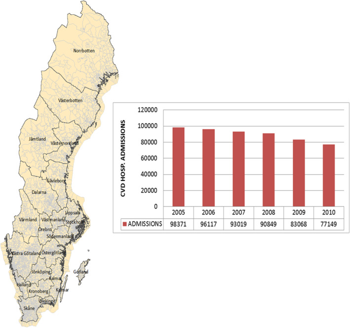
Sweden Counties (with SAMS) and trends of CVD hospital admissions in Sweden from 2005 to 2010. CVD, cardiovascular disease; SAMS, small area for market statistics.

3.2.2. Emission Data

The emission data (hereinafter used interchangeably with “air pollution”) used in this research was based on the Swedish Environmental Emissions Data (SMED) and consists of particulate matter (PM10 and PM2.5), Black Carbon, Sulfur Oxides and Carbon monoxide emission records across Sweden, in a 1 km by 1 km grid resolution for the period 2005 to 2010. The details for the calculation of the 1 km by 1 km grid estimates and the validation of these estimates were discussed by Gidhagen, Johansson, and Omstedt (2009). The SMED consortium uses this very emission inventories for the report of greenhouse gases to the European Commission, under the Climate Convention obligation (Gidhagen, Johansson, & Omstedt, 2009; Gidhagen, Omstedt, et al., 2013). The data was generated by SMED as annual averages from eight sectors of the power supply, industrial processes, product usage, transportation, work machines, agriculture, waste and sewerage, and international aviation and shipping (SMED, 2016). As such, this emission data was used as a proxy for exposure. The same data has previously been used, at the urban level, by Stockfelt et al. (2017) in their study of air pollution and CVD in the city of Gothenburg, Sweden.

3.2.3. Neighborhood Deprivation Index

NDI is a summary measure used to characterize neighborhood‐level deprivation. Deprivation indicators that have been used in previous studies (Crump et al., 2011; Lofors and Sundquist, 2007; Winkleby et al., 2007) were identified to characterize neighborhoods; principal component analysis was then used to generate the SAMS specific z‐score (first principal component) indicative of NDI. Four variables were selected for persons aged 25–64 years. These four were low educational status (<10 years of formal education); unemployment (not employed, excluding full‐time students, those completing compulsory military service, and early retirees); social welfare recipient (receiving social welfare support); and low income (income from all sources, defined as less than 50% of individual median income.

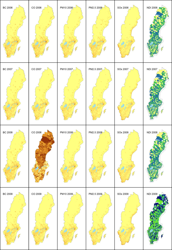
Emission variables (BC, CO, PM10, PM2.5, and SOx) and NDI have been visualized through Figure 2. For brevity, only the first (2005) and the last (2010) years have been visualized here. The visualizations for the remaining years can be found in Appendix A.

Figure 2.

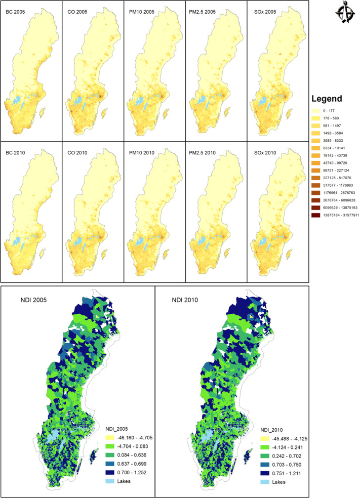
Emission variables and NDI for 2005 and 2010. NDI, Neighborhood Deprivation Index.

The NDI ranges are: <−1 = low deprivation; −1 to 1 = moderate deprivation; >1 = high deprivation (Winkleby et al., 2007).

3.3. Study Methodology

To study the associative spatial heterogeneity of air pollutants and CVD morbidity, we used a Poisson framework, in a progressive way, to model the associative relationships between ambient air pollution and CVD admissions in Sweden while accounting for neighborhood deprivation. Poisson was chosen because the observed CVD admissions were recorded as counts the local expected number was low.

Global Poisson model (GPM) was applied first to recognize the relations of individual pollutants with CVD, in addition to understanding the significance of these relations at the global level. The existence of spatial correlation in data results in biased estimates of the global models (Anselin, 1988; Anselin & Rey, 1991). Given that the GPM does not account for spatial effects in the observed CVD, a spatial lag term was introduced to address the influence of neighborhood values on the observed CVD values to the GPM, leading to the spatial auto‐regression Poisson (SAR‐Poisson) model. This was important as CVD cases in a region are also influenced by the underlying socio‐economic, demographic and environmental factors (Poulter, 1999), which are seldom random in space. However, SAR‐Poisson, being a global model, does not handle local spatial heterogeneity in the obtained associations.

Regression models that allow for geographical weighting are better suited for handling spatial heterogeneity (Nakaya, 2015). We thus employed Geographically Weighted Poisson Regression (GWPR) model that allows for the establishment of coefficient terms and all other regression parameters for each spatial unit (8,419 units for our case).

3.4. Statistical Methods

We investigated the associations between annual ambient air pollution exposures (PM10, PM2.5, BC, SOx, and CO) from the eight sectors (power supply, industrial processes, product usage, transportation, work machines, agriculture, waste and sewerage, and international aviation and shipping), NDI and CVD admission count. Let $y_i$ be the CVD admission count for a particular SAMS $\left(i\right)$. Denote the five ambient air pollution determinants, and NDI as $x_{k,i},k=1,2,\dots .,6$. The SAMS specific population is taken as an offset and is denoted by $N_i$. The conventional GPM can then be specified by Equation 1.

$$y_i\sim \text{Poisson}\left[N_i\text{exp}\left({\displaystyle \sum _k{\beta }_k{x}_{k,i}}\right)\right].$$ (1)

To model for the possible existence of spatial dependence in the observed CVD admissions, SAR‐Poisson model was derived from the original GPM in Equation 1 by adding a spatial lag term, $\rho \left(W_i{y}_i\right)$, shown in Equation 2.

$$y_i\sim \text{Poisson}\left[N_i\text{exp}\left(\rho \left(W_i{y}_i\right)+{\displaystyle \sum _k{\beta }_k{x}_{k,i}}\right)\right],$$ (2)

where $W_i{y}_i$ is the spatially lagged dependent variable for the weights matrix $W_i$, and $\rho$ is a spatially lagged coefficient. The weight matrix was defined by considering n‐nearest neighbors.

GWPR extends this traditional model by allowing for all parameters to vary with geographical location, defined by SAMS in our study. This introduces a location parameter, ${\mathit{u}}_i=(u_{xi},u_{yi})$, a vector containing the two‐dimensional coordinates describing the location of the particular SAMS (centroid coordinates). The Poisson model in Equation 1 can be rewritten as Equation 3.

$$O_i\sim \text{Poisson}\left[N_i\text{exp}\left({\displaystyle \sum _k{\beta }_k\left({\mathit{u}}_i\right)x_{k,i}}\right)\right].$$ (3)

The regression coefficients $\beta$s in Equation 3 are calculated for every SAMS $\left(i\right)$, making them spatially varying. This makes GWPR a local spatial regression model allowing for geographically varying parameters. In our study, there were a total of 8,419 estimated coefficients corresponding to the 8,419 SAMS used.

The geographical weighting in GWPR is such that a kernel window is placed around every SAMS, and the $\beta$s are computed using all the data contained within the kernel window, allowing for neighborhood data to contribute to the value of $\beta$ at that specific SAMS. A bi‐square adaptive weighting kernel, defined by Equation 4, was used for our study.

$$w_{ik}={\left[1-{\left(\frac{d_{ik}}{h}\right)}^2\right]}^2\text{if}{d}_{ik}\le h;\text{otherwise}0,$$ (4)

where $d_{ik}$ is the distance between SAMS $\left(i\right)$ and the nearby SAMS $\left(k\right)$. Observations closer to SAMS $\left(i\right)$ would carry more weights and have greater impacts on parameter estimates than those far away, following the first law of geography (Tobler, 1970). $h$ is a constant bandwidth defining the neighborhood, and for GWPR. It denotes a value that yields the lowest Akaike Information Criterion (AIC), a metric that deals with the trade‐off between the goodness of fit of the model and model simplicity. It is defined by Equation 5, through the bandwidth selection procedure (Nakaya et al., 2005).

$$\text{AIC}\left(G\right)=D\left(G\right)+2K\left(G\right),$$ (5)

where D and K denote the deviance and the effective number of parameters in the model with bandwidth G, respectively.

4. Results

To examine the possible determinants the spatial variation of CVD across Sweden and over time, each ambient air pollution variable and NDI were regressed against the SAMS‐specific CVD outcome. Table 1 shows the model estimates for the GPM model combining all the independent variables. Generally, the associations were both positive and negative except for SOx that was positive throughout.

Table 1.

Global Poisson Model Estimates (2005–2010)

	Estimate (2005)	Estimate (2006)	Estimate (2007)	Estimate (2008)	Estimate (2009)	Estimate (2010)
(Intercept)	−0.207***  a	−0.2364***	−0.271***	−0.3117***	−0.3911***	−0.4653**
NDI	−0.058***	0.05548***	0.05565***	0.05709***	−0.0618***	−0.06027***
BC	−5.275E−07**	−4.846E−07**	−8.8E−07***	−1.1E−06***	−1.8E−06***	−1.6E−06***
CO	−7.064E−09***	−7.53E−09***	−4.1E−09**	3.56E−09***	3.85E−09*	3.98E−09.
PM10	2.295E−07***	1.559E−07***	2.23E−07***	1.3E−07***	5.28E−08	−3.7E−08
PM2.5	−2.798E−07***	−1.173E−07**	−2.6E−07***	−1.8E−07***	−1E−07.	3.49E−08
SOx	3.19E−08***	1.531E−08*	3.12E−08***	3.82E−08***	4.92E−08***	3.51E−08***

Abbreviation: BC, Black Carbon; CO, Carbon monoxide; NDI, Neighborhood Deprivation Index; PM, particulate matter; SOx, Sulfur oxides.

^aSignificant codes: “***” 0.001; “**” 0.01; “*” 0.05; “.”; 0.1; “ ” 1.

Table 2 shows the SAR‐Poisson model estimates. All the variables generally remained significant throughout the years, consistent with the results from the GPM. However, the introduction of the lag term created some changes in the nature of the associations observed in the overall GPM. For example, PM10 becomes consistently negative while PM2.5 becomes consistently positive. CO and the NDI term retain their mixed associations.

Table 2.

Spatial Autoregressive Global Poisson Model Estimate (2005–2010)

	Estimate (2005)	Estimate (2006)	Estimate (2007)	Estimate (2008)	Estimate (2009)	Estimate (2010)
(Intercept)	−0.3904***	−0.4181***	−0.4546***	−0.4975***	−0.5718***	−0.6523***
Lag	0.01426***	0.01464***	0.01518***	0.01585***	0.01656***	0.01834***
NDI	−0.04152***	0.03937***	0.03987***	0.04134***	−0.04672***	−0.04522***
BC	−3.926E−07**	−2.47E−07.	−6.3E−07***	−8.7E−07***	−1.2E−06***	−1.3E−06***
CO	−5.843E−09***	−3.807E−09**	−3.6E−09*	3.17E−09***	2.02E−09	4.67E−09*
PM10	−3.321E−07***	−2.619E−07***	−3.3E−07***	−4.2E−07***	−5E−07***	−5.8E−07***
PM2.5	4.747E−07***	3.837E−07***	4.92E−07***	5.76E−07***	6.76E−07***	7.67E−07***
SOx	1.156E−08	7.031E−09	8.4E−09	2.2E−08*	2.25E−08*	1.52E−08.

Abbreviation: BC, Black Carbon; CO, Carbon monoxide; NDI, Neighborhood Deprivation Index; PM, particulate matter; SOx, Sulfur oxides.

This unstable nature of the associations could be possibly due to multicollinearity existing within the air pollution and NDI variables as shown by Table 3.

Table 3.

Pearson Correlation Between Participating Variables

		NDI_2005	BC	CO	PM10	PM2.5	SOx
NDI_2005		1	−0.161 a	−0.180 a	−0.119 a	−0.062 a	−0.023 b
BC		–	1	0.822 a	0.674 a	0.629 a	0.480 a
CO		–	–	1	0.845 a	0.789 a	0.463 a
PM10		–	–	–	1	0.983 a	0.662 a
PM2.5		–	–	–	–	1	0.694 a
SOx		–	–	–	–	–	1

		NDI_2006	BC	CO	PM10	PM2.5	SOx
NDI_2006		1	0.153 a	0.178 a	0.131 a	0.037 a	0.025 b
BC		–	1	0.804 a	0.683 a	0.554 a	0.447 a
CO		–	–	1	0.851 a	0.698 a	0.429 a
PM10		–	–	–	1	0.943 a	0.655 a
PM2.5		–	–	–	–	1	0.708 a
SOx		–	–	–	–	–	1

		NDI_2007	BC	CO	PM10	PM2.5	SOx
NDI_2007		1	0.147 a	0.173 a	0.126 a	0.071 a	0.020
BC		–	1	0.809 a	0.675 a	0.633 a	0.441 a
CO		–	–	1	0.851 a	0.795 a	0.447 a
PM10		–	–	–	1	0.979 a	0.655 a
PM2.5		–	–	–	–	1	0.696 a
SOx		–	–	–	–	–	1

		NDI_2008	BC	CO	PM10	PM2.5	SOx
NDI_2008		1	0.128 a	−0.016	0.104 a	0.053 a	0.008
BC		–	1	−0.050 a	0.652 a	0.625 a	0.430 a
CO		–	–	1	−0.045 a	−0.037 a	−0.009
PM10		–	–	–	1	0.982 a	0.683 a
PM2.5		–	–	–	–	1	0.716 a
SOx		–	–	–	–	–	1

		NDI_2009	BC	CO	PM10	PM2.5	SOx
NDI_2009		1	−0.142 a	−0.149 a	−0.094 a	−0.050 a	−0.015
BC		–	1	0.812 a	0.657 a	0.619 a	0.471 a
CO		–	–	1	0.874 a	0.832 a	0.561 a
PM10		–	–	–	1	0.985 a	0.742 a
PM2.5		–	–	–	–	1	0.772 a
SOx		–	–	–	–	–	1

		NDI_2010	BC	CO	PM10	PM2.5	SOx
NDI_2010		1	−0.115 a	−0.123 a	−0.080 a	−0.040 a	−0.010
BC		–	1	0.763 a	0.628 a	0.610 a	0.459 a
CO		–	–	1	0.905 a	0.881 a	0.654 a
PM10		–	–	–	1	0.988 a	0.785 a
PM2.5		–	–	–	–	1	0.806 a
SOx		–	–	–	–	–	1

Abbreviation: BC, Black Carbon; CO, Carbon monoxide; NDI, Neighborhood Deprivation Index; PM, particulate matter; SOx, Sulfur oxides.

^aCorrelation is significant at the 0.01 level (2‐tailed).

^bCorrelation is significant at the 0.05 level (2‐tailed).

Table 3 shows that the correlation between NDI and most air pollutants is low and mixed (both positive and negative). Negative correlations were observed for 2005, 2009, and 2010 while positive correlations were observed for 2006, 2007, and 2008 (except for CO). As expected, the air pollutants exhibited high correlations between each other with the highest being between PM10 and PM2.5. The lowest correlation was consistently exhibited between BC and CO.

Additionally, by computing for the Variation Inflation Factor (VIF) statistic for the five variables, values ranging from 2 to 20 were obtained. Ideally, these values should be less than 5; values between 5 and 10 indicate moderate multicollinearity while values above 10 indicate extreme multicollinearity (Alves et al., 2016). It thus showed that we were dealing with a substantial amount of multicollinearity.

Being a local regression model, GPWR accounts for spatial heterogeneity and is robust against multicollinearity (Fotheringham & Oshan, 2016). Figure 3 shows the performance of the three models: the GPM, the SAR‐Poisson model and the GWPR model. The lower the AIC value, the better the performance. It shows that GWPR is the best model as it consistently has the lowest AIC values, followed by SAR‐Poisson, and GPM is the worst as it has the highest AIC values throughout the study period.

Figure 3.

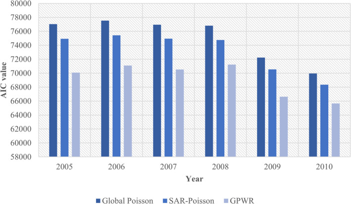
Model performance by akaike information criterion (AIC) for the 3 models.

Table 4 shows the summary of parameter estimates as obtained from the GWPR model. They are described by the minimum, lower quartile, median, upper quartile, and the maximum. Given that the parameter values were not standardized in the global models, the intercept is the only comparable parameter between the global and these local estimates. We note that the median intercept coefficient estimates for both models (GWPR and overall GPM) were relatively similar, for all the years. Additionally, some parameter estimates range from negative to positive over the study area, exhibiting a wider dynamic range compared to the averaged values reported by GPM.

Table 4.

Summary Statistics for Varying (Local) Coefficients From the GWPR Model

Coefficients	Minimum of coefficients	Lower quartile of coefficients	Median of coefficients	Upper quartile of coefficients	Maximum of coefficients
2005 Intercept	0.898	1.316	1.438	1.572	1.841
NDI_2005	−0.750	−0.513	−0.429	−0.283	−0.093
BC	−2.565	−0.213	−0.016	0.217	1.490
CO	−1.874	−0.123	0.074	0.371	1.629
PM10	−6.988	−0.976	−0.181	0.508	3.759
PM2.5	−2.857	−0.339	0.152	0.784	4.847
SOx	−5.605	−0.156	−0.039	0.038	6.241
2006 Intercept	0.873	1.302	1.403	1.551	1.793
NDI_2006	0.090	0.268	0.440	0.509	0.783
BC	−3.038	−0.313	−0.057	0.174	1.558
CO	−1.888	−0.043	0.144	0.443	1.543
PM10	−4.268	−0.893	−0.109	0.446	4.085
PM2.5	−1.559	−0.210	0.075	0.577	2.569
SOx	−5.365	−0.151	−0.027	0.090	6.384
2007 Intercept	0.813	1.263	1.371	1.531	1.759
NDI_2007	0.092	0.257	0.419	0.499	0.776
BC	−2.534	−0.209	−0.001	0.231	1.870
CO	−2.005	−0.078	0.113	0.366	1.321
PM10	−5.239	−0.895	−0.227	0.375	4.561
PM2.5	−2.553	−0.314	0.158	0.539	4.691
SOx	−5.113	−0.126	−0.021	0.062	8.773
2008 Intercept	0.715	1.243	1.357	1.492	1.733
NDI_2008	0.097	0.257	0.407	0.486	0.782
BC	−3.846	−0.128	0.100	0.333	1.404
CO	−0.499	−0.143	−0.032	0.023	0.228
PM10	−5.158	−0.691	−0.185	0.509	7.446
PM2.5	−3.548	−0.443	0.151	0.678	5.132
SOx	−5.250	−0.196	−0.048	0.031	9.307
2009 Intercept	0.654	1.131	1.250	1.414	1.738
NDI_2009	−0.784	−0.463	−0.395	−0.272	−0.098
BC	−3.313	−0.280	−0.051	0.189	1.976
CO	−2.149	−0.002	0.188	0.408	1.575
PM10	−5.582	−1.368	−0.351	0.391	8.087
PM2.5	−2.951	−0.228	0.314	0.879	5.191
SOx	−5.787	−0.128	−0.018	0.128	10.021
2010 Intercept	0.520	1.036	1.185	1.338	1.764
NDI_2010	−0.842	−0.450	−0.400	−0.288	−0.100
BC	−2.314	−0.283	−0.092	0.061	2.092
CO	−2.116	−0.006	0.228	0.544	1.563
PM10	−7.036	−1.370	−0.480	0.392	4.762
PM2.5	−5.386	−0.188	0.401	0.973	6.651
SOx	−4.454	−0.190	−0.034	0.122	12.116

Abbreviation: BC, Black Carbon; CO, Carbon monoxide; NDI, Neighborhood Deprivation Index; PM, particulate matter; SOx, Sulfur oxides.

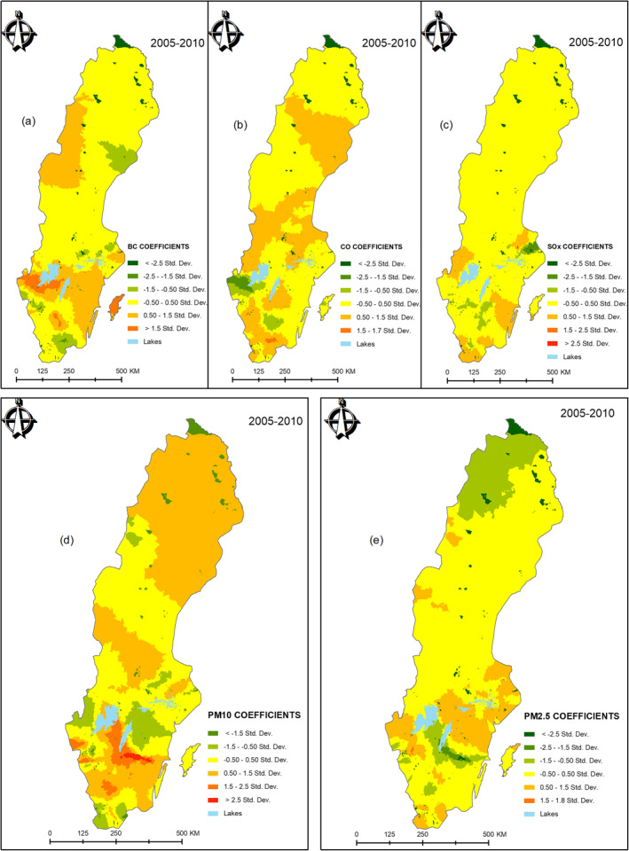
The spatial variation of the associations between CVD and the five air pollution variables (BC, CO, PM10, PM2.5, and SOx) were visualized by maps. The mean spatial variations of the coefficients of all the five air pollutants are given by Figure 4. This was obtained by averaging SAMS‐specific coefficients for individual pollutants, over the 6 years. Labels (a–e) in Figure 4 was used to distinguish the spatial coefficient variations for BC, CO, SOx, PM10, and PM2.5, respectively. By averaging, areas of particularly persistent high associations were highlighted. For example, BC (a) shows a moderately strong association in Gotland (an island in the southeast), across mid‐lower‐western regions and mid‐upper‐western regions of Sweden. Weaker associations for BC are observed mainly in the northern parts of Sweden. PM10 (d) is the most pronounced with strongest associations in the mid‐lower parts of Sweden and persistently moderate to strong associations in the North. CO (b) and SOx (c) show generally moderate associations while PM2.5 (e) shows generally low associations with CVD, across Sweden. The upper northern part particularly shows lower associations with PM2.5 over the 6‐year study period.

Figure 4.

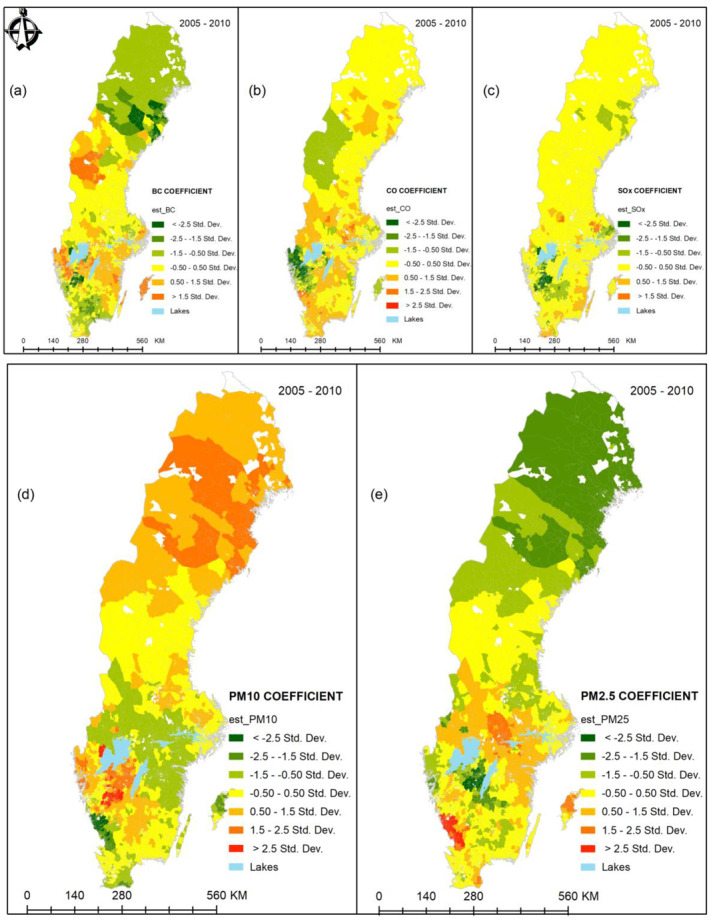
Combined spatial variations (2005–2010) in (a) BC, (b) CO, (c) SOx, (d) PM10, and (e) PM2.5. BC, Black Carbon; CO, Carbon monoxide; NDI, Neighborhood Deprivation Index; PM, particulate matter; SOx, Sulfur oxides.

5. Discussion

This study employed a spatial perspective with emphasis on spatial non‐stationarity to assess the association between ambient air pollution variables (BC, CO, PM10, PM2.5, and SOx) and CVD admissions while accounting for neighborhood deprivation in Sweden from 2005 to 2010. Neighborhood deprivation in the form of the established index, NDI, was used to account for the underlying socio‐economic variables mainly because it has been shown to independently predict heart disease morbidity. The results of our analysis also showed that NDI had a mixed but significant association with CVD in Sweden, as indicated by the results of the global Poisson models. The significant association was consistent with the results obtained by previous studies in Britain (Lawlor et al., 2005) and Sweden (Kawakami et al., 2011; Sundquist, Winkleby, et al., 2004; Winkleby et al., 2007). The mixed nature of the association could point to the inability of the global model to evaluate the associations correctly, given their spatial heterogeneity.

The GWPR model as an effective tool to evaluate these non‐stationary relations was used to compute the spatially varying regression parameter estimates across Sweden. GWPR assumes a Poisson distribution to model count‐based outcomes and is hence statistically more appropriate than conventional regression models based on Gaussian distribution like conditional and simultaneous autoregressive models (V. Y.‐J. Chen et al., 2010). Through the Akaike Information Criterion (AIC) statistic, Figure 3 shows that GWPR was the best model fit against global Poisson models as measured by the lowest AIC value. It was followed by SAR‐Poisson, and global Poisson model was the worst of the models. To examine how GWPR successfully captured the spatially non‐stationary variations in the coefficient parameters, Table 4 was examined. Here, some estimated coefficients range from negative to positive over the study area. This indicates how GPWR was able to capture the spatial non‐stationarity, and how the global models (in Tables 1 and 2) can be misleading by assuming constant association coefficients across the study area.

We argue that traffic‐related PM10 could be responsible for the persistent strong associations with CVD in the middle‐south and southwest of Sweden (Figure 4). This position is consistent with the results of Segersson et al. (2017) who contended that PM10 and BC are primarily produced by road traffic through both wear particles and exhaust. However, the moderately stronger associations of PM10 in the northern part of Sweden were unclear to attribute to any specific source. PM2.5, CO, and BC are known to be mainly produced by residential wood combustion and road traffic sources (Segersson et al., 2017; Stockfelt et al., 2017). We thus speculate that residential wood heating, fuel burning, and road traffic could be largely responsible for the observed spatial patterns between BC, PM10, PM2.5, and CO air pollution and CVD in Figure 4 (visualization of the spatial patterns while not accounting for NDI is provided in Appendix B). On the other hand, SOx is known to be a shipping pollutant due to the high sulfur content of marine fuels (Nikopoulou et al., 2013). Therefore, the patterns observed in SOx associations could be attributed to the numerous navigational routes along the coastline (especially the southern half of Sweden).

It should be emphasized that our interpretation of place‐specific association obtained in this study is more general as pollutants may exhibit associations in places away from their sources. This noncommittal interpretation was called for by Meister et al. (2012) who cautioned about the interpreting place‐specific associations of PM2.5 and health outcomes as large portions of it in cities tend to be transported over long distances.

Our findings, having considered spatial heterogeneity, were consistent with conclusions from previous studies (Alves et al., 2016; Feuillet et al., 2015; Gomes et al., 2017; Z. Li et al., 2013; Lim et al., 2014; Nakaya, 2015; Nakaya et al., 2005) regarding the heterogeneity of relations. From global models, we observed generally weak but highly significant associations between air pollution variables and CVD, evidenced by relatively small coefficient values. These weak and mixed associations were also observed by R. Chen et al. (2017) in China, Stockfelt et al. (2017) and Taj et al. (2017) in their city‐specific studies in Sweden. This could be generally explained by the fact that CVD is multi‐factorial (Poulter, 1999) and influenced by many other lifestyle and socio‐economic determinants, like smoking, hypertension, lack of exercises, to mention but a few, in addition to ambient air pollution. However, they could also be due to the combined effects of overdispersion and multicollinearity in the data (Gomes et al., 2017).

Overdispersion issues are well handled by Global Negative Binomial models (GNB), and would as such be a better alternative (Alves et al., 2016; Z. Li et al., 2013). However, given the spatial nature of the data as evidenced by the significant lag term in the SAR‐Poisson model, we reasoned that the probabilistic mechanisms used by global GNB to handle such overdispersion would overlook its specific local‐scale causes, which was also mentioned by Alves et al. (2016). Moreover, our tests showed that the global GNB results were not very different from the GPM results. Additionally, the unobserved heterogeneity as computed from the density of variance of GNB random effects (Rodríguez, 2019) had the quartile ranges [0.185 (Q1), 0.581 (Q2), and 1.373 (Q3)], meaning that CVD admissions at the lower quantile of the unobserved heterogeneity were 81% lower than expected, CVD admissions at the median were 8% higher and those at the upper quantile were 37% higher than expected. The observed overdispersion was therefore in part due to heterogeneity, which is better handled by local spatial models.

While for the local model, GWNBR is known to better handle overdispersion than GWPR (da Silva & Rodrigues, 2014), applying GWNBR on a section of our data set resulted in banding effects, characterized by homogeneous regions in the resultant coefficient maps. This could be attributed to the bandwidth selection procedure converging at wider bandwidths for GWNBR which shows that GWNBR was not able to handle spatial heterogeneity. This was consistent with results obtained by Gomes et al. (2017). It was thus a split‐decision between better handling of either overdispersion (GWNBR) or heterogeneity (GWPR). Since spatial heterogeneity was our primary goal, GWPR was selected for our analysis.

Multicollinearity between air pollution variables has been highlighted by Stockfelt et al. (2017) as the limitation responsible for few multi‐pollution studies like our own. However, in an elaborate study of GWR, Fotheringham and Oshan (2016) illustrated that GWR is robust even under extreme multicollinearity and produces reliable results.

Finally, whereas this study achieved what it set out to do, the authors are aware that this being an ecological study, there is a need to acknowledge ecological bias. Given that all data (CVD and air pollution) had to be aggregated to SAMS level (underlying population was available at this level), the obtained associations cannot reflect the would‐be associations at the individual level. Also, the data used is of 10 years ago. To this end, air quality and social characteristics may change over time. However, the biological effects of these air pollution exposures are likely to remain the same over time and therefore, we believe that our obtained results are therefore still very relevant.

6. Conclusions

The primary contribution of this study is the global as well as local analyses of the association between several established air pollutants and CVD in Sweden, on a nationwide basis while accounting for socio‐economic factors through an established neighborhood deprivation index. It has successfully demonstrated that multi‐pollutant associations with CVD are not homogenous across Sweden and is, to the best of our knowledge, the first nationwide study that spatially analyses multi‐pollutant data and CVD with a particular focus on spatial non‐stationarity. In this 6‐year study of CVD admission counts and ambient air pollution, we found generally weak but statistically significant global associations between main particulate matter pollutants and CVD admissions. More importantly, using GWPR, we found these associations to be non‐homogeneous but varied across space. Generally, more dynamism in the observed patterns was associated with southern parts of Sweden than with the northern regions. These results are, despite certain limitations, useful because they indicate that health policies targeting air pollution and CVD preventive and management efforts in Sweden may be defined at local levels rather than at a global (national–in this case) level. Moreover, with areas of persistent high associations between air pollution and CVD identified, more focused studies could be conducted in these areas to learn more about the drivers of such associations to better inform future healthcare policy and intervention efforts.

Conflict of Interest

The authors declare no conflicts of interest relevant to this study.

Appendix A.

A.1.

The spatial patterns for most air pollutants and NDI are visually similar for the studied years, apart from CO for 2008 (see Figure A1). The reason for the different patterns for CO in 2008 is not known but relates to the data provided.

Figure A1.

Variation of air pollution and NDI variables (2006–2009).

Appendix B.

B.1.

In Figure B1, the spatial patterns of the association between CVD and the selected air pollutants with accounting for NDI seem visually comparable to those obtained in Figure 4. Accounting for NDI works to accentuate the obtained associations.

Figure B1.

Combined Spatial Variations (2005–2010) in (a) BC, (b) CO, (c) SOx, (d) PM10, and (e) PM2.5 – without NDI.

Aturinde, A. , Farnaghi, M. , Pilesjö, P. , Sundquist, K. , & Mansourian, A. (2021). Spatial analysis of ambient air pollution and cardiovascular disease (CVD) hospitalization across Sweden. GeoHealth, 5, e2020GH000323. 10.1029/2020GH000323

Data Availability Statement

The data sets generated and/or analyzed during the current study are not publicly available due to integrity and legal reasons but are available from the corresponding author on reasonable request.

References

- Alexeeff, S. E. , Roy, A. , Shan, J. , Liu, X. , Messier, K. , Apte, J. S. , et al. (2018). High‐resolution mapping of traffic related air pollution with Google street view cars and incidence of cardiovascular events within neighborhoods in Oakland, CA. Environmental Health, 17(1), 38. 10.1186/s12940-018-0382-1 [DOI] [PMC free article] [PubMed] [Google Scholar]
- Alves, A. T. J. , Nobre, F. F. , & Waller, L. A. (2016). Exploring spatial patterns in the associations between local AIDS incidence and socioeconomic and demographic variables in the state of Rio de Janeiro, Brazil. Spatial and Spatio‐temporal Epidemiology, 17, 85–93. 10.1016/j.sste.2016.04.008 [DOI] [PubMed] [Google Scholar]
- Anselin, L. (1988). Spatial econometrics: Methods and models. Kluwer Academic Publishers. [Google Scholar]
- Anselin, L. , & Rey, S. (1991). Properties of tests for spatial dependence in linear regression models. Geographical Analysis, 23(2), 112–131. [Google Scholar]
- Atkinson, R. W. , Carey, I. M. , Kent, A. J. , van Staa, T. P. , Anderson, H. R. , & Cook, D. G. (2013). Long‐term exposure to outdoor air pollution and incidence of cardiovascular diseases. Epidemiology, 24, 44–53. 10.1097/ede.0b013e318276ccb8 [DOI] [PubMed] [Google Scholar]
- Beelen, R. , Hoek, G. , van den Brandt, P. A. , Goldbohm, R. A. , Fischer, P. , Schouten, L. J. , et al. (2008). Long‐term effects of traffic‐related air pollution on mortality in a Dutch cohort (NLCS‐AIR study). Environmental Health Perspectives, 116(2), 196–202. 10.1289/ehp.10767 [DOI] [PMC free article] [PubMed] [Google Scholar]
- Bell, M. L. , Ebisu, K. , Peng, R. D. , Walker, J. , Samet, J. M. , Zeger, S. L. , & Dominici, F. (2008). Seasonal and Regional Short‐term effects of fine particles on hospital admissions in 202 US Counties, 1999–2005. American Journal of Epidemiology, 168(11), 1301–1310. 10.1093/aje/kwn252 [DOI] [PMC free article] [PubMed] [Google Scholar]
- Blangiardo, M. , Finazzi, F. , & Cameletti, M. (2016). Two‐stage Bayesian model to evaluate the effect of air pollution on chronic respiratory diseases using drug prescriptions. Spatial and Spatio‐temporal Epidemiology, 18, 1–12. 10.1016/j.sste.2016.03.001 [DOI] [PubMed] [Google Scholar]
- Brook, R. D. , Franklin, B. , Cascio, W. , Hong, Y. , Howard, G. , Lipsett, M. , et al. (2004). Air pollution and cardiovascular disease. Circulation, 109(21), 2655–2671. 10.1161/01.cir.0000128587.30041.c8 [DOI] [PubMed] [Google Scholar]
- Brooke, H. L. , Talbäck, M. , Hörnblad, J. , Johansson, L. A. , Ludvigsson, J. F. , Druid, H. , et al. (2017). The Swedish cause of death register. European Journal of Epidemiology, 32(9), 765–773. 10.1007/s10654-017-0316-1 [DOI] [PMC free article] [PubMed] [Google Scholar]
- Burnett, R. , Ma, R. , Jerrett, M. , Goldberg, M. S. , Cakmak, S. , Pope, C. A., III , & Krewski, D. (2001). The spatial association between community air pollution and mortality: A new method of analyzing correlated geographic cohort data. Environmental Health Perspectives, 109, 375–380. 10.2307/3434784 [DOI] [PMC free article] [PubMed] [Google Scholar]
- Chen, R. , Yin, P. , Meng, X. , Liu, C. , Wang, L. , Xu, X. , et al. (2017). Fine particulate air pollution and daily mortality. A nationwide analysis in 272 Chinese cities. American Journal of Respiratory and Critical Care Medicine, 196(1), 73–81. 10.1164/rccm.201609-1862oc [DOI] [PubMed] [Google Scholar]
- Chen, V. Y.‐J. , Wu, P.‐C. , Yang, T.‐C. , & Su, H.‐J. (2010). Examining non‐stationary effects of social determinants on cardiovascular mortality after cold surges in Taiwan. Science of the Total Environment, 408(9), 2042–2049. 10.1016/j.scitotenv.2009.11.044 [DOI] [PubMed] [Google Scholar]
- Cohen, A. J. , Brauer, M. , Burnett, R. , Anderson, H. R. , Frostad, J. , Estep, K. , et al. (2017). Estimates and 25‐year trends of the global burden of disease attributable to ambient air pollution: An analysis of data from the global burden of diseases study 2015. The Lancet, 389(10082), 1907–1918. 10.1016/s0140-6736(17)30505-6 [DOI] [PMC free article] [PubMed] [Google Scholar]
- Crump, C. , Sundquist, K. , Sundquist, J. , & Winkleby, M. A. (2011). Neighborhood deprivation and psychiatric medication prescription: A Swedish national multilevel study. Annals of Epidemiology, 21(4), 231–237. 10.1016/j.annepidem.2011.01.005 [DOI] [PMC free article] [PubMed] [Google Scholar]
- da Silva, A. R. , & Rodrigues, T. C. V. (2014). Geographically weighted negative binomial regression—incorporating overdispersion. Statistics and Computing, 24(5), 769–783. [Google Scholar]
- Dominici, F. , Peng, R. D. , Bell, M. L. , Pham, L. , McDermott, A. , Zeger, S. L. , & Samet, J. M. (2006). Fine particulate air pollution and hospital admission for cardiovascular and respiratory diseases. Journal of the American Medical Association, 295(10), 1127–1134. 10.1001/jama.295.10.1127 [DOI] [PMC free article] [PubMed] [Google Scholar]
- Feuillet, T. , Charreire, H. , Menai, M. , Salze, P. , Simon, C. , Dugas, J. , et al. (2015). Spatial heterogeneity of the relationships between environmental characteristics and active commuting: Toward a locally varying social ecological model. International Journal of Health Geographics, 14(1), 12. 10.1186/s12942-015-0002-z [DOI] [PMC free article] [PubMed] [Google Scholar]
- Fotheringham, A. S. , Brunsdon, C. , & Charlton, M. (2002). Geographically weighted regression: The analysis of spatially varying relationships. John Wiley & Sons, Limited. [Google Scholar]
- Fotheringham, A. S. , Crespo, R. , & Yao, J. (2015). Geographical and temporal weighted regression (GTWR). Geographical Analysis, 47(4), 431–452. 10.1111/gean.12071 [DOI] [Google Scholar]
- Fotheringham, A. S. , & Oshan, T. M. (2016). Geographically weighted regression and multicollinearity: Dispelling the myth. Journal of Geographical Systems, 18(4), 303–329. 10.1007/s10109-016-0239-5 [DOI] [Google Scholar]
- Gidhagen, L. , Johansson, H. , & Omstedt, G. (2009). SIMAIR—Evaluation tool for meeting the EU directive on air pollution limits. Atmospheric Environment, 43(5), 1029–1036. 10.1016/j.atmosenv.2008.01.056 [DOI] [Google Scholar]
- Gidhagen, L. , Omstedt, G. , Pershagen, G. , Willers, S. , & Bellander, T. (2013). High‐resolution modeling of residential outdoor particulate levels in Sweden. Journal of Exposure Science and Environmental Epidemiology, 23(3), 306–314. 10.1038/jes.2012.122 [DOI] [PubMed] [Google Scholar]
- Gomes, M. J. T. L. , Cunto, F. , & da Silva, A. R. (2017). Geographically weighted negative binomial regression applied to zonal level safety performance models. Accident Analysis & Prevention, 106, 254–261. 10.1016/j.aap.2017.06.011 [DOI] [PubMed] [Google Scholar]
- Grahame, T. J. , & Schlesinger, R. B. (2010). Cardiovascular health and particulate vehicular emissions: A critical evaluation of the evidence. Air Quality, Atmosphere, & Health, 3(1), 3–27. 10.1007/s11869-009-0047-x [DOI] [PMC free article] [PubMed] [Google Scholar]
- Hadley, M. B. , Baumgartner, J. , & Vedanthan, R. (2018). Developing a clinical approach to air pollution and cardiovascular health. Circulation, 137(7), 725–742. 10.1161/circulationaha.117.030377 [DOI] [PMC free article] [PubMed] [Google Scholar]
- Jerrett, M. , Turner, M. C. , Beckerman, B. S. , Pope, C. A. , van Donkelaar, A. , Martin, R. V. , et al. (2017). Comparing the health effects of ambient particulate matter estimated using ground‐based versus remote sensing exposure estimates. Environmental Health Perspectives, 125(4), 552–559. 10.1289/ehp575 [DOI] [PMC free article] [PubMed] [Google Scholar]
- Kawakami, N. , Li, X. , & Sundquist, K. (2011). Health‐promoting and health‐damaging neighbourhood resources and coronary heart disease: A follow‐up study of 2 165000 people. Journal of Epidemiology & Community Health, 65(10), 866–872. 10.1136/jech.2010.117580 [DOI] [PubMed] [Google Scholar]
- Lawlor, D. A. , Davey Smith, G. , Patel, R. , & Ebrahim, S. (2005). Life‐course socioeconomic position, area deprivation, and coronary heart disease: Findings from the British women's heart and health study. American Journal of Public Health, 95(1), 91–97. 10.2105/ajph.2003.035592 [DOI] [PMC free article] [PubMed] [Google Scholar]
- Le Tertre, A. , Medina, S. , Forsberg, B. , Michelozzi, P. , Boumghar, A. , Vonk, J. M. , et al. (2002). Short‐term effects of particulate air pollution on cardiovascular diseases in eight European cities. Journal of Epidemiology & Community Health, 56(10), 773–779. 10.1136/jech.56.10.773 [DOI] [PMC free article] [PubMed] [Google Scholar]
- Lim, Y.‐R. , Bae, H.‐J. , Lim, Y.‐H. , Yu, S. , Kim, G.‐B. , & Cho, Y.‐S. (2014). Spatial analysis of PM10 and cardiovascular mortality in the Seoul metropolitan area. Environmental Health and Toxicology, 29, e2014005. 10.5620/eht.2014.29.e2014005 [DOI] [PMC free article] [PubMed] [Google Scholar]
- Li, X. , Sundquist, J. , Forsberg, P.‐O. , Sundquist, K. (2020). Association between neighborhood deprivation and heart failure among patients with diabetes mellitus: A 10‐year follow‐up study in Sweden journal of cardiac failure. Journal of cardiac Failure, 26(3), 193–199. 10.1016/j.cardfail.2019.04.017 [DOI] [PMC free article] [PubMed] [Google Scholar]
- Li, Z. , Wang, W. , Liu, P. , Bigham, J. M. , & Ragland, D. R. (2013). Using geographically weighted poisson regression for county‐level crash modeling in California. Safety Science, 58, 89–97. 10.1016/j.ssci.2013.04.005 [DOI] [Google Scholar]
- Lofors, J. , & Sundquist, K. (2007). Low‐linking social capital as a predictor of mental disorders: A cohort study of 4.5 million Swedes. Social Science & Medicine, 64(1), 21–34. [DOI] [PubMed] [Google Scholar]
- Luo, K. , Li, R. , Li, W. , Wang, Z. , Ma, X. , Zhang, R. , et al. (2016). Acute effects of nitrogen dioxide on cardiovascular mortality in Beijing: An exploration of spatial heterogeneity and the district‐specific predictors. Scientific Reports, 6(1), 38328. 10.1038/srep38328 [DOI] [PMC free article] [PubMed] [Google Scholar]
- Meister, K. , Johansson, C. , & Forsberg, B. (2012). Estimated short‐term effects of coarse particles on daily mortality in Stockholm, Sweden. Environmental Health Perspectives, 120(3), 431–436. 10.1289/ehp.1103995 [DOI] [PMC free article] [PubMed] [Google Scholar]
- Nakaya, T. (2015). Geographically weighted generalised linear modelling. In Brunsdon C. & Singleton A. (Eds.), Geocomputation: A practical primer. SAGE. [Google Scholar]
- Nakaya, T. , Fotheringham, A. S. , Brunsdon, C. , & Charlton, M. (2005). Geographically weighted Poisson regression for disease association mapping. Statistics in Medicine, 24(17), 2695–2717. 10.1002/sim.2129 [DOI] [PubMed] [Google Scholar]
- Nikopoulou, Z. , Cullinane, K. , & Jensen, A. (2013). The role of a cap‐and‐trade market in reducing NOx and SOx emissions: Prospects and benefits for ships within the Northern European ECA. Proceedings of the Institution of Mechanical Engineers, Part M: Journal of Engineering for the Maritime Environment, 227(2), 136–154. 10.1177/1475090212459130 [DOI] [Google Scholar]
- Pope, C. A. , Burnett, R. T. , Thurston, G. D. , Thun, M. J. , Calle, E. E. , Krewski, D. , & Godleski, J. J. (2004). Cardiovascular mortality and long‐term exposure to particulate air pollution. Circulation, 109, 71–77. 10.1161/01.cir.0000108927.80044.7f [DOI] [PubMed] [Google Scholar]
- Poulter, N. (1999). Coronary heart disease is a multifactorial disease. American Journal of Hypertension, 12(4), 92–95. 10.1016/s0895-7061(99)00163-6 [DOI] [PubMed] [Google Scholar]
- Qiu, H. , Sun, S. , Tsang, H. , Wong, C.‐M. , Lee, R. S.‐Y. , Schooling, C. M. , & Tian, L. (2017). Fine particulate matter exposure and incidence of stroke. Neurology, 88(18), 1709–1717. 10.1212/wnl.0000000000003903 [DOI] [PubMed] [Google Scholar]
- Rodríguez, G. (2019). Models for over‐dispersed count data (Vol. 2019). Princeton University. [Google Scholar]
- Segersson, D. , Eneroth, K. , Gidhagen, L. , Johansson, C. , Omstedt, G. , Nylén, A. E. , & Forsberg, B. (2017). Health Impact of PM10, PM2.5 and black carbon exposure due to different source sectors in Stockholm, Gothenburg and Umea, Sweden. International Journal of Environmental Research and Public Health, 14(7), 742. 10.3390/ijerph14070742 [DOI] [PMC free article] [PubMed] [Google Scholar]
- SMED . (2016). Description of methods and quality of spatially distributed emissions to air during 2016 (Contract no 309 1235). SMED. (in Swedish, original title: Metod‐och kvalitetsbeskrivning för geografiskt fördelade emissioner till luft under 2016). [Google Scholar]
- Stockfelt, L. , Andersson, E. M. , Molnár, P. , Gidhagen, L. , Segersson, D. , Rosengren, A. , et al. (2017). Long‐term effects of total and source‐specific particulate air pollution on incident cardiovascular disease in Gothenburg, Sweden. Environmental Research, 158, 61–71. 10.1016/j.envres.2017.05.036 [DOI] [PubMed] [Google Scholar]
- Sundquist, K. , Malmström, M. , & Johansson, S. (2004a). Neighbourhood deprivation and incidence of coronary heart disease: A multilevel study of 2.6 million women and men in Sweden. Journal of Epidemiology & Community Health, 58(1), 71–77. 10.1136/jech.58.1.71 [DOI] [PMC free article] [PubMed] [Google Scholar]
- Sundquist, K. , Winkleby, M. , Ahlén, H. , & Johansson, S.‐E. (2004b). Neighborhood socioeconomic environment and incidence of coronary heart disease: A follow‐up study of 25,319 women and men in Sweden. American Journal of Epidemiology, 159(7), 655–662. 10.1093/aje/kwh096 [DOI] [PubMed] [Google Scholar]
- Sundquist, K. , & Yang, M. (2007). Linking social capital and self‐rated health: A multilevel analysis of 11,175 men and women in Sweden. Health & Place, 13(2), 324–334. 10.1016/j.healthplace.2006.02.002 [DOI] [PubMed] [Google Scholar]
- Sun, Q. , Hong, X. , & Wold, L. E. (2010). Cardiovascular effects of ambient particulate air pollution exposure. Circulation, 121(25), 2755–2765. 10.1161/circulationaha.109.893461 [DOI] [PMC free article] [PubMed] [Google Scholar]
- Sunyer, J. , Ballester, F. , Tertre, A. L. , Atkinson, R. , Ayres, J. G. , Forastiere, F. , et al. (2003). The association of daily sulfur dioxide air pollution levels with hospital admissions for cardiovascular diseases in Europe (The Aphea‐II study). European Heart Journal, 24(8), 752–760. 10.1016/s0195-668x(02)00808-4 [DOI] [PubMed] [Google Scholar]
- Taj, T. , Malmqvist, E. , Stroh, E. , Oudin Åström, D. , Jakobsson, K. , & Oudin, A. (2017). Short‐term associations between air pollution concentrations and respiratory health‐comparing primary health care visits, hospital admissions, and emergency department visits in a multi‐municipality study. International Journal of Environmental Research and Public Health, 14(6), 587. 10.3390/ijerph14060587 [DOI] [PMC free article] [PubMed] [Google Scholar]
- Thurston, G. D. , & Newman, J. D. (2018). Walking to a pathway for cardiovascular effects of air pollution. The Lancet, 391(10118), 291–292. 10.1016/s0140-6736(17)33078-7 [DOI] [PMC free article] [PubMed] [Google Scholar]
- Tobler, W. R. (1970). A computer movie simulating urban growth in the Detroit region. Economic Geography, 46, 234–240. 10.2307/143141 [DOI] [Google Scholar]
- Vidale, S. , & Campana, C. (2018). Ambient air pollution and cardiovascular diseases: From bench to bedside. European Journal of Preventive Cardiology, 25(8), 818–825. 10.1177/2047487318766638 [DOI] [PubMed] [Google Scholar]
- WHO . (2019). Cardiovascular disease. World Health Organisation. Retrieved from http://www.who.int/cardiovascular_diseases/en/ [Google Scholar]
- Wilkins, E. , Wilson, L. , Wickramasinghe, K. , Bhatnagar, P. , Rayner, M. , & Townsend, N. (2017). European cardiovascular disease statistics 2017. European Heart Network. [Google Scholar]
- Winkleby, M. , Sundquist, K. , & Cubbin, C. (2007). Inequities in CHD incidence and case fatality by neighborhood deprivation. American Journal of Preventive Medicine, 32(2), 97–106. 10.1016/j.amepre.2006.10.002 [DOI] [PMC free article] [PubMed] [Google Scholar]
- Zhang, L.‐W. , Chen, X. , Xue, X.‐D. , Sun, M. , Han, B. , Li, C.‐P. , et al. (2014). Long‐term exposure to high particulate matter pollution and cardiovascular mortality: A 12‐year cohort study in four cities in northern China. Environment International, 62, 41–47. 10.1016/j.envint.2013.09.012 [DOI] [PubMed] [Google Scholar]
Associated Data
This section collects any data citations, data availability statements, or supplementary materials included in this article.