Automated Method for Generating the Arterial Input Function on Perfusion-Weighted MR Imaging: Validation in Patients with Stroke

Abstract

BACKGROUND AND PURPOSE: The choice of arterial input function (AIF) can have a profound effect on the blood flow maps generated on perfusion-weighted MR imaging (PWI). Automation of this process could substantially reduce operator dependency, increase consistency, and accelerate PWI analysis. We created an automated AIF identification program (auto-AIF) and validated its performance against conventional manual methods.

METHODS: We compared the auto-AIF against manually derived AIFs from multisection PWIs of 22 patients with stroke. Time to peak, curve width, curve height, and voxel location determined with both techniques were compared. The time to maximum of the tissue residue function (Tmax) and cerebral blood flow (CBF) were computed on a per-pixel basis for each AIF. Spatial patterns of 528 map pairs were compared by computing Pearson correlation coefficients between maps generated with each method.

RESULTS: All auto-AIF–derived PWI map parameters, including bolus peak, width, and height, were consistently superior to manually derived ones. Reproducibility of the auto-AIF–based Tmax maps was excellent (r = 1.0). Paired Tmax maps and CBF maps from both techniques were well correlated (r = 0.82). Time to identify the AIF was significantly shorter with the auto-AIF method than with the manual technique (mean difference, 72 seconds; 95% confidence interval: 54, 89 seconds).

CONCLUSION: An automated program that identifies the AIF is feasible and can create reliably reproducible and accurate Tmax and CBF maps. Automation of this process could reduce PWI analysis time and increase consistency and may allow for more effective use of PWI in the evaluation of acute stroke.

Perfusion-weighted MR imaging (PWI) was developed in the late 1980s to study disorders of blood flow (1–8). In dynamic susceptibility contrast imaging, paramagnetic contrast agent passes through the vessels, dephasing protons and altering T2* relaxation in the surrounding tissues proportional to the amount of perfusion. By measuring the corresponding changes in the signal intensity, rapid imaging methods, such as echo-planar imaging, can be used to track a bolus of contrast agent through the entire brain and calculate a time–signal intensity curve for each tissue voxel (9–12). The concentration of the tracer is approximately proportional to the change in the relaxation rate, which in turn is a nonlinear function of the change in signal intensity (13). However, quantification of clinically important parameters, such as mean transit time, time to the maximum of the tissue residual function (Tmax), and cerebral blood flow (CBF), is computationally intensive and requires rather complex analysis.

Ostergaard et al (14, 15) and Wirestam et al (16) reported that it is possible to determine relative CBF accurately by means of mathematical deconvolution of a tissue concentration curve with the arterial input function (AIF) reflecting the concentration of contrast agent entering the region of interest. However, quantitative PWI is difficult and prone to errors. The deconvolution method assumes that the AIF into each tissue voxel is known, when in fact most AIFs are approximated by measuring the AIF from the major cerebral arteries to minimize the error from partial-volume effects. Although estimation of AIF takes care of the delay and spread of the bolus from the site of injection to the site of measurement, any delays and dispersion of the bolus from the site of AIF to the region of interest can introduce an error (17). Choosing the AIF close to the tissue of interest could minimize this error; however, this may not be possible in cases with stenosis or occlusion, in which the AIF from the contralateral side should be used. In addition, for such cases, extra bolus dispersion occurs when an ipsilateral AIF is used instead of a contralateral one (18). Also, PWI lesion volumes determined with an AIF from the contralateral middle cerebral artery (MCA) are better associated with follow-up lesion volume than those determined with an AIF from the ipsilateral MCA (19). Hence, quantifying dynamic susceptibility contrast imaging is often unreliable and in turn complicates data analysis (20).

The choice of AIF is critical for accurate generation of CBF maps. Several groups have reported differences in bolus shape depending on the site chosen (18, 21). Small changes to the AIF location can have a profound effect on the maps generated. Delays and dispersion of the bolus occurring during its passage from the estimated location of AIF to the region of interest can cause underestimation of CBF and/or overestimation of mean transit time in the region of interest (22). Differences in the amount of delay and dispersion in various locations cause the changes in these errors that not always can be corrected. However, current analytical techniques are based on an AIF that the investigator subjectively chooses. This can lead to substantial variations in the AIFs used, with resultant high variability in the blood flow maps derived. Moreover, this process is subjective, inconsistent, and time consuming, and it requires specialized training.

One solution to this problem is to choose the AIF automatically by using a computerized algorithm. This should result in more objective and reliable identification of the appropriate AIF. Coupled with an automated PWI-calculation process, this should also generate blood flow maps far faster than manual methods, substantially improving the speed and accuracy of PWI analysis. Such rapid evaluation is of particular importance in acute stroke, for which time is a critical factor that affects the viability of neural tissue and for which early treatment is associated with improved neurologic outcomes.

To achieve this objective, we developed a computer program to identify AIFs automatically (auto AIF) and generate PWI blood flow maps. The purpose of this study was to compare the AIFs and blood flow maps generated by using this automated technique with those obtained with manual methods and determine whether the automated method provided technically adequate results for accurate and reproducible generation of PWI maps. In addition, such automated methods, if reliable, should expedite the processing time, an important consideration if this technology is to be clinically useful.

Methods

Study Group

We reviewed records of all 253 patients derived from the data base of our stroke center. All patients were referred for MR imaging as part of an ongoing research project evaluating the utility of diffusion-weighted imaging in acute stroke. Our institutional review board had approved the project, and informed consent had been obtained in all patients. Stroke was diagnosed in 163 patients, 86 of whom underwent PWI. We included all 22 consecutive patients with symptoms of ischemic stroke in the anterior circulation who successfully underwent PWI within 24 hours of the onset of symptoms.

Image Acquisition

Twelve contiguous PWI sections per patient were acquired by using a 1.5-T unit equipped with enhanced gradients (Signa Horizon LX2; GE Medical Systems, Milwaukee, WI). Images were acquired with gradient recall–echo, echo-planar PWI with a TR/TE of 2000/60, flip angle of 60°, matrix of 128 × 128, field of view of 24 cm, section thickness of 5 mm, gap of 2 mm, 12 sections, and 40 phases. Forty multisection imaging phases were obtained during the bolus injection of gadolinium-based contrast agent (single dose of 0.1 mmol/kg given at a rate of 3 mL/s followed by a 20-mL saline flush) by using 14 baseline points.

These time-series images were subsequently converted to concentration-time curves and served as input data for the deconvolution algorithm that Ostergaard et al (14, 15) originally proposed to create CBF maps (mean transit time, rCBF, Tmax). Assuming a linear relationship between the concentration of a contrast agent and change in transverse relaxation (ΔR₂*), we characterized the concentration-time curve as follows (Eq 1):

1)

, where S(t) is the signal intensity at the time t, and S (0) is the preinjection baseline signal intensity. Data were processed and analyzed by using a modified program (MBA diffusion/perfusion analysis program; UCLA Stroke Center, Los Angeles, CA, and Stanford Stroke Center, Palo Alto, CA) and interactive data language (IDL, version 5.5; Research Systems, Inc., Boulder, CO) on a 1.2-GHz Micronpc.com Millenia personal computer (MPC Computers LLC, Nampa, ID), Microsoft Windows 2000 Professional operating system (Microsoft, Redmond, WA).

Manual AIF Analysis

For manual AIF analysis, the investigator interactively selects an AIF by using a cursor and marks the AIF location on the MR imaging image while simultaneously viewing the corresponding curve of bolus tracer concentration. The investigator first chooses a MR imaging section containing a region of interest with the main feeding vessel, such as the MCA. Then, as the investigator moves the cursor over the PWI, the concentration-time course for the pixel under the cursor is displayed. The investigator visually determines whether the pixel is located in the region of interest and that the curve is ideal. We used the MCA vascular distribution contralateral to the infarct as a choice for AIF region of interest because the maps produced were well correlated with the follow-up lesions (19). An ideal curve is subjectively defined as a curve with a high amplitude, early sharp rise, and fast decay, and small full width at half maximum. The MBA software allows us to repeat this procedure up to four times, and it offers the operator the option to compare the four chosen AIFs and to pick the best one (Figs 1A and 2A), which is then used in the subsequent deconvolution process.

Fig 1.

Manual and automated choice of the best AIF.

A, Manual choice, based on visual estimation of the overall shape of the curve, high signal intensity, early peak time, and small width.

B, Automatically computed AIF is identified as the one with the optimal combination of Gaussian-fit parameters (maximum A₀ combined with A₁ and A₂ in the predefined limits) and the one satisfying the goodness-of-fit test.

Fig 2.

AIF identified at voxels 24 mm apart.

A, Manual.

B, Automated.

Automated AIF

The automated AIF fits a Gaussian model function y = f(x) to the bolus-tracking MR imaging perfusion data (a nonlinear least-squares fit to the concentration curve of the bolus tracer) on a pixel-by-pixel basis, as follows (Eq 2):

2)

, where A₀ is the height of exp, A₁ is the center of exp, A₂ is sigma (the width), and A₃ is the constant term. Gaussian fit parameters are then extracted for each pixel of the interactively chosen PWI section containing the MCA.

The algorithm excludes small noise islands and low-intensity background pixels from the calculation. First, the empirically chosen minimum-intensity threshold at the value of 140 is applied. The result is then morphologically opened with a square shape operator of 3 pixels × 3 pixels by applying the dilation and erosion operations. To reduce processing time, only pixels in the anterior brain were included, because it was assumed that region of interest should be located in this area, given the inclusion criteria for the study. The program automatically determines the time from the start of the sequence to the peak of the contrast-agent bolus by identifying a phase with the lowest overall intensity in the original T2*-weighted data. This time point is used later to filter out inappropriate AIF readings. The maximum contrast concentration (A₀, height of the Gaussian curve), early time to peak (A₁, center of the Gaussian curve), and small width (A₂, width of the Gaussian curve) are the criteria for an optimal AIF that will have minimal overall partial-volume, delay, and dispersion effects. A Gaussian fit was sufficient for our analysis and yielded more stable results than did a gamma-variate fit.

Steps to choose the optimal AIF pixel based on Gaussian-fit parameters are as follows: Voxels with a time to peak later than the phase with the lowest intensity are excluded as nonoptimal because they represent areas of late contrast arrival. Next, a threshold for the curve width is used to exclude noisy spikes. We used 1.5 seconds as the lower threshold for the width of candidate AIFs. We analyzed a shape of the AIF curve candidate with a Pearson χ² test for a goodness of Gaussian fit, a statistical measure of the difference between measured (bolus tracer concentration) and fitted (Gaussian) curves. Pixels with a goodness-of-fit test result above a threshold are rejected as nonconforming to the smooth Gaussian shape. Thus, pixels with high recirculation levels are also rejected as potential candidates for an AIF. From the remaining pixels, the two AIFs, one from each hemisphere, having the maximum amplitudes are chosen (Figs 1B and 2B) and presented to the investigator. The investigator then picks the AIF for the hemisphere of interest. This AIF is used in the deconvolution process.

Image Processing of PWI Maps

To test the algorithm, AIFs generated by manual inspection and by using the computer algorithm were compared. PWIs (12 sections over 40 time points) were postprocessed through the deconvolution of the tissue concentration curve by using both AIFs individually (14, 15). The residue functions for each pixel describing the fraction of contrast agent remaining in the region at the time after the injection of an ideal bolus were calculated. In each case, a set of 12 Tmax maps and 12 CBF maps were created from the resulting residue functions. Tmax maps represent the time when the residue function reaches its maximum value relative to zero at each pixel, whereas CBF maps show the flow at each pixel obtained from the residue function as its value at time t = 0 (initial point of the deconvolved response curve).

Comparison of AIFs and PWI Maps

The AIFs and maps identified with the manual technique were compared with the AIFs and maps based on an AIF automatically chosen by the computer algorithm. All analyses of the AIFs were performed in a blinded manner. In both techniques, the concentration curves for the bolus tracer that served to compute the AIF were fitted to the Gaussian function.

We compared the AIFs by comparing their height (A₀), width (A₂), and time to peak (A₁). A narrower AIF curve was considered less corrupted by dispersion of the bolus from the site of injection to the site of measurement. An earlier time to peak was considered to represent less delay of the bolus. In addition, a higher peak was considered to indicate less partial-volume averaging (17). We used a Wilcoxon signed-rank test to determine the significance of differences; however, we substituted a paired t test when the data passed a normality test. Significant differences were defined at P < .05. We also compared the locations of pixels used for both automatic and manual AIFs. To validate the ability to generate reasonable maps compared with a manual method used as a criterion standard, we analyzed the correspondence in spatial patterns of the maps by computing the correlation coefficients between the paired maps (pixel-by-pixel Pearson correlation of two images) (Figs 3 and 4). Statistical analysis was done by using software (SigmaStat 2.03 SPSS, Inc., Chicago, IL).

Fig 3.

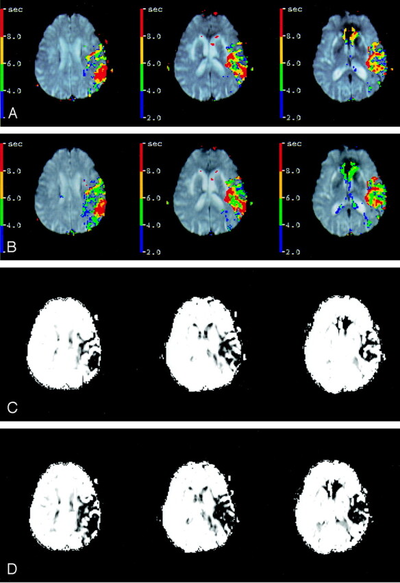
Tmax and CBF maps, created on the basis of the manual (A, C) and automated (B, D) AIFs from Figure 1, have spatial pattern correlations of r = 0.87 and r = 0.86, respectively. Distance between corresponding AIF voxels, or d, is 30.6 mm.

Fig 4.

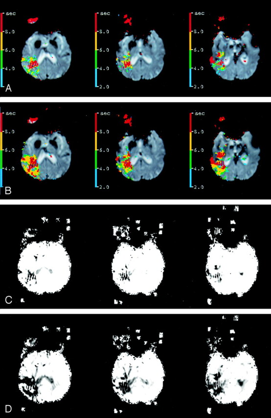
Tmax and CBF maps (A, C) and (B, D) corresponding to Figure 2 have spatial pattern correlations of r = 0.74 and r = 0.60, respectively.

Results

General Characteristics

We examined 22 consecutive patients with acute stroke (12 men, 10 women; mean age ± standard deviation [SD], 72 ± 14 years, age range, 33–90 years) who underwent both DWI and PWI within 24 hours (13 ± 5 hours; range, 5–24 hours) of symptom onset. Two patients had no new lesions on DWI or conventional MR imaging, nine patients had one new lesion, and 11 patients had more than one new lesion.

The manual AIF (identified by D.C.T.) and the auto-AIF on the hemisphere contralateral to the lesion or the expected one were chosen for each patient on the basis of the PWIs (Figs 1A and 2A). For each AIF, 12 Tmax and 12 CBF maps (one of each per section) were created. All maps were considered technically adequate.

Anatomic Locations of AIF Voxels

A single blinded investigator (D.C.T.) evaluated the anatomic locations of the optimized AIF. In all cases, they were considered appropriate (high amplitude, small width, fast decay, and Gaussian-like shape) and always within the MCA territory, although they generally did not correspond to the location of the MCA itself (Figs 1B and 2B). No major venous sinuses were included in any of these regions of interest.

Time to Calculate PWI Maps

The total mean time to identify the AIF manually included the time to identify four appropriate AIFs and picking the best one from the group. This time was significantly longer (85 ± 40 seconds; range, 45–175 seconds) than that needed to run the program on a 1.2-GHz personal computer (13 ± 2 seconds; range, 10–16 seconds).

Quantitative Results

Auto-AIF peaks were significantly higher than the manually derived ones. The mean difference between the two A₀ measurements was 16.16 ± 13.49 seconds⁻¹ (P < .001; 95% confidence interval: 10.18, 22.13 seconds⁻¹), with mean values of 51.89 ± 10.66 and 35.74 ± 9.31 seconds⁻¹. The time to peak identified with an auto-AIF was also earlier than with a manual measurement; however, this difference was not significant (median, 32.22 and 32.50 seconds, respectively; Wilcoxon test statistic W = 46, P = .374). In addition, the width of auto-AIFs was narrower than of the manual ones (median, 2.96 and 3.125 seconds, respectively; W = 116, P = .018) (Table).

Comparison of automated and manual AIF parameters

Subject	ΔA0 (sec−1)	ΔA1 (sec)	ΔA2 (sec)	d (mm)	Correlation r*
					Tmax	CBF
1	21.52	0.69	0.34	11.3	0.91	0.94
2	17.09	1.32	−0.17	15.9	0.87	0.92
3	0	0	0	0.9	1.00	1.00
4	19.75	−0.59	−0.37	7.1	0.82	0.66
5	47.48	−2.98	−1.23	11.4	0.70	0.60
6	11.39	0.32	−0.88	32.2	0.82	0.72
7	29.06	−0.39	−1.28	18.9	0.68	0.74
8	37.22	0.57	−0.68	18.2	0.76	0.83
9	12.83	0.12	0.76	6.0	0.75	0.72
10	32.61	1.30	−0.39	18.2	0.81	0.87
11	25.22	−0.79	−0.17	30.6	0.87	0.86
12	−4.32	−2.65	−2.15	35.9	0.81	0.82
13	1.24	−0.24	−0.30	37.8	0.73	0.82
14	27.30	−2.46	−0.24	24.0	0.74	0.60
15	15.26	−0.19	−0.07	3.0	0.85	0.88
16	17.83	0.36	1.36	2.7	0.80	0.77
17	2.71	−5.25	−2.18	35.0	0.54	0.68
18	0	0	0	1.3	1.00	1.00
19	19.27	−0.62	−0.09	16.9	0.87	0.87
20	11.78	0.71	−0.87	44.5	0.82	0.89
21	10.17	−0.19	−0.30	11.6	0.85	0.87
22	0	0	0	1.3	1.00	1.00
Mean	16.16	−0.50	−0.41	17.5	0.82	0.82
SD	13.49	NA	NA	13.45	0.11	0.12
P value	<0.001	0.374	0.018	NA	NA	NA

Note.—Differences were computed as the automated AIF parameter − manual AIF parameter. A₀ = curve height (maximum concentration of contrast agent), A₁ = curve center (time to peak), A₂ = curve width, d = distance between automated and manual AIF pixels, NA = not applicable.

^*Between automated and manual maps.

We also compared, on a pixel-by-pixel basis, the spatial patterns of manual versus automatically derived Tmax and CBF maps. We performed 528 cross-correlations of different paired maps. Pixel-by-pixel Pearson correlation of maps showed high overall correspondence in their spatial patterns: for Tmax, r = 0.82 ± 0.11 (range, 0.31–1.00), and for CBF, r = 0.82 ± 0.12 (range, 0.13–1.00). Reliability for the automatic method in reproducing the AIFs and maps between repetitive measurements was high (r = 1.0).

The distance between manually and automatically derived AIF voxels was 17.5 ± 13.5 mm, (range, 0.9–44.5 mm). The association between the strength of correspondence in the manually and automatically derived maps and the distance between corresponding AIF voxels was weak for Tmax maps (correlation coefficient r = −0.495, coefficient of determination R² = 0.245, P = .0191,) and it was not significant for CBF maps (r = −0.263, R² = 0.0691, P = .237).

Discussion

We developed an automated computerized algorithm to identify AIF for use in PWI and demonstrated that the algorithm can reliably and accurately identify AIF voxels for perfusion-weighted MR maps. Automation of this process could dramatically reduce PWI analysis time and increase the consistency of PWI analysis, allowing for more practical use of PWI to evaluate patients with ischemic stroke in clinical settings.

We compared our computerized algorithm with conventional manual identification methods to generate AIF curves. Gaussian parameters, along with Tmax and CBF maps, were computed and quantitatively compared. In all cases, the computer-derived AIF curve possessed superior characteristics, including greater amplitude and smaller width, which suggests fewer partial-volume averaging and bolus dispersion artifacts than on the manually identified AIF curve. In addition, the computer-identified AIF appeared to be localized in the territory of the MCA, consistent with established vascular anatomy. The program selects the voxel on the basis of the early timing and high amplitude of the intensity change. This should improve the ability of the program to reject artifacts from venous structures. Consistent with this, no venous structures were included in the AIF voxel in the 22 test cases. In addition, we found no significant association between the strength in correspondence in paired Tmax and CBF maps obtained with both techniques and the distance between the corresponding AIF voxels. This finding suggests that the approach of choosing the AIF on the basis of the dynamics of the flow of contrast agent into the voxel did not introduce a systematic error due to its anatomic proximity to the referenced (manual) AIF voxel. The AIF program also effectively discriminated between changes in signal intensity related to the passage of a contrast-agent bolus from unrelated artifactual noise. Moreover, reproducibility of measurements was high, which indicates that the algorithm is robust and reliable. These characteristics are extremely desirable for producing robust PWI maps.

Carroll et al (23) reported an alternative approach to this problem. Their method concentrated on temporal intensity changes rather an anatomic location. With their technique of automated AIF generation, a single voxel is chosen to represent the AIF on the basis of the arrival time of contrast medium and integrated signal-intensity change in the voxel. In contrast, our method used timing of the intensity peak as a discriminatory criterion, which we assumed should represent both the arrival time (proximal flow dynamic) and the local flow dynamic from this time point to the peak. In addition, our approach does not require analysis of the precontrast points. Carroll et al used integration of the changes in signal intensity over several seconds to minimize confounding effect of transient signal intensity changes due to noise. Our approach, by using a floor threshold for curve width in addition to a goodness-of-fit test, worked as effectively.

Several other groups (24–26) reported different approaches to the analysis of the AIF curves: estimating of arterial likelihood metrics, deriving the mean and SD of the fitted curve parameters, and defining local input functions. A comprehensive intermethod validation study would be valuable to compare the performance of the different algorithms in terms of sensitivity, specificity, validity, and reliability, as well as the feasibility of their use in the clinical settings.

The use of an automated AIF algorithm may have substantial value in the evaluation of patients with acute stroke. It can be used to eliminate off-line postprocessing of dynamic susceptibility contrast MR images, eliminating the need for specially trained personnel and eliminating selection bias. Automation of the AIF acquisition is an important step toward achieving a completely automatic process for generating PWI maps. Such a method could greatly improve the practical use of PWI, particularly in the acute stroke setting when time is critical.

Visual comparison and cross-correlations of the manual and automatic Tmax and CBF maps showed a high degree of spatial pattern correspondence (r = 0.82 ± 0.11 and r = 0.82 ± 0.12, respectively). However, further prospective studies are needed to verify the performance of the algorithm, its usability, and its robustness in the variety of cases (e.g., severe stenosis, strokes in different vascular territories), as well as to analyze and explain the increased discrepancies in the corresponding maps in terms of sensitivity and specificity and relative to other clinical findings. In the future studies, we should not limit regions of interest to the particular circulation. In addition, performance for other types of blood flow maps should be tested. Repetitive manual measurements should be done, and more than one observer should participate to estimate and compare intrarater and interrater reliability.

Our study is subject to a number of limitations. First, because the technique was tested in limited number of patients, it requires verification in a larger sample, ideally one with extremes of PWI changes. In addition, its reliability in the posterior circulation must be verified. Last, as with all MR imaging–based studies, the PWI measured is relative and therefore subject to inaccuracy in individuals with proximal occlusive disease. However, all of these biases are present in manually derived MR imaging–based PWI measurements and intrinsic problems with MR imaging–based techniques.

Conclusion

The results of this validation study suggest that our algorithm for automatically identifying the AIF can create reliable and accurate Tmax and CBF maps. Automation of this process dramatically reduces analysis time and increases the consistency of PWI analysis. In clinical settings, the treating physician can spend less time interacting with the software package (selecting the correct section where the MCA is located) and hence has more time to interact with the patient or to make early treatment decisions.

References

- 1.Runge VM, Clanton JA, Herzer WA, et al. Intravascular contrast agents suitable for magnetic resonance imaging. Radiology 1984;153:171–176 [DOI] [PubMed] [Google Scholar]
- 2.Strich G, Hagan PL, Gerber KH, Slutsky RA. Tissue distribution and magnetic resonance spin lattice relaxation effects of gadolinium-DTPA. Radiology 1985;154:723–726 [DOI] [PubMed] [Google Scholar]
- 3.Villringer A, Rosen BR, Belliveau JW, et al. Dynamic imaging with lanthanide chelates in normal brain: contrast due to magnetic susceptibility effects. Magn Reson Med 1988;6:164–174 [DOI] [PubMed] [Google Scholar]
- 4.Kaneoke Y, Furuse M, Yoshida K, Saso K, Ichihara K, Motegi Y. Transfer index of MR relaxation enhancer: a quantitative evaluation of MR contrast enhancement. AJNR Am J Neuroradiol 1989;10:329–333 [PMC free article] [PubMed] [Google Scholar]
- 5.Kent TA, Quast MJ, Kaplan BJ, et al. Cerebral blood volume in a rat model of ischemia by MR imaging at 4.7 T. AJNR Am J Neuroradiol 1989;10:335–338 [PMC free article] [PubMed] [Google Scholar]
- 6.Moseley ME, Mintorovitch J, Cohen Y, et al. Early detection of ischemic injury: comparison of spectroscopy, diffusion-, T2-, and magnetic susceptibility-weighted MRI in cats. Acta Neurochir Suppl (Wien) 1990;51:207–209 [DOI] [PubMed] [Google Scholar]
- 7.Rosen BR, Belliveau JW, Vevea JM, Brady TJ. Perfusion imaging with NMR contrast agents. Magn Reson Med 1990;14:249–265 [DOI] [PubMed] [Google Scholar]
- 8.Kucharczyk J, Mintorovitch J, Asgari HS, Moseley M. Diffusion/perfusion MR imaging of acute cerebral ischemia. Magn Reson Med 1991;19:311–315 [DOI] [PubMed] [Google Scholar]
- 9.Moseley ME, Kucharczyk J, Mintorovitch J, et al. Diffusion-weighted MR imaging of acute stroke: correlation with T2-weighted and magnetic susceptibility-enhanced MR imaging in cats. AJNR Am J Neuroradiol 1990;11:423–429 [PMC free article] [PubMed] [Google Scholar]
- 10.Edelman RR, Mattle HP, Atkinson DJ, et al. Cerebral blood flow: assessment with dynamic contrast-enhanced T2*-weighted MR imaging at 1.5 T. Radiology 1990;176:211–220 [DOI] [PubMed] [Google Scholar]
- 11.Warach S, Li W, Ronthal M, Edelman RR. Acute cerebral ischemia: evaluation with dynamic contrast-enhanced MR imaging and MR angiography. Radiology 1992;182:41–47 [DOI] [PubMed] [Google Scholar]
- 12.Sorensen AG, Buonanno FS, Gonzalez RG, et al. Hyperacute stroke: evaluation with combined multisection diffusion-weighted and hemodynamically weighted echo-planar MR imaging. Radiology 1996;199:391–401 [DOI] [PubMed] [Google Scholar]
- 13.Calamante F, Thomas DL, Pell GS, Wiersma J, Turner R. Measuring cerebral blood flow using magnetic resonance imaging techniques. J Cereb Blood Flow Metab 1999;19:701–735 [DOI] [PubMed] [Google Scholar]
- 14.Ostergaard L, Weisskoff RM, Chesler DA, et al. High resolution measurement of cerebral blood flow using intravascular tracer bolus passages, part I: mathematical approach and statistical analysis. Magn Reson Med 1996;36:715–725 [DOI] [PubMed] [Google Scholar]
- 15.Ostergaard L, Sorensen AG, Kwong KK, et al. High resolution measurement of cerebral blood flow using intravascular tracer bolus passages, part II: experimental comparison and preliminary results. Magn Reson Med 1996;36:726–736 [DOI] [PubMed] [Google Scholar]
- 16.Wirestam R, Andersson L, Ostergaard L, et al. Assessment of regional cerebral blood flow by dynamic susceptibility contrast MRI using different deconvolution techniques. Magn Reson Med 2000;43:691–700 [DOI] [PubMed] [Google Scholar]
- 17.Calamante F, Gadian DG, Connelly A. Quantification of perfusion using bolus tracking magnetic resonance imaging in stroke: assumptions, limitations, and potential implications for clinical use. Stroke 2002;33:1146–1151 [DOI] [PubMed] [Google Scholar]
- 18.Lythgoe DJ, Ostergaard L, Williams SCR, et al. Quantitative perfusion imaging in carotid artery stenosis using dynamic susceptibility contrast-enhanced magnetic resonance imaging. Magn Reson Imaging 2000;18:1–11 [DOI] [PubMed] [Google Scholar]
- 19.Thijs VN, Somford DM, Bammer R, et al. Influence of arterial input function on hypoperfusion volumes measured with perfusion-weighted imaging. Stroke 2004;35:94–98 [DOI] [PubMed] [Google Scholar]
- 20.Latchaw RE, Yonas H, Hunter GJ, et al. Guidelines and recommendations for perfusion imaging in cerebral ischemia: a scientific statement for healthcare professionals by the writing group on perfusion imaging, from the Council on Cardiovascular Radiology of the American Heart Association. Stroke 2003;34:1084–1104 [DOI] [PubMed] [Google Scholar]
- 21.Rausch M, Scheffler K, Rudin M, Radu EW. Analysis of input functions from different arterial branches with gamma variate functions and cluster analysis for quantitative blood volume measurements. Magn Reson Imaging 2000;18:1235–1243 [DOI] [PubMed] [Google Scholar]
- 22.Calamante F, Gadian DG, Connelly A. Delay and dispersion effects in dynamic susceptibility contrast MRI: simulations using singular value decomposition. Magn Reson Med 2000;44:466–473 [DOI] [PubMed] [Google Scholar]
- 23.Carroll TJ, Rowley HA, Haughton VM. Automatic calculation of the arterial input function for cerebral perfusion imaging with MR imaging. Radiology 2003;227:593–600 [DOI] [PubMed] [Google Scholar]
- 24.Morris ED, VanMeter JW, Tasciyan TA, Zeffiro TA. Automated determination of the arterial input function for quantitative MR perfusion analysis. Presented at: 8th Scientific Meeting of the International Society for Magnetic Resonance in Medicine, Denver, CO, April 3–7,2000
- 25.Reishofer G, Bammer R, Moseley ME, Stollberger R. Automatic arterial input function detection from dynamic contrast enhanced MRI data. Presented at: 11th Scientific Meeting of the International Society for Magnetic Resonance in Medicine, Toronto, Ontario, Canada, July 10–16,2003
- 26.Alsop DC, Wedmid A, Schlaug G. Defining a local input function for perfusion quantification with bolus contrast MRI. Presented at: 10th Scientific Meeting of the International Society for Magnetic Resonance in Medicine, Honolulu, HI, May 18–24,2002