Regional, Layer, and Cell-Type-Specific Connectivity of the Mouse Default Mode Network

Summary

The evolutionarily conserved default mode network (DMN) is a distributed set of brain regions coactivated during resting states that is vulnerable to brain disorders. How disease affects the DMN is unknown, but detailed anatomical descriptions could provide clues. Mice offer an opportunity to investigate structural connectivity of the DMN across spatial scales with cell-type resolution. We co-registered maps from functional magnetic resonance imaging and axonal tracing experiments into the 3D Allen mouse brain reference atlas. We find that the mouse DMN consists of preferentially interconnected cortical regions. As a population, DMN layer 2/3 (L2/3) neurons project almost exclusively to other DMN regions, whereas L5 neurons project in and out of the DMN. In the retrosplenial cortex, a core DMN region, we identify two L5 projection types differentiated by in- or out-DMN targets, laminar position, and gene expression. These results provide a multi-scale description of the anatomical correlates of the mouse DMN.

Graphical Abstract

Highlights

• •Mouse resting-state default mode network anatomy described at high resolution in 3D
• •Systematic axon tracing shows cortical DMN regions are preferentially interconnected
• •Layer 2/3 DMN neurons project mostly in the DMN; layer 5 neurons project in and out
• •Retrosplenial cortex contains distinct types of in- and out-DMN projection neurons

The default mode network is vulnerable to brain disorders, but details of its anatomy and connectivity are coarse. Whitesell et al. use modern neuroanatomical tools in the mouse, including whole-brain imaging and viral tracing, to provide high-resolution anatomical descriptions and identify cell type correlates of this conserved brain network.

Introduction

Large-scale brain networks support sensory perception, cognition, and motor output. Some networks, called resting state (rs) networks, have less well-defined functions and are characterized by temporally correlated intrinsic activity. The rs default mode network (DMN) emerges through rs functional magnetic resonance imaging (rsfMRI) as an anatomically distributed set of brain regions with low-frequency correlated activity in the absence of a goal-directed task (Raichle, 2015). DMN analogs have been identified in monkeys (Vincent et al., 2007), rats (Lu et al., 2012; Upadhyay et al., 2011), and mice (Gozzi and Schwarz, 2016; Grandjean et al., 2020; Sforazzini et al., 2014; Stafford et al., 2014). Conservation of this network across mammalian species suggests a central role in organizing healthy brain activity. Indeed, the DMN is particularly vulnerable in Alzheimer’s disease (AD), showing early accumulation of amyloid deposits and network dysfunction (Buckner et al., 2008; Greicius et al., 2004; Jones et al., 2016; Seeley et al., 2009). The DMN encompasses high-centrality hub regions (Buckner et al., 2008; Liska et al., 2015) that may serve as vulnerability points for psychiatric disorders such as autism and schizophrenia (van den Heuvel and Sporns, 2013; Menon, 2011).

The brain regions that comprise the human DMN are predominantly cortical, symmetric across hemispheres, and broadly distributed in anterior and posterior regions, including the medial prefrontal, precuneus, posterior cingulate, retrosplenial (RSP), and lateral posterior parietal cortex (Buckner et al., 2008; Raichle et al., 2001). Areas outside of the neocortex are also sometimes considered part of the DMN; e.g., the entorhinal cortex, hippocampus, and thalamic nuclei (Alves et al., 2019; Fransson, 2005; Ward et al., 2014). In the human brain, diffusion tensor imaging of fiber tracts has revealed direct structural connections between DMN regions, significantly correlated with functional connectivity (Greicius et al., 2009; Hagmann et al., 2008; Horn et al., 2014). Still, our understanding of the anatomical basis of the DMN is severely limited by the relative coarseness of connectome mapping in humans.

Higher-resolution connectomes based on tracer injections are available for other species in which DMN analogs exist (Bota et al., 2015; Harris et al., 2019; Markov et al., 2014a; Oh et al., 2014; Zingg et al., 2014). These datasets provide quantitative and directional measures of connections at the mesoscale, a level spanning regions, cell populations, classes, and types (Bohland et al., 2009). Analyses at this level reveal conserved rules of cortical connectivity across species (Goulas et al., 2019), including cell-class-specific projection patterns (Harris and Shepherd, 2015), hierarchical organization (Felleman and Van Essen, 1991; Harris et al., 2019), and modular network architecture with some very highly connected nodes (“hubs”; Coletta et al., 2020; van den Heuvel et al., 2016; Rubinov et al., 2015; Swanson et al., 2018; Zingg et al., 2014). Structural connectivity is also generally well correlated with functional connectivity in non-human species (Grandjean et al., 2017; Hutchison and Everling, 2012; Sethi et al., 2017), and comparisons within the DMN have revealed direct anatomical connections between areas (Andrews-Hanna et al., 2010; Coletta et al., 2020; Grandjean et al., 2017; Mantini et al., 2011; Stafford et al., 2014). However, the correspondence is not 1:1. Because brain regions participate in multiple, partially overlapping functional networks, multiplexing may instead be achieved at the level of cell populations or types.

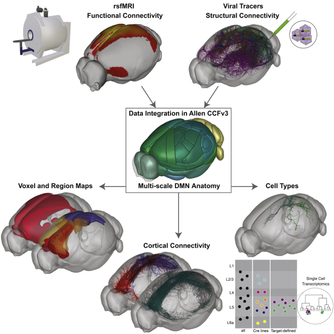
Cross-species conservation of structural connectivity rules and rs networks suggests that we can gain relevant insights into the anatomy of human functional networks by studying animal models (Díaz-Parra et al., 2017; Stafford et al., 2014). Here we provide a detailed spatial description of the brain regions and connections in the mouse DMN. We registered a rsfMRI DMN mask with the fully annotated 3D Allen Mouse Common Coordinate Framework Reference Atlas version 3 (CCFv3; Wang et al., 2020), allowing integrated analyses of the DMN with regional and cell-type-specific anterograde axonal tracing experiments from the Allen Mouse Brain Connectivity Atlas (MCA; Harris et al., 2019; Oh et al., 2014). We found that voxels and regions within the DMN are preferentially connected to other DMN regions. Using Cre-defined tracing data, we show how axonal projections from layer 2/3 (L2/3) DMN neurons target other DMN regions, whereas L5 neurons target areas in and out of the DMN. Individual L5 neurons could send axonal branches to targets in and out of the DMN, broadcasting information to multiple downstream targets. Alternatively, specific types of projection neurons may preferentially target in- or out-DMN regions. To test these possibilities, we used a dual retrograde/anterograde intersectional viral tracing method (Gore et al., 2013) to label all axon branches from neurons defined by one target. We found strong evidence for in- and out-DMN projection types in the ventral RSP and further characterized them using single-cell transcriptomics.

Results

Spatial Maps of the Mouse DMN at Voxel and Regional Levels

To identify the DMN, we performed blood-oxygen-level-dependent (BOLD) rsfMRI experiments on lightly anesthetized mice (Gutierrez-Barragan et al., 2019). We found five rs networks (“components”) using low-dimensional group independent component analysis (ICA). Four matched previously described networks (Sforazzini et al., 2014): (1) default mode, (2) somatomotor, (3) lateral cortical, and (4) hippocampal. The fifth component contained cerebellar signal and noise. We aligned ICA components 1–4 to the Allen CCFv3 (Figure 1A) after thresholding each component at a Z score of 1. The DMN component was also threshholded at a Z score of 1.7 to identify “core” DMN structures. Finally, we symmetrized each component to generate 3D masks registered to the Allen CCFv3 at 100-μm voxel resolution (Figures 1B, 1C, and S1A–S1C).

Figure 1.

Identification of DMN Structures

(A) Workflow for registering fMRI data to the Allen CCFv3. (1) Align the in-house fMRI template to CCFv3. (2) Apply the obtained transform to the ICA components. (3) Threshold at Z = 1 for all masks and Z = 1.7 for the DMN core mask. (4) Symmetrize along the midline. (5) Overlay CCFv3 region boundaries.

(B) 3D image of the ICA DMN component registered to the CCFv3 template.

(C) Serial cutaway images showing the DMN on coronal sections.

(D) 3D views showing the major brain divisions in CCFv3 and pie charts showing the composition by major brain division for DMN and core DMN masks.

(E) Percentage of voxels overlapping the DMN masks within all isocortex structures and selected structures in other major brain divisions. Colored boxes around isocortex structures indicate module affiliation from Harris et al. (2019).

(F) 3D views show spatial locations of DMN regions colored by module (in E).

Abbreviations in Table S1; see also Figure S1 and Tables S2 and S3.

To define the anatomical structures of the DMN, we calculated the percentage of voxels within the CCFv3-aligned DMN mask that overlap with structures annotated in CCFv3. Starting at the major brain division level, we found that most (77.6%) of the voxels in the DMN belong to the isocortex. The rest of the mask voxels (22.3%) are in fiber tracts, the striatum, olfactory areas, and the mediodorsal thalamus (Figure 1D). The core DMN mask is even more restricted to the cortex (89.6%). Overlaps of the other three rs networks with major brain divisions are shown in Figures S1E–S1G. We performed the same calculations for a set of 316 regions brain-wide (i.e., the “summary structure set”; Table S2). We identified 36 isocortical areas with at least one voxel in the DMN mask and 25 areas in the core-DMN mask (Figure 1E). In the thalamus, containing 2% of the total DMN mask, specific structures included several midline nuclei. We chose to conservatively define regions inside the DMN (“in-DMN”) as those with more than 50% of their voxels in the core-DMN mask; only 15 regions in the isocortex passed this threshold (Figure 1E, black bars over thick dashed line). Of note, 4 cortical regions had more than 50% of their voxels inside the Z = 1 but not the Z = 1.7 DMN mask and were considered “out-DMN” regions: the posteromedial and rostrolateral visual areas (VISpm and VISrl) and dorsal and ventral agranular insular cortex (AId and AIv). The core mask was used only to define DMN structures; subsequent analyses used the Z = 1 DMN mask.

We noted a strong resemblance between the spatial patterns of the DMN masks and two of six structural connectivity-based cortical modules we identified previously using a community detection algorithm (Harris et al., 2019). Structures in each module are more strongly connected with each other than with structures in other modules. Most in-DMN structures (n = 12 of 15) belong to prefrontal or medial modules (Figure 1E), and most regions belonging to these two modules were also defined as in-DMN structures. The DMN also included two regions of the somatosensory cortex (trunk and lower limb) and secondary motor cortex (MOs). Locations for all in-DMN regions in CCFv3 space are shown in Figure 1F. In summary, the DMN was anatomically defined most specifically by the voxel-resolution mask, alternatively by a set of 15 cortical regions, and approximately by the combination of the prefrontal and medial modules.

Preferential Region-to-Region Connectivity in the DMN

The assignment of most in-DMN regions to only two modules suggests that connections inside the DMN are stronger than connections made to cortical areas outside of the DMN. To quantify in-DMN preferential connectivity, we used 300 anterograde viral tracer experiments distributed across the cortex in wild-type (WT) mice from the MCA (Oh et al., 2014; Figure 2A). We also included injections in the cortical pan-excitatory Emx1-IRES-Cre line (Emx1) and the Rbp4-Cre_KL100 line (Rbp4) that labels L5 projection neurons because they project to the same cortical targets with connection strengths that are significantly correlated for matched source areas (Harris et al., 2019).

First we measured the strength of axonal projections inside and outside of the DMN mask at voxel-level resolution. For each experiment, we compared the fraction of the injection site in the DMN mask (injection DMN fraction) with the fraction of cortical projections in the DMN mask (projection DMN fraction). We observed a significant positive correlation between these measures (Pearson correlation [r] = 0.94, p < 0.001; Figure 2B). Axonal projections labeled from two injections (100% in or 100% out of the DMN) are shown in Figures 2C–2H.

Figure 2.

DMN Regions Preferentially Project to Other DMN Regions

(A) Top-down view of the cortical surface showing the spatial distribution of the 300 tracing experiments used to quantify fraction of DMN projections (shown by colormap). Gray, DMN mask; black, region boundaries.

(B) Projection DMN fraction as a function of the injection DMN fraction for the experiments in (A). r, Pearson correlation.

(C and D) Cortical projection images showing axons arising from an experiment inside (C, ACAd) and outside of (D, VISp) the DMN mask. Asterisks indicate the approximate injection centroid. Cyan, in-DMN projections; green, out-DMN projections. Experiment IDs: ACAd, http://connectivity.brain-map.org/projection/experiment/cortical_map/112458114; VISp, http://connectivity.brain-map.org/projection/experiment/cortical_map/100141219. Dashed lines show the location of coronal sections in (E)–(H).

(E–H) Virtual sections of the CCFv3 template overlaid with aligned experiment data at (E and F) the center of each injection site (green pixels with asterisks; E, ACAd; F, VISp) and (G and H) target areas with high axon projection densities (green pixels). Arrows, in-DMN projections; arrowheads, cortical projections outside of the DMN; green edges, isocortex boundary; white overlay, DMN mask; portions overlapping the striatum (STR) and thalamus (TH) are also labeled.

(I) Fraction of cortical projections inside the DMN for experiments in (A), grouped by injection source. Individual points are colored by the percentage of their injection inside the DMN mask.

(J) Points from (I) grouped by in-DMN or out-DMN regions.

(K) Right hemisphere cortical surface flat map showing regions colored by module with DMN mask overlaid (white).

(L) Points from (I) grouped by module affiliation. Boxplots show median and interquartile range (IQR). Whiskers extend to 1.5 × IQR. See also Figure S2.

It is not surprising to find that injections inside the DMN send a higher fraction of their projections to the DMN, given that the mask is spatially continuous (Figures 1B and 1C) and connection density decreases as a function of distance (Markov et al., 2014b; Oh et al., 2014; Ercsey-Ravasz et al., 2013). To estimate how much preferential intra-DMN connectivity can be explained by spatial proximity, we applied a general linear model (GLM) to derive a distance coefficient and a DMN coefficient for each experiment (Figures S2A and S2B). Distance coefficients were negative or close to zero and had a low inverse correlation with the injection DMN fraction (r = −0.16, p = 0.005; Figure S2C). DMN coefficients, however, were positively correlated with the injection DMN fraction (r = 0.60, p < 0.001; Figure S2D). Thus, DMN regions do send more projections to other DMN regions, even after accounting for distance.

To test whether the tendency for regions inside the DMN to send more projections inside that network is unique to the DMN or a more general property of rs networks, we also calculated mask and distance coefficients for the other rs networks. In all cases, injections inside each mask had more cortical projections inside that mask, and injections outside had more cortical projections outside the mask, even after accounting for distance (Figures S2E and S2F). This relationship held for hippocampal injections in the hippocampal network (Figure S2F). In fact, the correlation between injection and projection fractions was stronger for the other cortical networks than for the DMN, suggesting that it may be less preferentially connected, consistent with its polymodal nature (Buckner and DiNicola, 2019).

Next we tested whether preferential connectivity is also observed at the regional level by grouping the 300 isocortex injections into in- or out-DMN brain regions (Figure 1E). Like at the voxel-level, injections into in-DMN regions generally had a higher fraction of DMN projections than injections into out-DMN regions (Figures 2I and 2J). We again used a GLM to separate the effects of distance and DMN connectivity, finding that experiments in most in-DMN structures indeed had positive DMN coefficients, although a few were zero or negative (Figures S2G–S2I).

The DMN mask boundaries do not always align with anatomical boundaries (Figure 2K). Thus, across regions, the injection DMN fraction was more predictive of the projection DMN fraction than whether the source region containing the injection was itself an in-DMN structure (see colormaps for individual points in Figures 2I and 2J). For example, injections in the DMN portion of the MOs had more DMN projections than MOs injections located outside of the DMN (see the bimodal distribution in Figure 2I and Figures S2K–S2R). At a module level, most injections in prefrontal and medial modules had more than 50% of their cortical projections inside the DMN mask (Figure 2L). Conversely, injections in lateral and auditory modules had less than 50% of their cortical projections in the DMN. These results were consistent when accounting for distance (Figure S2J).

A final summary of the cortical regions and projections that intersect the core-DMN mask is provided in Table S2. These results confirm preferential direct connectivity between DMN regions and also suggest that the DMN covers functionally segregable subdivisions of anatomically defined structures.

Preferential Connectivity between DMN Regions by Layer and Projection Cell Class

Although DMN regions are more strongly connected to other DMN regions, they still project outside of the DMN. We hypothesized that anatomical cell types with distinct target specificities might selectively route information within or between networks. Excitatory neurons in the cortex are classified by projection targets and layers into three major classes: intratelencephalic (IT) in L2–L6, pyramidal tract (PT) in L5, and corticothalamic (CT) in L6 (Harris and Shepherd, 2015). Although many corticocortical projections originate from L2/3 and L5, the L5 IT class generally projects to a larger set of targets (Harris et al., 2019). Critically, cells in other layers project to a subset of the L5 cortical targets (Harris et al., 2019). Thus, one possibility is that connections to in- and out-DMN areas are made by L5 cells, whereas IT cells in other cortical layers project specifically to in-DMN targets.

To investigate how layer- and class-specific projection patterns relate to the DMN, we used a published set of spatially matched viral tracing experiments in 14 Cre lines selective for L2/3, L4, L5 IT, L5 PT, and L6 CT classes, plus a WT or Emx1 injection (Harris et al., 2019). Groups were formed around one experiment in the L5 Rbp4 line; the other experiments in a group were located within 500 μm of this Rbp4 “anchor.” We further curated the published anchor groups to ensure that all experiments in the same group were inside or outside of the DMN (STAR Methods; n = 350 experiments in 42 spatially matched groups). We focused primarily on experiments in Cre lines selective for L2/3 (Cux2-IRES-Cre and Sepw1-Cre_NP39) and L5 IT (Rbp4 and Tlx3-Cre_PL56 (Tlx3; Figure 3), but results from L4 IT, L5 PT, and L6 CT experiments are provided (Figure S3). Of note, Cre-dependent viral tracer injections in Rbp4 label L5 IT and L5 PT cells (Harris et al., 2019). We classify the Rbp4 data here as L5 IT because we focused exclusively on intracortical projections, and the PT class has relatively few (Harris and Shepherd, 2015). Cortical projections arising from Cre-defined neuron classes in the anteromedial visual cortex (VISam; a DMN region) highlight some layer-specific cortical projection patterns (Figure 3B). Notably, L2/3 projections visually overlap with L5 output but target fewer regions, particularly in the contralateral hemisphere (Harris et al., 2019; Figure 3B).

Figure 3.

L2/3 Neurons Have More Intra-DMN and Intra-module Projections Than L5 Neurons

(A) Top-down cortical surface view showing the locations of matched anterograde viral tracing experiments in WT and Emx1-IRES-Cre mice (black, n = 41), L2/3 IT Cre driver lines (cyan, n = 46), and L5 IT Cre driver lines (gray, n = 76). Red circle indicates the VISam group. Gray, DMN mask; black, region boundaries.

(B) Cortical projection images from spatially matched experiments in WT (black box), Cux2-Cre (L2/3 IT, cyan box), and Rbp4-Cre and Tlx3-Cre (L5 IT, gray box) mice. Asterisks indicate the approximate injection centroid. Cyan, in-DMN projections; green, out-DMN projections; gray, DMN mask; colored lines, module boundaries. Experiment IDs: WT, http://connectivity.brain-map.org/projection/experiment/cortical_map/100141599; Cux2, http://connectivity.brain-map.org/projection/experiment/cortical_map/184167484; Rbp4, http://connectivity.brain-map.org/projection/experiment/cortical_map/159753308; Tlx3, http://connectivity.brain-map.org/projection/experiment/cortical_map/297233422.

(C) Projection DMN fraction as a function of injection DMN fraction for the 163 experiments in (A). The inset shows the points split into in-DMN and out-DMN bins.

(D–F) Fraction of cortical projections inside the DMN for the L2/3 and L5 experiments grouped by injection source (D), in-DMN or out-DMN sources (E), and module (F).

(G) Boxplots showing the fraction of intra-module projections for experiments in L2/3 IT- and L5 IT-selective Cre lines. Boxplots show median and IQR. Whiskers extend to 1.5 × IQR.

Statistical significance was determined using a multi-way ANOVA followed by Tukey’s post hoc test for group comparison. See also Figure S3.

L2/3 and L5 IT cell classes had significant correlations between the injection and projection DMN fractions (Figure 3C, r = 0.91, 0.96, p < 0.001). Notably, inside the DMN mask, L2/3 had a significantly higher fraction of projections in the DMN than L5 IT (p = 0.007; Figure 3C, inset). The fraction of DMN projections was also significantly higher for L2/3 compared with L5 IT experiments for in-DMN but not out-DMN sources (p = 0.003; Figures 3D and 3E). In fact, almost all of the projections arising from L2/3 inside the DMN target other DMN regions (median = 0.91 compared with 0.73 for L5 IT projections). Because the DMN mask is symmetrical across hemispheres and there are fewer contralateral projections from L2/3 IT neurons, we speculated that the higher fraction of projections in the DMN from L2/3 might be simply explained by this difference. However, removing the contralateral projections from this analysis did not change the relative differences between groups (compare Figure 3C and Figures S3C–S3E with Figures S3F–S3H).

Injections located in prefrontal and medial modules had significantly more DMN projections from L2/3 compared with L5 IT cells (Figure 3F; p = 0.01 prefrontal, p = 0.04 medial). Because the DMN is mainly composed of these two modules, we thought that this difference may reflect an overall tendency for L2/3 IT cells to have a more specific intra-module projection pattern compared with L5 IT cells. We tested this by measuring the fraction of intra-module projections for other modules with n > 1 source region in our dataset. In all cases, L2/3 had a higher fraction of intra-module projections than L5 IT neurons (Figure 3G). These results show that DMN target regions receive input from L2/3 and L5 IT cells in DMN source regions but that projections outside the DMN mask, from DMN sources, arise predominantly from L5 IT cells.

Preferential Connectivity between DMN Regions by Target-Defined Neuron Type

Cre lines are useful for labeling broad cell classes, but many contain a mix of cell types based on transcriptomic, morphological, and physiological properties (Gouwens et al., 2019; Tasic et al., 2016, 2018). So, although, at a population level, L5 IT cells project to areas in and out of the DMN, subclasses could project to these targets in non-random combinations (Chen et al., 2016; Economo et al., 2016; Han et al., 2018). We hypothesized that L5 projection neuron types may co-exist in DMN regions that preferentially target in- or out-DMN regions. To test this, we used an intersectional viral tracing approach to label all collateral axons of target-defined (TD) projection cell types (Gore et al., 2013).

Our experimental approach is illustrated in Figures 4A and 4B. We injected a retrogradely transported canine adenovirus encoding Cre (CAV2-Cre; Hnasko et al., 2006; Soudais et al., 2001) into a “primary target” region and a Cre-dependent adeno-associated virus (AAV-FLEX-EGFP) into a “source” region in Ai75 Cre reporter mice that express nuclear-localized tdTomato (nls-tdT; Daigle et al., 2018). Thus, neurons with axon terminals in the primary target express Cre following retrograde transport and are visible brain-wide as nls-tdT+. In the source, co-infected cells that express Cre (nls-tdT+) will also express EGFP, which fills the cell (including axons), allowing visualization of projections to the primary target and all other targets (“secondary targets”; Figure 4B). TD experiments are named according to their source with a subscript indicating their primary target; i.e., an ACAd_RSPv experiment has an AAV injection into the anterior cingulate area, dorsal part (ACAd) and a CAV2-Cre injection into the ventral RSP cortex (RSPv), so all cells expressing EGFP in that experiment have cell bodies in the ACAd and project to the RSPv. In cases where CAV2-Cre infected two target regions equally, both are listed in the subscript (e.g., ACAd_RSPv/RSPd). Importantly, CAV2-Cre has a tropism bias toward L5 over L2/3 neurons (Chatterjee et al., 2018), but this bias is expected to be in our favor in these experiments (given the L5 IT focus).

Figure 4.

Target-Defined Projection Mapping Differentiates In-DMN and Out-DMN Projections for Sources in the Medial Module

(A and B) Experimental design and terminology.

(A) In a target-defined (TD) experiment, a “source” injection with a Cre-dependent viral tracer (AAV-FLEX-EGFP) is paired with a “primary target” injection of a retrograde virus encoding Cre (CAV2-Cre). In the source, Cre mediates expression of EGFP in co-infected cells, allowing visualization of brain-wide projections, including “secondary targets.” Experiments are done in Ai75 mice so that all cells infected retrogradely with CAV2-Cre express nuclear tdTomato (tdT).

(B) Schematic illustrating three hypothetical TD projection patterns from an in-DMN source paired with an in-DMN (purple) or out-DMN (green) target. Out-DMN TD cells are shown projecting only to other out-DMN regions. In-DMN TD cells may project to a specific (dark purple) or broad (light purple) set of in-DMN targets.

(C) Cortical projection images from Rbp4-Cre+ L5 neurons in ORBl (syringe location).

(D and E) Projections labeled by TD experiments in ORBl paired with an in-DMN target (ACAd, D), or an out-DMN target (VISal, E). Gray, DMN mask; black, region boundaries; cyan, in-DMN projections; green, out-DMN projections. Experiment IDs: ORBl_Rbp4, http://connectivity.brain-map.org/projection/experiment/cortical_map/156741826; ORBl_ACAd, http://connectivity.brain-map.org/projection/experiment/cortical_map/571816813; ORBl_VISal, http://connectivity.brain-map.org/projection/experiment/cortical_map/601804603.

(F) Cortical surface flat map showing the locations of 10 groups of experiments (red circles) with matched injection sites and at least one of each: TD in-target, TD out-target, WT. Gray, DMN mask; black, region boundaries.

(G) Projection DMN fraction as a function of injection DMN fraction for the three experiment types. The inset shows the fraction of DMN projections for injections split into in-DMN and out-DMN bins.

(H–J) Boxplots showing the fraction of projections inside the DMN for the experiments in (F), grouped by source region (H), in-DMN and out-DMN sources (I), and module (J). Boxplots show median and IQR. Whiskers extend to 1.5 × IQR.

Statistical significance was determined using a multi-way ANOVA followed by Tukey’s post hoc test for group comparison. See also Figure S4 and Table S4.

In- and out-DMN primary target locations for a given source were chosen based on analyses of projections labeled in WT, Emx1, or Rbp4 mice. For example, L5 IT axons originating from ORBl project widely to multiple cortical targets (Figures 4C and S4A–S4C), including ACAd (in-DMN) and the anterolateral visual area (VISal; out-DMN). In this example, we paired a source injection in ORBl with CAV2-Cre in ACAd (ORBl_ACAd; Figures 4D and S4D–S4F). ORBl_ACAd cortical projections appeared to be a subset of the total ORBl L5 projection pattern (compare with Figure 4C); axons were densest in the rostral DMN in both hemispheres and also targeted lateral cortical areas outside of the DMN. An ORBl source injection paired with VISal (ORBl_VISal) revealed a different subset of the ORBl L5 projections (Figures 4E and S4G–S4I). These results show that TD projection mapping can reveal intracortical projection neuron types with distinct multi-area targeting patterns.

We sought to identify TD experiments with “specific” (i.e., few secondary targets) as opposed to “broad” projection patterns (Figure 4B) based on the assumption that limited target patterns are more likely to be formed by a distinct subclass of neurons. Note that TD experiments have a smaller volume of infected cells than WT or Cre tracer experiments (Figure S5A) and so may be expected to contact fewer targets, particularly when the larger injections result in infection across borders into secondary sources. Thus, to be certain that each TD experiment could reasonably be expected to represent a subset of the WT projections, we only compared experiments that met four criteria: (1) the source structure was the same; (2) if the source structure was less than 60% of the injection volume in either experiment, then the structure containing the second-highest fraction of the source injection was also the same; (3) injection centroids were ≤ 800 μm apart; and (4) the injection spatial overlap (Dice coefficient) was more than 0.05. Using these criteria, we identified 10 sets of injection-matched cortical experiments comprised of at least one experiment per type: (1) TD, in-DMN target; (2) TD, out-DMN target; and (3) a WT, Emx1, or Rbp4 L5 experiment (STAR Methods). This curated set includes data for 10 cortical areas (Figure 4F) with 105 total experiments (63 TD and 42 WT) in 8 (of 15) in-DMN and 2 out-DMN sources. Experiment IDs are provided in Table S3.

We used this rigorously curated dataset to test our hypothesis that different L5 projection neuron types in DMN regions target sets of in- or out-DMN regions. We again found significant correlations between the injection and projection DMN fractions (r = 0.94 TD in-target, 0.96 out-target, 0.95 matched WT, all p < 0.001; Figure 4G). Overall, there was no difference in the fraction of in-DMN projections for sources paired with in-DMN targets compared with out-DMN targets (Figures 4H and 4I). However, we were intrigued to observe considerable variability in the DMN projection fraction for in-DMN source experiments, particularly when paired with out-DMN targets (white boxplot for in-DMN sources in Figure 4I). Grouping the sources by module highlighted a difference between prefrontal and medial sources (Figure 4J). Sources in the prefrontal module sent a high fraction of their projections to the DMN regardless of whether they were paired with an in-DMN or out-DMN target. In contrast, sources in the medial module had a significantly higher fraction of projections inside the DMN when paired with in-DMN compared with out-DMN targets (p < 0.05). The high fraction of DMN projections from prefrontal sources regardless of their primary target is consistent with a hub-like configuration of this polymodal region, whereas the higher in-DMN fraction for medial sources paired with in-DMN targets implies the presence of separate in-DMN- and out-DMN-projecting cell types in medial regions.

TD Regional Projection Patterns Vary by Source and Module

TD experiments project to significantly fewer targets than their WT matches (n = 33 ± 17 versus 63 ± 21, p < 0.001, Student’s t test; Figure S5B), but even with the match criteria above, the size difference between WT and TD injection volumes remained a confound for quantitative comparisons (Figure S5C, left). We therefore constructed a model to identify TD experiments with projection patterns that differ from the WT. We used a large set of WT replicates to predict the Spearman correlation (r_s) for two experiments based on the volume of the smaller injection in the pair, the distance between the two centroids, and the overlap between the two injection sites (Figure S5D; STAR Methods). We used this model to calculate the predicted r_s for each WT-TD pair and then identified pairs below the 95% prediction interval as less correlated than expected for replicate injections (Figure S5D). We call these “low corr” pairs. Some source structures had a higher fraction of low corr pairs than others (e.g., ORBl, ACAv, and ORBvl; Figures 5A and S5E). Specific examples of WT-TD pairs are shown in Figures S5F–S5H. Many sources in our dataset, like ACAd, had 0 low corr pairs, whereas others, like VISp and RSPv, had an intermediate fraction (more examples in Figure S6). One of the VISp low corr pairs included the target VISl (VISp_VISl), which labeled projections resembling an LI-LM-PM projection type observed using sequence-based connectivity mapping (Han et al., 2018). Notably, r_s values were significantly lower for low corr pairs in the prefrontal and medial compared with the visual module and in the medial compared with the prefrontal module (Figure 5B; p < 0.02, one-way ANOVA followed by multiple t tests).

Figure 5.

Quantitative Comparisons of TD and WT Injection-Matched Pairs

(A) Sources ranked by the fraction of low corr pairs (left; top axis, black circles; bottom axis, number of pairs). Right: mean r_s (top axis) for low corr (white circles) and non-low corr (black circles) WT-TD pairs. The numbers of total pairs (left) and low corr pairs (right) are plotted on bottom axes in gray.

(B) Distribution of r_s values for low corr pairs grouped by module. Boxplots show median and IQR. Whiskers extend to 1.5 × IQR. Statistical significance was determined using a one-way ANOVA followed by multiple t tests.

(C–K) Cortical projection images (C, F, and I) and coronal section serial two-photon tomography (STPT) images through the source (D, G, and J) and target (E, H, and K) injection sites for three experiments in the RSPv. Bars on the bottom of (E), (H), and (K) show the fraction of the CAV2-Cre injection site in each brain region. In-DMN PL and ACAd targets (C–H)) reveal midline-projecting patterns, whereas out-DMN VISl and VISp targets (I–K) reveal a visually projecting pattern.

(L) Overlay of the cortical projection images from (C), (F), and (I).

(M) Cortical projection image from a matched RSPv WT injection. Experiment IDs: RSPv_PL, http://connectivity.brain-map.org/projection/experiment/cortical_map/592522663; RSPv_ACAd, http://connectivity.brain-map.org/projection/experiment/cortical_map/521255975; RSPv_VISl/VISp, http://connectivity.brain-map.org/projection/experiment/cortical_map/569904687; RSPv_WT, http://connectivity.brain-map.org/projection/experiment/cortical_map/112595376. Gray, DMN mask; Black, region boundaries.

(N) Projection strengths (log-transformed normalized projection volume [NPV]) to selected targets, plotted for each TD projection type.

(O) Projection strengths to all targets in the prefrontal, medial, and visual modules. Statistical significance was determined using a multi-way ANOVA followed by Tukey’s post hoc test for group comparison.

Axes in (N) and (O) are truncated at 10^−2.5. See also Figures S5 and S6 and Table S5.

Two DMN-Related TD Projection Patterns in RSPv

The r_s for low corr pairs in RSPv, a core-DMN region, were some of the smallest in the dataset (white points in Figure 5A, right). So we next asked whether these specific TD projection patterns relate to the DMN. We identified a midline-projecting pattern in RSPv_PL and RSPv_ACAd experiments (Figures 5C–5H and S5H). In contrast, projections from RSPv_VISp and RSPv_VISl/VISp experiments had a different portion of the WT pathway labeled; i.e., a visually projecting pattern (Figures 5I–5K). These projection types contact distinct subsets of WT targets (Figures 5L and 5M); midline-projecting experiments primarily reach in-DMN targets and visually projecting experiments reach more out-DMN targets.

Although these two labeled pathways are mostly non-overlapping, some axons were detected in the same target regions. Quantitative comparison showed that midline-projecting experiments, particularly RSPv_PL, had stronger connectivity to prefrontal targets compared with visually projecting RSPv_VIS experiments (Figures 5N and 5O). Conversely, visually projecting RSPv cells had stronger projections to targets in the visual module than midline-projecting types (Figure 5O). Indeed, most visual areas received little to no input from midline-projecting types, with the exception of the posterior-lateral visual area (VISpl), to which nearly all experiments projected (Figure 5N).

Notably, we found the midline DMN-projecting pattern only in the ventral caudal RSPv (analogous to A29a,b in the rat; Sugar et al., 2011; Vogt and Paxinos, 2014; Figures S7A–S7D). Midline-projecting cells were also labeled in a ventral caudal RSPv TD injection paired with the VISpl and medial entorhinal cortex (ENTm) but not with the VISpl alone (Figure S7C versus S7D). Because of the known tropism bias of CAV2-Cre to L5 neurons, we confirmed that midline-projecting (RSPv_ACAd and RSPv_VISpl) and visually projecting (RSPv_VISp) cells were also labeled with another retrograde rabies virus, RVΔGL-Cre, without this bias (Chatterjee et al., 2018; Figures S7E–S7G). Critically, RVΔGL-Cre experiments labeled many more L5 than L2/3 cells (Figure S7H), indicating that L2/3 cells do not contribute in a major way to these two projection-types.

We noted that the midline-projecting RSPv injections appeared to label L5 cells located superficially to those in visual-projecting experiments (Figures 6A and 6B). CCFv3 registration placed most source cells from all experiments in L5, but midline-projecting experiments had some signal assigned to L2/3, and visually projecting experiments had slightly more signal assigned to L6 (Figure 6C). Small variances in registration precision might result in mis-assignment of voxels in deep L2/3 to L5 or vice versa. We therefore confirmed the sublayer locations of these projection types by comparing the distribution of tdT expression in 4 cortical layer-selective Cre driver lines crossed to the Ai14 reporter line (Figures 6D–6H) with the distribution of EGFP fluorescence levels inside the TD injection sites (Figure 6H, right). The peaks of the distributions were located ∼40% (midline-projecting) and 60% (visually projecting) of the relative distance from the pia to the white matter, a range more like the L4/5 and L5 Cre lines (Scnn1a and Rbp4) than the L2/3 (Cux2) or L6 (Ntsr1) line. These plots suggest that both projection types are indeed in L5 but that midline-projecting neurons are located in a sublayer above most of the visually projecting population.

Figure 6.

Midline-Projecting RSPv Cells Are Located in Superficial L5

(A) Overlay of STPT images from the RSPv TD source injection sites in Figures 5C–5K. Dashed lines show manually drawn layers.

(B) A coronal CCFv3 atlas plate shows layer annotations in the caudal portion of the RSPv.

(C) Source layers with infected cells, determined by registration to CCFv3.

(D–G) STPT images of tdT expression from a set of layer-selective Cre lines (indicated in each panel) crossed to the Ai14 reporter. tdT+ somas are in L6 of the Ntsr1-Cre × Ai14 line, but projections are dense in L5 (G).

(H) Plots showing fluorescence levels by depth from the pia to the white matter for the layer-selective Cre × Ai14 lines (tdT, left) and the TD source injection sites (EGFP, right).

(I) Single coronal STPT images of cells in the RSPv labeled following from retrograde trans-synaptic rabies tracing experiments in PL (magenta, left), ACAd (cyan, left), or VISp (green, center). White boxes indicate regions shown in the merged overlay on right (rotated with L1 at the bottom).

See also Table S6.

We further validated the sublaminar locations of these projection types in the RSPv with data generated by monosynaptic cell-type-specific rabies tracing experiments. We injected a Cre-dependent AAV (expressing the EnvA TVA receptor, tdT, and rabies glycoprotein), followed by an EnvA-pseudotyped, glycoprotein-deleted rabies virus expressing nuclear-localized EGFP into the prelimbic area (PL), ACAd, or VISp of Rbp4-Cre mice (Lo et al., 2019). RSPv L5 cells were labeled in all three cases. Cells projecting to the PL were indeed superficial to cells projecting to the VISp. ACAd projecting cells were intermingled or between PL- and VISp-projecting cells in these experiments (Figure 6I). We conclude that there are at least two projection types in RSPv L5: one that primarily projects to DMN targets (midline-projecting) and a second that primarily projects to visual targets (visually projecting).

Correspondence of RSPv Projection Types and Transcriptomic Types

To determine how the different RSPv projection types relate to transcriptomically defined cell types, we performed Retro-seq experiments (retrograde viral tracing combined with single cell sequencing; Tasic et al., 2018; Figure 7A). We injected CAV2-Cre or rAAVretro (Tervo et al., 2016) into the ACA or VISp in Cre reporter mice (Ai14, Ai75). We then isolated cells from the caudal part of the RSPv for single-cell transcriptomic profiling using SMART-Seq v.4 (Tasic et al., 2018). We mapped these cells into a recently developed comprehensive cell type taxonomy for the entire mouse isocortex and hippocampal formation (Yao et al., 2020) using gene expression profiles (Figure 7B; STAR Methods). Most midline-projecting cells mapped to a single cluster, 236_L3 RSP-ACA. Notably, many visually projecting cells also mapped to this cluster. We found other transcriptomic types among the visually projecting cells, including 255_L5 PT RSP-ACA (one ACA-projecting cell also mapped to this cluster). Cluster 236 is an unusual subclass. It strongly expresses two L4 marker genes, Scnn1a and Rspo1, one of two L5 PT cell markers (Bcl6 but not Fam84b), and a pan-IT marker, Slc30a3. Yao et al. (2020) concluded that this subclass has an intermediate cell type identity between IT and PT. It was called L3 because of mixed-layer marker gene expression and because there is no anatomically defined L4 in the RSPv. Our results suggest that the location of these cells is more consistent with superficial L5.

Figure 7.

Midline-Projecting and Visually Projecting RSPv Cell Types Have Different Gene Expression Patterns

(A) Retro-seq experiment and analysis design. ACA and VISp-projecting cells in RSPv were labeled by injections of retrograde Cre virus in Ai14 or Ai75 mice. Single tdT+ cells were sorted from the caudal RSPv for RNA sequencing and mapped to clusters in a cortical hippocampal cell type taxonomy. Supervised analyses identified differentially expressed genes (DEGs).

(B) Cluster assignments for 239 cells. Cluster labels are from Yao et al. (2020).

(C) Left: log-normalized gene expression for all female midline-projecting cells (x axis) versus all female visually projecting cells (y axis). Red points indicate DEGs. Center: heatmaps showing the scaled expression (log counts per million [CPM]) of DEGs (rows) for each single cell (columns). Right: violin plots summarizing the population distribution of expression levels for each DEG by target (ACA or VIS).

(D) Same as (C) but limited to female cells in cluster 236_L3 RSP-ACA.

(E) Coronal section image showing ISH for Arc in the RSPv from the Allen Mouse Brain Atlas.

(F and G) Virtual sagittal sections of the CCFv3 template at the midline (F) and slightly lateral (G) with overlaid projection data from the three experiments in Figures 5C–5K and 6A. MB, midbrain.

Because genetically distinct cell types may exist within a single cluster (Kim et al., 2020), we further analyzed the sequencing results to look for differentially expressed genes (DEGs). First we compared gene expression levels between all midline-projecting compared with all visually projecting cells in female mice only to avoid identifying sex-specific genes. We found three genes with higher expression in midline-projecting cells (Arc, Gne, and Rab15; Figure 7C). Next we compared only midline-projecting and visually projecting cells mapped to cluster 236, identifying five DEGs, all with higher expression in midline-projecting cells (Figure 7D). Notably, two of these genes, Arc and Gne, were identified in both comparisons. The Allen Mouse Brain Atlas contains in situ hybridization (ISH) data for both of these genes, but, unfortunately, Gne mRNA detection is poor. Arc expression, however, appears to be stronger in the superficial part of L5, where the midline-projecting cells are found (Figure 7E). These results suggest Arc as a potential marker gene for the midline projection type.

Finally, we confirmed that visual-projecting RSPv_VISp/VISl experiments are consistent with the PT classification. We observed labeled axons in the midbrain (Figure 7F) and thalamus (Figure 7G). In contrast, the midline-projecting types lacked subcortical projections, consistent with the IT cell class (Figures 7F and 7G).

Discussion

Anatomical Structures of the Mouse DMN

The core DMN structures we identified here are all within the isocortex, in good agreement with previously published descriptions of rodents (Ash et al., 2016; Grandjean et al., 2017, 2020; Lu et al., 2012; Sforazzini et al., 2014; Stafford et al., 2014; Upadhyay et al., 2011; Zerbi et al., 2015). Hippocampal and retrohippocampal regions (including the entorhinal cortex) have been suggested in some studies to be part of the DMN (Lu et al., 2012; Upadhyay et al., 2011; Zerbi et al., 2015) but not others (Sforazzini et al., 2014; Stafford et al., 2014). These inconsistencies may be caused by magnetic field inhomogeneity in the rodent ear canal, which can limit reliable detection of these structures (Hsu et al., 2016; Lu et al., 2012), but may also reflect differences in the DMN detection strategies employed. We cross validated our ICA-based DMN selection by comparing the topography with seed-based probing of the anterior cingulate. In addition, a similar DMN topography has been described recently using non-correlational rsfMRI dynamic mapping (Gutierrez-Barragan et al., 2019). Imaging in humans also suggests that other subcortical structures may belong in the DMN; e.g., thalamic regions (Alves et al., 2019). We also found that the DMN mask overlapped with some voxels in the mouse medial thalamus, which is highly interconnected with prefrontal cortical areas (Coletta et al., 2020; Harris et al., 2019).

The overlap of the DMN mask with the primary sensory areas primary somatosensory area, trunk (SSp-tr) and primary somatosensory area, lower limb (SSp-ll) was somewhat surprising. However, a recent multi-site effort to map the mouse DMN at higher spatial resolution also revealed similar fringe involvement of primary sensory areas (Grandjean et al., 2020), and portions of the primary somatosensory cortex were included in the putative DMN identified by Stafford et al., (2014). The MOs is a relatively large cortical region, and its anatomical boundaries are not well-aligned with the DMN. Projections from the medial MOs, bordering the ACAd, are more consistent with the DMN than the lateral MOs. These results emphasize the importance of having a DMN map at a voxel level in CCFv3 space, enabling re-analyses with new or alternative anatomical parcellation schemes.

Separation of the DMN regions into two modules is reminiscent of reports that the human DMN is composed of multiple interacting subnetworks (Andrews-Hanna et al., 2010; Braga and Buckner, 2017; Braga et al., 2019). However, direct comparisons of human and rodent structures are problematic because clear homologs may not exist; e.g., the precuneus, posterior cingulate areas 23 and 31 (Vann et al., 2009; Vogt and Paxinos, 2014), and the dorsolateral prefrontal cortex (Carlén, 2017). Some DMN regions do appear to be well conserved; e.g., the RSP, anterior cingulate, and medial prefrontal cortex (Carlén, 2017; Lu et al., 2012; Sforazzini et al., 2014; Stafford et al., 2014; Upadhyay et al., 2011; Zerbi et al., 2015). Recent cross-species probing of DMN dysfunction supports this notion; comparable DMN-centered alterations in connectivity were observed in mice and human subjects harboring autism-associated 16p11.2 chromosomal microdeletions (Bertero et al., 2018).

Organization of Mouse DMN Mesoscale Connectivity

We expanded previous reports of preferential structural connectivity between mouse DMN regions (Grandjean et al., 2017; Stafford et al., 2014) by using tracer data from Cre driver lines (Harris et al., 2019) to test how intracortical projections from excitatory neuron classes in different cortical layers relate to the DMN. Notably, we found that L2/3 cells in the DMN primarily project inside the DMN, whereas L5 IT cells have in- and out-DMN projections. Using the TD approach, we further describe how cell types in L5 projecting to one in-DMN target are more likely to project to other in-DMN targets, but only for sources in the medial module. These results support the notion that specific projection neuron types underlie distinct functional network connectivity.

We observed that some cortical regions, such as the ACAd, have broadly distributed projections even from TD neuron populations, whereas other regions contain cell populations with more specific targeting patterns. This is perhaps not surprising, given that the ACAd has been reported to be a key integrative hub region for the mouse DMN (Coletta et al., 2020), but further suggests that network features like hubs may emerge at cell type and regional levels. Whether individual neurons within the ACAd project to most of ACAd’s targets or whether the specific set of targets tested here are shared among many projection types may be better addressed by ongoing efforts to reconstruct the complete morphology of single labeled neurons (Peng et al., 2020; Winnubst et al., 2019).

Projection Neuron Types in the RSPv

Midline-projecting in-DMN cells and visually projecting out-DMN cells in the RSPv are reproducibly separated by retrograde tracer injections in the ACA, PL, and VISpl (midline-projecting) or VISp or VISl (visually projecting). Further, they can be distinguished anatomically based on subcortical projections (only visually projecting cells had subcortical projections) and soma location in cortical layers. However, cells from both projection types were assigned to the same transcriptomic cluster using a standard classifier based on expression levels of 3,188 genes. Using supervised analyses for DEGs among the two projection types, we identified a few potential marker genes for the midline-projection types, notably Gne and Arc. Future experiments combining retrograde viral labeling with ISH will be necessary to validate these findings.

Notably, midline-projecting cells were found in only one part of the RSPv, caudal to the corpus callosum splenium in the most ventral portion adjacent to the postsubiculum. This region of the RSPv is part of the medial subnetwork identified by Zingg et al. (2014), who noted its strong reciprocal connectivity with the anterior cingulate area, ventral part (ACAv); orbital area, medial part (ORBm); PL; and infralimbic area (ILA) and its connections with the ENTm and the subiculum. This network is particularly interesting with respect to the DMN because midline-projecting cells in the RSPv are ideally situated to convey hippocampal output from the subiculum to the medial prefrontal cortex. Alternating activation of midline-projecting and visually projecting cells in RSPv could act as a switch between rs DMN activity and visual processing networks. Functional characterization of these cells in various behavioral states would help clarify their role in the DMN.

Relevance of Mouse to Human DMN Comparisons

A unifying theory for cross-species comparisons of cortical DMN anatomy can be posed from analyses of spatial gradients in molecular, anatomical, and functional features across the primate cortex, which result in hierarchical ordering of regions from primary sensory to transmodal association areas (Buckner and DiNicola, 2019; Buckner and Margulies, 2019; Margulies et al., 2016). Recent evidence suggests that a similar organization may be phylogenetically conserved in rodents (Coletta et al., 2020), where the dominant cortical gradient obtained from the structural and functional connectomes separates unimodal latero-cortical motor-sensory regions from transmodal components of the DMN, recapitulating the anatomical organization of the network we described here. Cortical hierarchies are also defined by laminar-based projection patterns into feedforward and feedback pathways (Felleman and Van Essen, 1991). In the mouse, we recently showed a shallow overall cortical hierarchy of areas. Notably, most of the DMN regions were at the top end of this purely anatomically based hierarchy. Furthermore, when the six cortical modules were ordered hierarchically using laminar-based rules, the prefrontal and medial modules were at the top (along with the lateral module), whereas somatomotor, visual, and auditory modules were at the bottom (Harris et al., 2019).

Our mesoscale data on cell class-specific connectivity provides new testable predictions about the anatomical basis of functional networks. For example, L2/3 neurons may play a unique role in supporting DMN cohesion, cross-hemisphere synchronization of rs networks, and intra-module communication, whereas subclasses of L5 neurons may be involved in coordination and switching across different brain-wide networks. The description of layer- and projection-specific cellular DMN components also provides potential inroads into understanding the selective vulnerability of the DMN to pathological processes in human diseases like AD, autism, and schizophrenia (Buckner et al., 2008; Fu et al., 2018).

STAR★Methods

Key Resources Table

REAGENT or RESOURCE	SOURCE	IDENTIFIER
Bacterial and Virus Strains
AAV2/1.CAG.FLEX.EGFP.WPRE.bGH	UPenn Vector Core	Addgene AAV1; 51502
CAV2-Cre	Viral Vector Production Unit at the Universitat Autonoma de Barcelona	N/A
pRVdGL-4Cre, RVΔGL-Cre	Chatterjee et al., 2018	Addgene plasmid; 98039
rAAV2-retro-EF1α-Cre	Tervo et al., 2016	N/A
AAV1-DIO-TVA66T-dTom-N2cG	Allen Institute	N/A
RabV EnvA-N2c-histone-EGFP	Lo et al., 2019	N/A
Critical Commercial Assays
SMART-Seq v4	Takara	Cat#634894
Deposited Data
Allen Mouse Brain Connectivity Atlas	Oh et al., 2014, Harris et al., 2019	http://connectivity.brain-map.org
mouse_CAPs_ds1_part1	Gutierrez-Barragan et al., 2019, Mendeley Data, v1	https://doi.org/10.17632/7y6xr753g4.1
mouse_CAPs_ds1_part2	Gutierrez-Barragan et al., 2019, Mendeley Data, v1	https://doi.org/10.17632/r2w865c959.1
Experimental Models: Organisms/Strains
Mouse: B6.Cg-Gt(ROSA)26Sortm14(CAG-tdTomato)Hze/J, Ai14(RCL-tdT)	The Jackson Laboratory	JAX: 007914
Mouse: B6.Cg-Gt(ROSA)26Sortm75.1(CAG-tdTomato∗)Hze/J, Ai75(RCL-nT)	The Jackson Laboratory	JAX: 025106
Mouse: C57BL/6J	The Jackson Laboratory	JAX: 000664
Software and Algorithms
Python 3.7 (https://www.python.org)	Python Software Foundation	RRID:SCR_008394
Anaconda	Anaconda	https://www.anaconda.com/
NumPy (https://numpy.org)	NumPy Developers	RRID:SCR_008633
pynrrd	Maarten H. Everts and contributors	https://github.com/mhe/pynrrd
pandas	NumFOCUS	https://pandas.pydata.org/
h5py	The HDF Group (THG)	http://www.h5py.org/
SciPy (https://scipy.org)	SciPy developers	RRID:SCR_008058
Statsmodels (https://www.statsmodels.org/stable/index.html)	Statsmodels developers	RRID:SCR_016074
pg8000	Mathieu Fenniak	https://github.com/tlocke/pg8000
GIFT toolbox	NeuroImaging Tools & Resources Collaboratory (NITRC)	https://www.nitrc.org/projects/gift/
ANTs package	Github	https://github.com/ANTsX/ANTs
STAR v2.5.3	Github	https://github.com/alexdobin/STAR
R 4.0.1 (https://www.r-project.org)	The R Project for Statistical Computing	RRID:SCR_001905
limma	Ritchie et al., 2015	http://academic.oup.com/nar/article/43/7/e47/2414268/limma-powers-differential-expression-analyses-for
scrattch.hicat	Tasic et al., 2018; Yao et al., 2020	https://github.com/AllenInstitute/scrattch.hicat
Analysis and visualization code for this paper	Github	https://github.com/AllenInstitute/DMN
Other
Allen Brain Reference Atlases	Wang et al., 2020	http://atlas.brain-map.org/

Resource Availability

Lead Contact

Correspondence and requests for materials should be addressed to the Lead Contact, Julie A. Harris (jharris@cajalneuro.com).

Materials Availability

This study did not generate new unique reagents.

Data and Code Availability

• •The accession numbers for the raw fMRI timeseries data used in this paper are: Mendeley Data: https://doi.org/10.17632/7y6xr753g4.1, https://doi.org/10.17632/r2w865c959.1, available at these links (Part #1 of the dataset, N = 20 mice, https://data.mendeley.com/datasets/7y6xr753g4/1; Part #2, N = 20 mice, https://data.mendeley.com/datasets/r2w865c959/1).
• •fMRI masks in CCFv3 space are available for download in nearly raw raster data (nrrd) and Gnu Zipped Archive (gz) format at http://download.alleninstitute.org/publications/regional_layer_and_cell-class_specific_connectivity_of_the_mouse_default_mode_network/ (DMN = component 0).
• •Axonal tracing data for target-defined experiments (including high resolution images, segmentation masks, full source/target coverage, and informatically-derived projection weights) are available through the MCA data portal (http://connectivity.brain-map.org/; filter for Tracer Type: Target EGFP), and associated application programming interface (API) and software development kit (https://github.com/AllenInstitute/AllenSDK).
• •Cortical projection images and high resolution image series for experiments shown in the figures are available online at http://connectivity.brain-map.org/projection/experiment/cortical_map/experiment_ID (experiment_ID provided in the figure legends).
• •Full image series for the layer-selective Cre transgenic mouse driver lines crossed to the Ai14 reporter line used to draw the layer boundaries in Figure 7 are available at http://connectivity.brain-map.org/static/referencedata.
• •The Arc in situ hybridization experiment shown in Figure 7 is available online at https://mouse.brain-map.org/experiment/show/74273120.
• •Additional software for accessing the TD dataset and reproducing the analyses and figures in this publication are available at https://github.com/AllenInstitute/DMN.

Experimental Model and Subject Details

Mice

Experiments involving mice were approved by the Institutional Animal Care and Use Committees of the Allen Institute for Brain Science in accordance with NIH guidelines. Heterozygous Ai75 mice (RCL-nT; Jackson Laboratory #025106) on the C57BL/6J background were used for all experiments except retro-seq, where homozygous Ai14 mice were also used (Jackson Laboratory # 007914). Tracer injections were performed in male and female mice age P57-P61, except for experiments in which the AAV injection was targeted by intrinsic signal imaging and the CAV2-Cre injection was coordinate-based (n = 10 experiments). These 10 mice received a CAV2-Cre injection and implanted headpost at age P38-P42 and a second, ISI guided AAV-CAG_FLEX-EGFP injection at P53-P61. Age and sex for all injected mice are provided in Tables S4 and S6. Mice were group-housed with a 12-h light–dark cycle. Food and water were provided ad libitum. rsfMRI was carried out on adult (12-18 week-old) male C57BI6 mice, purchased from the Jackson Laboratory (Bar Harbor, USA). Mice were group-housed with a 12-h light–dark cycle. Food and water were provided ad libitum.

Method Details

Functional MRI and DMN identification

Bold fMRI timeseries data were acquired from n = 40 mice under light sedation (0.7% halothane, and artificial ventilation). rsfMRI acquisition parameters are described in greater detail in Gutierrez-Barragan et al. (2019). Briefly, mice were anaesthetized with isoflurane (5% induction), intubated and artificially ventilated (2%, surgery). At the end of surgery, isoflurane was discontinued and substituted with halothane (0.75%). Functional data acquisition commenced 45 minutes after isoflurane cessation. Mean arterial blood pressure was recorded throughout imaging sessions. Arterial blood gases (p_aCO₂ and p_aO2) were measured at the end of the functional time series to exclude non-physiological conditions.

All rsfMRI data were acquired with a 7.0 Tesla MRI scanner (Bruker Biospin, Ettlingen) using a 72 mm birdcage transmit coil, and a four-channel mouse brain for signal reception. Single-shot echo planar imaging (EPI) time series were acquired using an EPI sequence with the following parameters: TR/TE 1200/15 ms, flip angle 30°, matrix 100 x 100, field of view 2 × 2 cm², 18 coronal slices, slice thickness 0.50 mm, 500 volumes and a total rsfMRI acquisition time of 10 or 30 minutes, respectively.

To optimally register fMRI time-series to the 3D Allen Mouse Brain Common Coordinate Framework, v3 (CCFv3), we adopted the procedure recently described in Pagani et al. (2016). Briefly, fMRI time-series were first registered to an in-house T2-weighted mouse brain template with a spatial resolution of 0.1042 × 0.1042 × 0.5 mm³ (192 × 192 × 24 matrix; Sforazzini et al., 2014) using fsl-flirt and 12 degree-of-freedom. A low component group ICA analysis was then performed with GIFT toolbox (https://www.nitrc.org/projects/gift/) in the coordinate system of the template. Previous studies showed that the use of low component ICA (N = 5) permits the identification of a DMN-like network in the mouse brain (Sforazzini et al., 2014). ICA analysis was run on demeaned data using the Infomax algorithm, with no autofill of data reduction values, and a brain mask to remove non-brain signal. ICASSO (1000 iterations) was used to ensure the stability of ICA components. All the other default parameters of GIFT (included PCA data reduction) were left unaltered. Independent components were scaled to z scores and thresholded at |Z| = 1, or |Z| = 1.7 as in Sforazzini et al. (2014). These thresholds exceed thresholding levels employed in previous rodent rsfMRI studies (Becerra et al., 2011; Hutchison et al., 2010; Jonckers et al., 2011; Liang et al., 2011). To maximize component orthogonality and minimize the contribution of between-network anti-correlation (Gutierrez-Barragan et al., 2019; Sforazzini et al., 2014), only positive ICA weights were considered.

The results of DMN-based identification of ICA were independently corroborated by comparing the maps obtained with seed-based probing of the anterior cingulate, a core hub component of the rodent DMN (Gozzi and Schwarz, 2016; Figure S1D). To this purpose, a 3 × 3 seed voxel placed on the anterior cingulate of spatially-registered time series and individual subject correlation maps were transformed to normally-distributed z scores using Fisher’s r-to-z transformation, before assessing group level connectivity distributions using one sample t tests. The resulting group map was thresholded at |T| = 8 (corresponding to uncorrected p < 0.00001, two-tailed test), and symmetrized along the sagittal midline. The T threshold employed maximizes spatial correlation (Spearman rho 0.73) and dice coefficient (0.75) between |Z| = 1 ICA and seed-based map.

Projection of in-house mouse brain template into Allen CCFv3 Reference Space

We projected the in house MRI template (and co-registered ICA components) onto the CCFv3 using a combination of linear (affine) and non-linear (Syn) registrations using the ANTs package (antsRegistration command; Avants et al., 2011). Before the registration, we initially aligned images used images intensity (-r option) to ensure an initial rough alignment. For both transformations, the optimization was performed over five resolutions with a maximum of 100 iterations at the coarsest level. At the full resolution, 10 iterations were used for the affine registration, and 5 iterations were used for the non-linear registration. Smoothing and shrinking factors (7x5x5x3x1 and 9x7x5x3x1, respectively) were the same for both transformations. To enhance contrast, and hence help the registration, a slightly dilated brain mask was used. The gradient step was set to 0.1 for the affine registration, and to 0.15 for the Syn algorithm. In order to prevent non-realistic deformations, the spatial shifting in space for each iteration of the Syn algorithm was controlled by a smoothing factor (updateFieldVarianceInVoxelSpace = 3.0), whereas this was not the case for the total deformation (totalFieldVarianceInVoxelSpace = 0). For both the affine and the Syn algorithms, we adopted mutual information as similarity metric. The number of bins was set to 32, and values were sampled regularly in 50% of the voxels.

Assignment of functional network masks to CCFv3 voxels

The parameters obtained from registering the bias field corrected in-house template were used to linearly project the ICA components into CCFv3 (antsApplyTransforms). The N3 algorithm as provided by ANTs was used to perform bias field correction (N3BiasFieldCorrection: Shrinking factor was set to 1, 50 iterations and 4 fitting levels were used). Registration quality was assessed by qualitatively comparing a brain mask mapped from the coordinate system of the in-house template into the CCFv3 reference space and the Allen “root” label (whole brain mask). Since the cerebellum (coronal slices 1 to 114) was a region of no interest, it was removed from the both images. Functional network masks were symmetrized in CCFv3 space by shrinking to the minimum overlap between the two hemispheres.

Assignment of CCFv3 structures to fMRI masks

To determine which mouse brain structures were part of each ICA component in the fMRI dataset, we first computed the fraction of each fMRI map covered by each of the 12 structures in the CCFv3 ontology at the “coarse” level (structure set 2) plus “fiber tracts” by summing the number of voxels in the 100 μm resolution structure map that overlap with the fMRI mask and dividing by the total number of voxels in the fMRI mask. We further computed the overlap of the fMRI masks with each of the 316 “summary structures” from the Allen Reference Atlas (structure set 167587189) by summing the number of 100 μm voxels in each structure mask that overlapped with the fMRI mask and dividing by the total number of voxels in the structure. Selected structure overlaps with the DMN are presented in Figure 1E, and the overlap of all summary structures with the DMN and core masks are included in Table S2. The code for computing the overlap of summary structures with any of the fMRI masks is available at https://github.com/AllenInstitute/DMN.

Projection data analysis: DMN connectivity in WT experiments

We used 300 anterograde tracing experiments from the MCA with injections in the isocortex from WT C57BL/6J mice (n = 129), Emx1-IRES-Cre mice (Emx1, n = 66), and Rbp4-Cre_LK100 mice (Rbp4, n = 105). We previously showed that projections in Emx1 and Rbp4 mice are highly correlated with experiments in WT mice (Harris et al., 2019). This dataset can be viewed at http://connectivity.brain-map.org/ (Filter Source Structure(s): Isocortex, Filter Mouse Line: wild, Emx1-IRES-Cre, Rbp4-Cre_KL100). We used the 100μm grid volumes for this analysis: arrays of 100 μm voxels with values between 0 and 1 that indicate the density of segmented pixels inside each voxel for voxels inside the injection polygon (injection grid) and outside the injection polygon (projection grid, see Oh et al., 2014). To quantify the injection DMN fraction, we first divided the sum of the gridded injection voxels inside the DMN mask by the sum of all injection voxels. We restricted our projection analysis to cortical projections by applying the isocortex mask to the DMN mask, then computed the projection DMN fraction by summing the gridded projection voxels inside the isocortex-DMN mask and dividing by the total number of projection voxels within the isocortex mask. Left hemisphere injections were flipped to the right hemisphere for visualization purposes. When grouping these experiments by source structure, experiments with injections that spanned multiple source regions were categorized as in- or out-DMN based on their primary source region, i.e., the region that contained the majority of the injection volume (Kuan et al., 2015).

DMN Coefficient

To control for the expected higher projection density in voxels near the injection site, we calculated the distance between the injection centroid and all other 100 μm voxels in the isocortex. To eliminate false positive signal, we first thresholded each voxel at 1.6x10⁻⁴, which was the median signal per isocortex voxel in two experiments with failed AAV-FLEX-EGFP source injections (see Knox et al., 2019; Figure S1 for more information about segmentation errors and false positive signal). We added an epsilon value of 0.01 to the projection density in each voxel, corresponding to the 95^th percentile of the false positive signal in the two experiments with failed AAV-FLEX-EGFP source injections. Each voxel was classified as in-DMN or out-DMN using the fMRI mask. We then used a general linear model to derive a “distance coefficient” (β_dist) and a “DMN coefficient” (β_dmn) for each experiment (Equation 1).

$$\begin{array}{c}lo{g}_{10}\left(projectiondensity+\epsilon \right)={\beta }_{dmn}\ast dmn\left(\overrightarrow{x}\right)+{\beta }_{dist}\left(\overrightarrow{x},{\overrightarrow{x}}_0\right)+{\beta }_{const}\end{array}$$ (1)

Where

$$dmn\left(\overrightarrow{x}\right)=1forin,0forout$$

$$x=voxels\left(100\text{μ}m\right)$$

$${\overrightarrow{x}}_0=injectioncentroid$$

$$\epsilon =0.01$$

The correlation between the fraction of each injection that was inside the DMN and the DMN coefficient or the distance coefficient was calculated using ordinary least-squares regression.

Projection data analysis: Matched Cre Injections

Cre lines were evaluated for selective transgene expression in distinct cortical layers by examining available in situ hybridization or other reporter expression data (Harris et al., 2014; Gerfen et al., 2013; see also http://connectivity.brain-map.org/transgenic and http://www.gensat.org/cre.jsp). In addition to determining the cortical layer preference for Cre expressing neurons, we also classified them into one of three broad classes of projection neurons based on the major brain divisions targeted (IT, PT, CT). Projection cell class in each Cre-dependent viral tracer experiment was determined by manual classification and by hierarchical clustering of projection patterns as described previously(Harris et al., 2019). Based on this prior classification, the following Cre lines were used to identify layer-specific projections in this study (layer and class in parentheses): Emx1-IRES-Cre (L2-6 IT PT CT), Cux2-IRES-Cre (L2/3 IT), Sepw1-Cre_NP39 (L2/3 IT), Nr5a1-Cre (L4 IT), Scnn1a-Tg3-Cre (L4/5 IT), Rorb-IRES2-Cre (L4/5 IT), Rbp4-Cre_KL100 (L5 IT PT), Tlx3-Cre_PL56 (L5 IT), A930038C07Rik-Tg1-Cre (L5 PT), Chrna2-Cre_OE25 (L5 PT), Efr3a-Cre_NO108 (L5 PT), Sim1-Cre_KJ18 (L5 PT), Ntsr1-Cre_GN220 (L6 CT), Syt6-Cre_KI148 (L6 CT). Additional details on these Cre lines are included in the first tab (“cortex”) of Table S1 from Harris et al. (2019) (first 15 rows). We curated this set of injection experiments, listed in the first tab of Extended Data Table 3 in Harris et al. (2019), so that all the injection experiments in each Rbp4 anchor group were either inside the DMN mask (injection DMN fraction > 0.5) or outside the DMN mask (injection DMN fraction < 0.5). In most sources, all experiments fell either inside or outside the DMN mask, but four source regions (MOs, SSp-bfd, VISpm, and VISp) each contained at least one experiment from both categories. We eliminated two out-DMN MOs injections (477037203 and 141602484) and two in-DMN VISp injections (300929973 and 272821309) and completely eliminated the VISpm group (Rbp4 anchor id = 485237081). Although barrel cortex (SSp-bfd) is not a DMN region, the matched group of injection experiments in SSp-bfd were mostly inside the DMN mask. We therefore also eliminated a single out-DMN SSp-bfd injection (178487444). One additional VISp experiment in a Rbp4-Cre mouse was manually classified as a PT projection type rather than an IT type, so that experiment was also dropped (517072832). This left 350 experiments in 24 sources (experiments from all six VISp anchor groups were combined into a single group). The distribution of experiments across DMN structures and layers was: L2/3: 18 in-DMN, 28 out-DMN; L4: 10 in-DMN, 33 out-DMN; L5: 26 in-DMN, 50 out-DMN; L5 PT: 35 in-DMN, 48 out-DMN; L6: 25 in-DMN, 36 out-DMN; all layers: 14 in-DMN, 27 out-DMN. Left hemisphere injections were flipped to the right hemisphere for visualization purposes.

Viruses and injections

Atlas-derived stereotaxic coordinates were chosen for each source and target region based on The Mouse Brain in Stereotaxic Coordinates (Franklin and Paxinos, 2012). Coordinates are reported as anterior–posterior (AP, referenced from bregma), medial–lateral (ML, distance from midline at bregma), and dorsal–ventral (DV, depth measured from the pial surface of the brain). Stereotaxic coordinates for 182 TD mesoscale connectivity mapping experiments are available in the online data portal in the experiment detail view. Stereotaxic coordinates for rv-ΔGL-Cre TD experiments, retrograde trans-synaptic tracing experiments, and retro-seq retrograde viral injection experiments are provided in Table S6.

Many injections into visual areas were guided by sign maps derived from intrinsic signal imaging (ISI) through the skull as described in Harris et al. (2019); see also methods at

http://help.brain-map.org/download/attachments/2818171/Connectivity_Overview.pdf. Sign maps for all ISI guided experiments are available in the online data portal as part of the cortical projection viewer.

All viruses were injected into the left hemisphere, but images were flipped to the right hemisphere in figures to facilitate comparison with wild-type experiments.

TD experiments used CAV2-Cre lot numbers 483, 738, and 990 with a titer of 1.0X10¹² genome copies/ml obtained from the Viral Vector Production Unit at the Universitat Autonoma de Barcelona, produced from a vector enabling expression of Cre under control of the CMV promoter (Hnasko et al., 2006), paired with rAAV2/1-CAG-FLEX-EGFP-WPRE-bGH stock numbers V3900 and V5749 with a titer of 2.97x10¹³ and 1.34X10¹³ genome copies/ml (AAV-FLEX-EGFP) obtained from the Penn Vector Core. Three TD experiments (indicated in text) used RV-ΔGL-Cre at 4.26 × 10¹⁰ genome copies/ml as a retrograde tracer instead of CAV2-Cre, and two retro-seq experiments used AAV2-retro-EF1α-Cre at 5.0X10¹² genome copies/ml as a retrograde tracer. rAAV and AAV2-retro were injected using iontophoretic current injection, 3 or 5 μA for 5 minutes at each depth specified in the stereotaxic coordinates or at 0.3 and 0.6 mm for ISI targeted injections. CAV2-Cre and and rv-ΔGL-Cre were injected via pressure using a Nanoject II system using 100-200 nL for each depth. Monosynaptic rabies tracing experiments used the rAAV helper virus AAV1-DIO-TVA66T-dTom-N2cG with a titer between 3.60x10¹² to 1.31x10¹³ genome copies/ml, produced from a vector enabling Cre-dependent expression of EnvA specific TVA receptor modified to have reduced affinity with EnvA to decrease spurious rabies virus infection, rabies glycoprotein (G), and tdTomato in the cytoplasm of Cre-expressing infected neurons, paired with a G-deleted, ASLV type A (EnvA) pseudotyped rabies virus expressing a nuclear GFP reporter (RabV EnvA-N2c-histone-EGFP), with a titer of 5.00x10⁹ genome copies/ml injected 21 ± 3 days after the initial rAAV helper virus injection (Lo et al., 2019; Reardon et al., 2016). Both viruses were produced at the Allen Institute (Osakada and Callaway, 2013).

Twenty-one days after virus injection (9 days from the rabies virus injection date for input mapping), mice were perfused with 4% paraformaldehyde (PFA), then brains were dissected and post-fixed in 4% PFA at room temperature for 3-6 hours, followed by overnight at 4°C. Brains were stored in PBS with 0.1% sodium azide before proceeding to serial two photon tomography (STPT) imaging using a TissueCyte 1000 system (TissueVision, Inc.) as previously described (Oh et al., 2014). Briefly, coronal images were acquired every 100 μm through the entire rostral-caudal extent of the brain with xy resolution of 0.35 μm/pixel. Images shown in figures were cropped, downsampled, and dynamic range-adjusted using Adobe Photoshop CS6. To convert red images to magenta, the red channel was duplicated into the blue channel using Adobe Photoshop CS6. Left hemisphere injections were flipped to the right hemisphere for visualization purposes.

Data Quality Control

There are 182 paired Cre-dependent anterograde AAV-FLEX-EGFP and retrograde CAV2-Cre tracer experiments available on the Allen Institute website (http://connectivity.brain-map.org/ filter by tracer type “Target EGFP”), of which 121 were included in this analysis. We excluded 11 experiments due to their source and target injection sites overlapping, and we only included experiments with cortical sources and targets. Twenty-six additional TD experiments with subcortical sources and twenty-five with subcortical targets are included in the online dataset but were not analyzed here. Replicate experiments were attempted for every source target pair, and 21 source-target pairs had n ³ 2 experiments with the same primary source and target. One additional experiment has not yet been released online but is partially accessible through the AllenSDK (RSPv_VISp experiment # 868641659). Additional data for that experiment is included in the code repository at https://github.com/AllenInstitute/DMN. One experiment (571410278) had 74% of its injection assigned to VISpl and 15% to the postrhinal area (VISpor), but its projection pattern was more similar to VISpor than VISpl so its primary injection structure was manually changed to VISpor for the purpose of identifying injection matched experiments. A list of all 183 TD experiments with their metadata and reason for inclusion/exclusion are included in Table S4.

CAV injection annotation and segmentation

Automated segmentation of EGFP signal was performed as previously described (Kuan et al., 2015) with minor modifications. When detecting EGFP-expressing fibers in the target-defined anterograde projection data, high intensity bleedthrough of nuclei in the CAV2-Cre injection site from the red channel into the green channel decreases the signal-to-noise ratio of the true fiber signal. We were unable to decrease the fluorescence intensity of the red channel because the autofluorescence from this channel is used for registration. Therefore, a supervised decision tree classifier was used to filter out segmentation artifacts based on morphological measurements, location, context, and the normalized intensities of all three channels. Regions in which this additional classifier were used were called “dense red zones.”

We evaluated the performance of the segmentation algorithm inside and outside of dense red zones by comparing segmented projections to manually traced projection data. We selected two image planes from three experiments that had regions of no red (no dense red zone in ROI), mid-red (ROI was partially covered by dense red zone), and high red (ROI completely covered by dense red zone). eGFP signal was manually traced in all ROIs by an expert annotator (JDW). The manual and automated segmentation were compared by calculating the Dice coefficient. Fewer of the manually traced axons were detected in the high red ROI than in the low-red ROI (p = 0.01). Therefore, for TD experiments, we report the fraction of projections inside the DMN mask after computationally removing EGFP segmentation in the CAV2-Cre injection polygon. For each experiment, the primary injection sites for the source (AAV-FLEX-EGFP) injection was determined as previously described (Oh et al., 2014). The target (CAV2-Cre) injection site was determined using the boundaries of a second polygon that was manually drawn around the densest nuclear tdTomato labeling. To classify a TD experiment as either an “in-DMN” or “out-DMN” target, we calculated the percent of the CAV2-Cre injection polygon that overlapped with the DMN mask and used a threshold of 50% (> 50% = “in-DMN targets,” < 50% = “out-DMN”).

Generation of a ground truth dataset for comparing replicate mesoscale viral tracing experiments

Quantitative comparisons between viral tracer experiments are challenging because a large amount of the variation between experiments can be attributed to small variations in injection location (Billeh et al., 2016). We previously used a distance threshold (£ 500 μm) between injection centroids to identify spatially-matched anterograde tracing experiments (Harris et al., 2019). However, this criterion alone was not sufficiently rigorous for TD – WT comparisons, in large part because TD injections had a smaller volume than WT injections (Figure S5A). Injection volumes are calculated from segmented pixels inside a polygon manually drawn around infected cells (Kuan et al., 2015). The smallest TD injections had infected area diameters of 100-150 μm, so it was possible for the centroid of a TD source injection to be less than 500 μm from a WT experiment without the two experiments having any actual spatial overlap. Similarly, the centroid of a large WT injection could be located relatively far from a small TD injection, but the two experiments could still have large spatial overlap.

To determine the most important criteria for matching two injection experiments, we started by manually checking 1568 TD – WT experiment pairs and rating their match quality by visual inspection using the cortical projection view (available at http://connectivity.brain-map.org/projection/experiment/cortical_map/experiment_ID) and individual image sections in the injection site for both experiments (ratings provided in Table S5). These ratings were used to choose thresholds for the percent of the injection volume contained in the primary injection structure, the distance between centroids, and the overlap between injection volumes based on the Sørensen-Dice Coefficient (Dice Coefficient, o, Equation 2) that included most well-matched injection experiments and excluded most poor matches.

$$\begin{array}{c}o=\frac{2|X\cap Y|}{\left|X\right|+\left|Y\right|}\end{array}$$ (2)

We then applied these thresholds to pairs of WT experiments matched by injection structure to identify 627 pairs of experiments in the isocortex that we considered replicates (n = 1-429 pairs per source, median = 5. The criteria for calling two experiments an injection match were:

• 1.The two experiments had the same primary injection structure (structure containing the highest fraction of the injection density, see Oh et al., 2014).
• 2.If the primary injection structure made up less than 60% of the injection volume in either experiment, the secondary injection structure was also the same in both experiments (n = 69 pairs in this category).
• 3.The two experiments had injection centroids located < 800 μm apart.
• 4.The Dice Coefficient was greater than 0.05.

Right hemisphere injections were flipped to the left hemisphere to calculate overlap and distance. Experiments meeting these criteria were called “injection-matched” to distinguish them from groups of experiments with the same source injection structure that were not necessarily spatially matched.

This group of “WT” experiments consisted of injections of anterograde AAV-EGFP tracer (rAAV2/1-hSyn-EGFP-WPRE-bGH) in WT C57BL/6 mice (n = 88 experiments), a Cre-dependent EGFP tracer (rAAV2/1-CAG-FLEX-EGFP-WPRE-bG) in Emx1-IRES-Cre and Rbp4-Cre_KL100 mice (Emx1: n = 26, Rbp4: n = 54 experiments), and a Cre-dependent synaptophysin-EGFP fusion protein tracer (rAAV2/1.pCAG.FLEX.synaptophysinEGFP.WPRE.bGH) in Emx1 and Rbp4 mice (Emx1: n = 27, Rbp4: n = 13 experiments) for a total of 208 experiments. This dataset contained at least one pair of injections in 27 of the 43 cortical regions. An additional seven cortical regions were represented as matched secondary sources in experiments with < 60% of the injection volume in the primary structure.

We included Cre-dependent tracer injection experiments done in Emx1 and Rbp4 transgenic mice in the dataset we call WT replicates because the projection patterns from cortical injection experiments in these two mouse lines have been previously shown to be highly correlated with injections of anterograde EGFP tracer in WT mice (Harris et al., 2019). However, we confirmed that there were no differences in correlations between experiments performed in WT mice and in these two Cre lines for this dataset. We calculated the Spearman correlation (r_s) for each pair of experiments using the normalized projection volume (NPV) in ipsilateral and contralateral cortical target structures. To minimize the contribution of false positives, NPV values were thresholded at log10(NPV) = −1.5 before calculating correlation coefficients (Harris et al., 2019).

The Spearman correlation did not differ for the three viruses (EGFP, Cre-dependent EGFP, and Cre-dependent SypEGFP), but transgenic line was a significant factor (p = 0.13 for virus, p < 0.0001 for transgenic line, two-way ANOVA). Post hoc testing showed that no transgenic line pairs had r_s values significantly lower than WT – WT pairs. However, r_s values for Emx1 – Emx1 experiment pairs were significantly higher than several other pairs of transgenic lines (Emx1 – Emx1 versus WT – WT: p = 0.02, WT – Rbp4: p = 0.001, Emx1 – Rbp4: p = 0.008). In addition, WT – Emx1 correlations were significantly higher than WT – Rbp4 correlations (p = 0.006). We did not exclude any of these pairs from the replicate dataset based on these statistics. For the full set of WT replicates used to construct the correlation model (all Cre line/virus combinations), r_s was 0.86 ± 0.07.

Correlation model selection

Even after applying our injection match criteria, injection volume, distance between centroids, and injection overlap were all significant factors that predicted the magnitude of the Spearman correlation (p < 0.001 for all, multi-way ANOVA). We fit a simple model that predicts the r_s between two experiments given these three factors using the Dice coefficient as a metric of overlap and residual sum of squares (RSS) as the optimality criterion. We tested several simple functions relating r_s to these factors. The relationship between the smaller injection volume and the Spearman was better fit by an exponential function compared to logarithmic (RSS = 2.92 logarithmic versus 2.80 exponential). The relationships between the centroid distance and Dice coefficient and r_s were both linear (RSS for distance = 3.10 linear, 3.18 exponential; RSS for Dice coefficient = 2.99 linear and 2.99 exponential). We started with the exponential model based on injection volume and tested whether it was improved by the addition of parameters for the Dice coefficient or distance. We derived p values for the additional parameters by performing an F-test on the sum of squared residuals for the two models. The addition of parameters for distance or Dice coefficient further improved the model (RSS with distance parameter = 2.73, p = 0.0001 versus reduced model, RSS with Dice coefficient parameter = 2.71, p = 5e^-6 versus reduced model). Including both distance and Dice coefficient further improved the fit (RSS = 2.68, p = 0.0005 versus model based on size and distance). The final model is presented in Equation 3 and Figure S5D.

$$\begin{array}{c}\rho =-0.15\ast {10}^{-\frac{v}{0.085}}-0.00003d+0.04o+0.88\end{array}$$ (3)

Where

$$r_s=Spearman’sRho$$

$$v=volumeofthesmallerinjection$$

$$d=distancebetweeninjectioncentroidsinmicrons$$

$$o=DiceCoefficient$$

Selection of wild-type matches for target-defined experiments

Using the same injection match criteria as we used for constructing the control dataset, we identified 586 pairs of matched TD and WT experiments, including at least one matched WT for all except 11 TD injections. The WT experiment matches consisted of injections of anterograde EGFP tracer (rAAV2/1-hSyn-EGFP-WPRE-bGH) in WT C57BL/6 mice (n = 49 experiments), Cre-dependent EGFP tracer (rAAV2/1-CAG-FLEX-EGFP-WPRE-bG) in Emx1-IRES-Cre and Rbp4-Cre_KL100 mice (n = 18 and n = 32 experiments), and a Cre-dependent synaptophysin-EGFP fusion protein tracer (rAAV2/1.pCAG.FLEX.synaptophysinEGFP.WPRE.bGH) in Emx1-IRES-Cre and Rbp4-Cre_KL100 mice (n = 19 and n = 10 experiments). 108 of 128 WT experiments matched to TD injections had also been used to fit the model. Note that the model did not depend on source identity, so six sources had at least one WT – TD match but no WT – WT matches: ILA, ORBm, VISa, RSPd, ECT, and VISli. The set of WT-TD pairs had lower r_s values than WT-WT pairs (WT-WT: 0.86 ± 0.07, WT-TD: 0.78 ± 0.10, p < 0.001, Student’s t test). Observed r_s values were outside the 95% prediction interval of the model in 21% of all WT-TD pairs (43 pairs above, 80 pairs below). There was no relationship between the number of pairs tested in a source region and the fraction of low corr pairs observed in that source (r = 0.08, p = 0.7). Low corr pairs were relatively common in the prefrontal module; 5 of 7 sampled sources had at least one. However, medial, somatomotor, and visual modules had only 4 sources combined with low corr pairs out of 14 sampled (RSPv, MOs, and lateral (VISl) and primary (VISp) visual cortex). Low corr pairs are indicated in tab 3 of Table S5.

Identifying matched experiment sets

We used the same criteria to identify the largest groups of injection matched TD experiments that contained at least one experiment with an in-DMN target and one with an out-DMN target. Using the injection match criteria, we also identified all the WT experiments that matched with every TD experiment in each set, allowing one mismatch for each WT experiment (i.e., a WT experiment could match with every TD experiment in a group except one and still be included in a “set”). The experiment ids in each of the ten injection matched experiment groups are presented in Table S4.

Measurement of cell depth distributions

Four cortical layer-selective Cre driver lines were crossed to the Ai14 reporter line, imaged with STPT and registered to CCFv3 (Wang et al., 2020): L2/3 (Cux2-CreERT2), L4/5 (Scnn1a-Tg3-Cre), L5 (Rbp4-Cre_KL100), and L6 (Ntsr1-Cre_GN220, projections in L5). We used the cortical streamlines in RSPv from CCFv3, which represent the shortest orthogonal path from the outer to inner cortical surface (Wang et al., 2020), to plot the distribution of fluorescent intensity across cortical depth in RSPv (Figure 6H, left).

Single-cell RNA-sequencing

Cells were collected by microdissection of RSPv from brains of mice with retrograde label. Single-cell suspensions were created and cells were sorted using fluorescence activated cell sorting (FACS). FACS gates were selective for cells with tdTomato-positive label. In total, 239 cells were collected from 6 mice (n = 3 ACA, n = 3 VISp, metadata provided in Table S6). Single cells were sorted into individual wells of 8-well PCR strips containing lysis buffer from the SMART-Seq v4 kit with RNase inhibitor (0.17 U/μl), immediately frozen on dry ice, and stored at −80°C. Cells were later processed for single cell RNA-seq using SMART-Seq v4 Ultra Low Input RNA Kit for Sequencing (Takara Cat# 634894) as previously described (Tasic et al., 2018; Yao et al., 2020).

Sequence alignment was performed using STAR v2.5.3 (Dobin et al., 2013) in the two-pass mode. PCR duplicates were masked and removed using STAR option ‘bamRemoveDuplicates’. Only uniquely aligned reads were used for gene quantification. To identify their cell types, sequenced cells were mapped to the mouse cortex and hippocampus taxonomy (Yao et al., 2020). The median gene expression for each cell type within the taxonomy was calculated using the SMART-Seq v4 dataset as reference. Cells were mapped by computing the correlation of gene expression of an individual cell with the median gene expression for each cell type. To estimate the robustness of mapping, mapping was repeated 100 times, each time using 80% of randomly sampled genes, and the probability for each cell to map to every reference cluster was computed. The cell type with the highest probability of mapping was chosen as the corresponding cell type of that cell. Cluster mapping for all experiments is provided in Table S6.

Differential gene expression analysis between RSPv to ACA and RSPv to VISp projecting neurons were performed using the R package limma (Ritchie et al., 2015). Significantly differentially expressed genes were defined as having > 1.5-fold change and a Benjamini-Hochberg corrected P value < 0.05. Gene expression distributions of cells within a cluster or projection pattern were visualized using violin plots and heatmaps. To avoid detecting sex-specific genes, we only included cells isolated from female mice, as all ACA injections were performed in female mice only (VISp: n = 1 mouse, 42 cells; ACA: n = 3 mice, 58 cells).

Quantification and Statistical Analysis

Ranges of values are reported as mean ± standard deviation. Statistical details can be found in the results, figure legends, and STAR Methods sections. n generally represents the number of animals, except for the RNA sequencing data where n refers to the number of cells. Correlation coefficients reported as “r” refer to the Pearson correlation, and as “r_s” refer to the Spearman correlation. Unless otherwise indicated, p values were computed using multi-way ANOVA with type II sum-of-squares and Tukey’s post hoc test for factors that were significant in the ANOVA. Significance was established using a p value of 0.05. When multiple t tests were performed for post hoc analyses, we used the Benjamini/Hochberg correction for multiple comparisons.

Published: December 7, 2020

Supplemental Information

Table S4. TD Dataset Metadata, Related to Figure 4

Experiment id, animal id, age, sex, source, target, injection DMN fraction, projection DMN fraction, CAV2-Cre target injection DMN fraction, DMN coefficient, distance coefficient, links to online data, and experiment ids for injection matched experiments. For TD experiments in the injection-matched groups from Figure 4, the last column lists all experiment ids in the group to which each TD experiment belongs.

Table S5. Injection-Matched Experiments, Related to Figure 5

Tab 1: Ground truth dataset of manually scored WT replicates (n = 1568 pairs), Tab 2: WT-WT pairs used to build the correlation model (n = 627 pairs), Tab 3: WT-TD pairs (n = 586).

Table S6. Experimental Metadata and Cluster Mapping, Related to Figures 7 and S7

Tab 1: Metadata for experiments not in the online dataset (TD experiments with rv-ΔGL-Cre retrograde tracer and Retro-seq experiments). Tab 2: Cluster mapping for map-seq cells.

References

- Alves P.N., Foulon C., Karolis V., Bzdok D., Margulies D.S., Volle E., Thiebaut de Schotten M. An improved neuroanatomical model of the default-mode network reconciles previous neuroimaging and neuropathological findings. Commun. Biol. 2019;2:370. doi: 10.1038/s42003-019-0611-3. [DOI] [PMC free article] [PubMed] [Google Scholar]
- Andrews-Hanna J.R., Reidler J.S., Sepulcre J., Poulin R., Buckner R.L. Functional-anatomic fractionation of the brain’s default network. Neuron. 2010;65:550–562. doi: 10.1016/j.neuron.2010.02.005. [DOI] [PMC free article] [PubMed] [Google Scholar]
- Ash J.A., Lu H., Taxier L.R., Long J.M., Yang Y., Stein E.A., Rapp P.R. Functional connectivity with the retrosplenial cortex predicts cognitive aging in rats. Proc. Natl. Acad. Sci. USA. 2016;113:12286–12291. doi: 10.1073/pnas.1525309113. [DOI] [PMC free article] [PubMed] [Google Scholar]
- Avants B.B., Tustison N.J., Song G., Cook P.A., Klein A., Gee J.C. A reproducible evaluation of ANTs similarity metric performance in brain image registration. Neuroimage. 2011;54:2033–2044. doi: 10.1016/j.neuroimage.2010.09.025. [DOI] [PMC free article] [PubMed] [Google Scholar]
- Becerra L., Pendse G., Chang P.-C., Bishop J., Borsook D. Robust reproducible resting state networks in the awake rodent brain. PLoS ONE. 2011;6:e25701. doi: 10.1371/journal.pone.0025701. [DOI] [PMC free article] [PubMed] [Google Scholar]
- Bertero A., Liska A., Pagani M., Parolisi R., Masferrer M.E., Gritti M., Pedrazzoli M., Galbusera A., Sarica A., Cerasa A. Autism-associated 16p11.2 microdeletion impairs prefrontal functional connectivity in mouse and human. Brain. 2018;141:2055–2065. doi: 10.1093/brain/awy111. [DOI] [PubMed] [Google Scholar]
- Billeh Y.N., Rodriguez A.V., Bellesi M., Bernard A., de Vivo L., Funk C.M., Harris J., Honjoh S., Mihalas S., Ng L. Effects of chronic sleep restriction during early adolescence on the adult pattern of connectivity of mouse secondary motor cortex. eNeuro. 2016;3 doi: 10.1523/ENEURO.0053-16.2016. ENEURO.0053-16.2016. [DOI] [PMC free article] [PubMed] [Google Scholar]
- Bohland J.W., Wu C., Barbas H., Bokil H., Bota M., Breiter H.C., Cline H.T., Doyle J.C., Freed P.J., Greenspan R.J. A proposal for a coordinated effort for the determination of brainwide neuroanatomical connectivity in model organisms at a mesoscopic scale. PLoS Comput. Biol. 2009;5:e1000334. doi: 10.1371/journal.pcbi.1000334. [DOI] [PMC free article] [PubMed] [Google Scholar]
- Bota M., Sporns O., Swanson L.W. Architecture of the cerebral cortical association connectome underlying cognition. Proc. Natl. Acad. Sci. USA. 2015;112:E2093–E2101. doi: 10.1073/pnas.1504394112. [DOI] [PMC free article] [PubMed] [Google Scholar]
- Braga R.M., Buckner R.L. Parallel Interdigitated Distributed Networks within the Individual Estimated by Intrinsic Functional Connectivity. Neuron. 2017;95:457–471.e5. doi: 10.1016/j.neuron.2017.06.038. [DOI] [PMC free article] [PubMed] [Google Scholar]
- Braga R.M., Van Dijk K.R.A., Polimeni J.R., Eldaief M.C., Buckner R.L. Parallel distributed networks resolved at high resolution reveal close juxtaposition of distinct regions. J. Neurophysiol. 2019;121:1513–1534. doi: 10.1152/jn.00808.2018. [DOI] [PMC free article] [PubMed] [Google Scholar]
- Buckner R.L., DiNicola L.M. The brain’s default network: updated anatomy, physiology and evolving insights. Nat. Rev. Neurosci. 2019;20:593–608. doi: 10.1038/s41583-019-0212-7. [DOI] [PubMed] [Google Scholar]
- Buckner R.L., Margulies D.S. Macroscale cortical organization and a default-like apex transmodal network in the marmoset monkey. Nat. Commun. 2019;10:1976. doi: 10.1038/s41467-019-09812-8. [DOI] [PMC free article] [PubMed] [Google Scholar]
- Buckner R.L., Andrews-Hanna J.R., Schacter D.L. The brain’s default network: anatomy, function, and relevance to disease. Ann. N Y Acad. Sci. 2008;1124:1–38. doi: 10.1196/annals.1440.011. [DOI] [PubMed] [Google Scholar]
- Carlén M. What constitutes the prefrontal cortex? Science. 2017;358:478–482. doi: 10.1126/science.aan8868. [DOI] [PubMed] [Google Scholar]
- Chatterjee S., Sullivan H.A., MacLennan B.J., Xu R., Hou Y., Lavin T.K., Lea N.E.N.E., Michalski J.E., Babcock K.R., Dietrich S. Nontoxic, double-deletion-mutant rabies viral vectors for retrograde targeting of projection neurons. Nat. Neurosci. 2018;21:638–646. doi: 10.1038/s41593-018-0091-7. [DOI] [PMC free article] [PubMed] [Google Scholar]
- Chen J.L., Voigt F.F., Javadzadeh M., Krueppel R., Helmchen F. Long-range population dynamics of anatomically defined neocortical networks. eLife. 2016;5:1096–1111. doi: 10.7554/eLife.14679. [DOI] [PMC free article] [PubMed] [Google Scholar]
- Coletta L., Pagani M., Whitesell J.D., Harris J.A., Bernhardt B., Gozzi A. Network structure of the mouse brain connectome with voxel resolution. bioRxiv. 2020 doi: 10.1101/2020.03.06.973164. [DOI] [PMC free article] [PubMed] [Google Scholar]
- Daigle T., Madisen L., Hage T., Valley M., Knoblich U., Larsen R., Takeno M., Huang L., Gu H., Larsen R. A Suite of Transgenic Driver and Reporter Mouse Lines with Enhanced Brain-Cell-Type Targeting and Functionality. Cell. 2018;174:465–480.e22. doi: 10.1016/j.cell.2018.06.035. [DOI] [PMC free article] [PubMed] [Google Scholar]
- Díaz-Parra A., Osborn Z., Canals S., Moratal D., Sporns O. Structural and functional, empirical and modeled connectivity in the cerebral cortex of the rat. Neuroimage. 2017;159:170–184. doi: 10.1016/j.neuroimage.2017.07.046. [DOI] [PMC free article] [PubMed] [Google Scholar]
- Dobin A., Davis C.A., Schlesinger F., Drenkow J., Zaleski C., Jha S., Batut P., Chaisson M., Gingeras T.R. STAR: ultrafast universal RNA-seq aligner. Bioinformatics. 2013;29:15–21. doi: 10.1093/bioinformatics/bts635. [DOI] [PMC free article] [PubMed] [Google Scholar]
- Economo M.N., Clack N.G., Lavis L.D., Gerfen C.R., Svoboda K., Myers E.W., Chandrashekar J. A platform for brain-wide imaging and reconstruction of individual neurons. eLife. 2016;5:e10566. doi: 10.7554/eLife.10566. [DOI] [PMC free article] [PubMed] [Google Scholar]
- Ercsey-Ravasz M., Markov N.T., Lamy C., Van Essen D.C., Knoblauch K., Toroczkai Z., Kennedy H. A predictive network model of cerebral cortical connectivity based on a distance rule. Neuron. 2013;80:184–197. doi: 10.1016/j.neuron.2013.07.036. [DOI] [PMC free article] [PubMed] [Google Scholar]
- Felleman D.J., Van Essen D.C. Distributed hierarchical processing in the primate cerebral cortex. Cereb. Cortex. 1991;1:1–47. doi: 10.1093/cercor/1.1.1-a. [DOI] [PubMed] [Google Scholar]
- Franklin K.B.J., Paxinos G. Academic Press; 2012. Paxinos and Franklin’s The mouse brain in stereotaxic coordinates. [Google Scholar]
- Fransson P. Spontaneous low-frequency BOLD signal fluctuations: an fMRI investigation of the resting-state default mode of brain function hypothesis. Hum. Brain Mapp. 2005;26:15–29. doi: 10.1002/hbm.20113. [DOI] [PMC free article] [PubMed] [Google Scholar]
- Fu H., Hardy J., Duff K.E. Selective vulnerability in neurodegenerative diseases. Nat. Neurosci. 2018;21:1350–1358. doi: 10.1038/s41593-018-0221-2. [DOI] [PMC free article] [PubMed] [Google Scholar]
- Gerfen C.R., Paletzki R., Heintz N. GENSAT BAC Cre-recombinase driver lines to study the functional organization of cerebral cortical and basal ganglia circuits. Neuron. 2013;80:1368–1383. doi: 10.1016/j.neuron.2013.10.016. [DOI] [PMC free article] [PubMed] [Google Scholar]
- Gore B.B., Soden M.E., Zweifel L.S. Manipulating gene expression in projection-specific neuronal populations using combinatorial viral approaches. Curr. Protoc. Neurosci. 2013;65:1–20. doi: 10.1002/0471142301.ns0435s65. [DOI] [PMC free article] [PubMed] [Google Scholar]
- Goulas A., Majka P., Rosa M.G.P., Hilgetag C.C. A blueprint of mammalian cortical connectomes. PLoS Biol. 2019;17:e2005346. doi: 10.1371/journal.pbio.2005346. [DOI] [PMC free article] [PubMed] [Google Scholar]
- Gouwens N.W., Sorensen S.A., Berg J., Lee C., Jarsky T., Ting J., Sunkin S.M., Feng D., Anastassiou C.A., Barkan E. Classification of electrophysiological and morphological neuron types in the mouse visual cortex. Nat. Neurosci. 2019;22:1182–1195. doi: 10.1038/s41593-019-0417-0. [DOI] [PMC free article] [PubMed] [Google Scholar]
- Gozzi A., Schwarz A.J. Large-scale functional connectivity networks in the rodent brain. Neuroimage. 2016;127:496–509. doi: 10.1016/j.neuroimage.2015.12.017. [DOI] [PubMed] [Google Scholar]
- Grandjean J., Zerbi V., Balsters J.H., Wenderoth N., Rudina M., Rudin M. Structural basis of large-scale functional connectivity in the mouse. J. Neurosci. 2017;37:8092–8101. doi: 10.1523/JNEUROSCI.0438-17.2017. [DOI] [PMC free article] [PubMed] [Google Scholar]
- Grandjean J., Canella C., Anckaerts C., Ayrancı G., Bougacha S., Bienert T., Buehlmann D., Coletta L., Gallino D., Gass N. Common functional networks in the mouse brain revealed by multi-centre resting-state fMRI analysis. Neuroimage. 2020;205:116278. doi: 10.1016/j.neuroimage.2019.116278. [DOI] [PMC free article] [PubMed] [Google Scholar]
- Greicius M.D., Srivastava G., Reiss A.L., Menon V. Default-mode network activity distinguishes Alzheimer’s disease from healthy aging: evidence from functional MRI. Proc. Natl. Acad. Sci. USA. 2004;101:4637–4642. doi: 10.1073/pnas.0308627101. [DOI] [PMC free article] [PubMed] [Google Scholar]
- Greicius M.D., Supekar K., Menon V., Dougherty R.F. Resting-state functional connectivity reflects structural connectivity in the default mode network. Cereb. Cortex. 2009;19:72–78. doi: 10.1093/cercor/bhn059. [DOI] [PMC free article] [PubMed] [Google Scholar]
- Gutierrez-Barragan D., Basson M.A., Panzeri S., Gozzi A. Infraslow State Fluctuations Govern Spontaneous fMRI Network Dynamics. Curr. Biol. 2019;29:2295–2306.e5. doi: 10.1016/j.cub.2019.06.017. [DOI] [PMC free article] [PubMed] [Google Scholar]
- Hagmann P., Cammoun L., Gigandet X., Meuli R., Honey C.J., Wedeen V.J., Sporns O. Mapping the structural core of human cerebral cortex. PLoS Biol. 2008;6:e159. doi: 10.1371/journal.pbio.0060159. [DOI] [PMC free article] [PubMed] [Google Scholar]
- Han Y., Kebschull J.M., Campbell R.A.A., Cowan D., Imhof F., Zador A.M., Mrsic-Flogel T.D. The logic of single-cell projections from visual cortex. Nature. 2018;556:51–56. doi: 10.1038/nature26159. [DOI] [PMC free article] [PubMed] [Google Scholar]
- Harris K.D., Shepherd G.M.G. The neocortical circuit: themes and variations. Nat. Neurosci. 2015;18:170–181. doi: 10.1038/nn.3917. [DOI] [PMC free article] [PubMed] [Google Scholar]
- Harris J.A., Hirokawa K.E., Sorensen S.A., Gu H., Mills M., Ng L., Bohn P., Mortrud M., Ouellette B., Kidney J., Smith K.A., Dang C., Sunkin S., Bernard A., Oh S.W., Madisen L., Zeng H. Anatomical characterization of cre driver mice for neural circuit mapping and manipulation. Frontiers in Neural Circuits. 2014;8:76. doi: 10.3389/fncir.2014.00076. [DOI] [PMC free article] [PubMed] [Google Scholar]
- Harris J.A., Mihalas S., Hirokawa K.E., Whitesell J.D., Choi H., Bernard A., Bohn P., Caldejon S., Casal L., Cho A. Hierarchical organization of cortical and thalamic connectivity. Nature. 2019;575:195–202. doi: 10.1038/s41586-019-1716-z. [DOI] [PMC free article] [PubMed] [Google Scholar]
- Hnasko T.S., Perez F.A., Scouras A.D., Stoll E.A., Gale S.D., Luquet S., Phillips P.E.M., Kremer E.J., Palmiter R.D. Cre recombinase-mediated restoration of nigrostriatal dopamine in dopamine-deficient mice reverses hypophagia and bradykinesia. Proc. Natl. Acad. Sci. USA. 2006;103:8858–8863. doi: 10.1073/pnas.0603081103. [DOI] [PMC free article] [PubMed] [Google Scholar]
- Horn A., Ostwald D., Reisert M., Blankenburg F. The structural-functional connectome and the default mode network of the human brain. Neuroimage. 2014;102:142–151. doi: 10.1016/j.neuroimage.2013.09.069. [DOI] [PubMed] [Google Scholar]
- Hsu L.-M., Liang X., Gu H., Brynildsen J.K., Stark J.A., Ash J.A., Lin C.-P., Lu H., Rapp P.R., Stein E.A., Yang Y. Constituents and functional implications of the rat default mode network. Proc. Natl. Acad. Sci. USA. 2016;113:E4541–E4547. doi: 10.1073/pnas.1601485113. [DOI] [PMC free article] [PubMed] [Google Scholar]
- Hutchison R.M., Everling S. Monkey in the middle: why non-human primates are needed to bridge the gap in resting-state investigations. Front. Neuroanat. 2012;6:29. doi: 10.3389/fnana.2012.00029. [DOI] [PMC free article] [PubMed] [Google Scholar]
- Hutchison R.M., Mirsattari S.M., Jones C.K., Gati J.S., Leung L.S. Functional networks in the anesthetized rat brain revealed by independent component analysis of resting-state FMRI. J. Neurophysiol. 2010;103:3398–3406. doi: 10.1152/jn.00141.2010. [DOI] [PubMed] [Google Scholar]
- Jonckers E., Van Audekerke J., De Visscher G., Van der Linden A., Verhoye M. Functional connectivity fMRI of the rodent brain: comparison of functional connectivity networks in rat and mouse. PLoS ONE. 2011;6:e18876. doi: 10.1371/journal.pone.0018876. [DOI] [PMC free article] [PubMed] [Google Scholar]
- Jones D.T., Knopman D.S., Gunter J.L., Graff-radford J., Vemuri P., Boeve B.F., Petersen R.C., Weiner M.W., Jack C.R., Jr. Cascading network failure across the Alzheimer’s disease spectrum. Brain. 2016;139:547–562. doi: 10.1093/brain/awv338. [DOI] [PMC free article] [PubMed] [Google Scholar]
- Kim E.J., Zhang Z., Huang L., Ito-Cole T., Jacobs M.W., Juavinett A.L., Senturk G., Hu M., Ku M., Ecker J.R. Extraction of Distinct Neuronal Cell Types from within a Genetically Continuous Population. Neuron. 2020;107:274–282.e6. doi: 10.1016/j.neuron.2020.04.018. [DOI] [PMC free article] [PubMed] [Google Scholar]
- Knox J.E., Harris K.D., Graddis N., Whitesell J.D., Zeng H., Harris J.A., Shea-Brown E., Mihalas S. High resolution data-driven model of the mouse connectome. Netw. Neurosci. 2019;3:217–236. doi: 10.1162/netn_a_00066. [DOI] [PMC free article] [PubMed] [Google Scholar]
- Kuan L., Li Y., Lau C., Feng D., Bernard A., Sunkin S.M., Zeng H., Dang C., Hawrylycz M., Ng L. Neuroinformatics of the allen mouse brain connectivity atlas. Methods. 2015;73:4–17. doi: 10.1016/j.ymeth.2014.12.013. [DOI] [PubMed] [Google Scholar]
- Liang Z., King J., Zhang N. Uncovering intrinsic connectional architecture of functional networks in awake rat brain. J. Neurosci. 2011;31:3776–3783. doi: 10.1523/JNEUROSCI.4557-10.2011. [DOI] [PMC free article] [PubMed] [Google Scholar]
- Liska A., Galbusera A., Schwarz A.J., Gozzi A. Functional connectivity hubs of the mouse brain. Neuroimage. 2015;115:281–291. doi: 10.1016/j.neuroimage.2015.04.033. [DOI] [PubMed] [Google Scholar]
- Lo L., Yao S., Kim D.W., Cetin A., Harris J., Zeng H., Anderson D.J., Weissbourd B. Connectional architecture of a mouse hypothalamic circuit node controlling social behavior. Proc. Natl. Acad. Sci. USA. 2019;116:7503–7512. doi: 10.1073/pnas.1817503116. [DOI] [PMC free article] [PubMed] [Google Scholar]
- Lu H., Zou Q., Gu H., Raichle M.E., Stein E.A., Yang Y. Rat brains also have a default mode network. Proc. Natl. Acad. Sci. USA. 2012;109:3979–3984. doi: 10.1073/pnas.1200506109. [DOI] [PMC free article] [PubMed] [Google Scholar]
- Mantini D., Gerits A., Nelissen K., Durand J.B., Joly O., Simone L., Sawamura H., Wardak C., Orban G.A., Buckner R.L., Vanduffel W. Default mode of brain function in monkeys. J. Neurosci. 2011;31:12954–12962. doi: 10.1523/JNEUROSCI.2318-11.2011. [DOI] [PMC free article] [PubMed] [Google Scholar]
- Margulies D.S., Ghosh S.S., Goulas A., Falkiewicz M., Huntenburg J.M., Langs G., Bezgin G., Eickhoff S.B., Castellanos F.X., Petrides M. Situating the default-mode network along a principal gradient of macroscale cortical organization. Proc. Natl. Acad. Sci. USA. 2016;113:12574–12579. doi: 10.1073/pnas.1608282113. [DOI] [PMC free article] [PubMed] [Google Scholar]
- Markov N.T., Ercsey-Ravasz M.M., Ribeiro Gomes A.R., Lamy C., Magrou L., Vezoli J., Misery P., Falchier A., Quilodran R., Gariel M.A. A weighted and directed interareal connectivity matrix for macaque cerebral cortex. Cereb. Cortex. 2014;24:17–36. doi: 10.1093/cercor/bhs270. [DOI] [PMC free article] [PubMed] [Google Scholar]
- Markov N.T., Vezoli J., Chameau P., Falchier A., Quilodran R., Huissoud C., Lamy C., Misery P., Giroud P., Ullman S. Anatomy of hierarchy: feedforward and feedback pathways in macaque visual cortex. J. Comp. Neurol. 2014;522:225–259. doi: 10.1002/cne.23458. [DOI] [PMC free article] [PubMed] [Google Scholar]
- Menon V. Large-scale brain networks and psychopathology: a unifying triple network model. Trends Cogn. Sci. 2011;15:483–506. doi: 10.1016/j.tics.2011.08.003. [DOI] [PubMed] [Google Scholar]
- Oh S.W., Harris J.A., Ng L., Winslow B., Cain N., Mihalas S., Wang Q., Lau C., Kuan L., Henry A.M. A mesoscale connectome of the mouse brain. Nature. 2014;508:207–214. doi: 10.1038/nature13186. [DOI] [PMC free article] [PubMed] [Google Scholar]
- Osakada F., Callaway E.M. Design and generation of recombinant rabies virus vectors. Nat. Protoc. 2013;8:1583–1601. doi: 10.1038/nprot.2013.094. [DOI] [PMC free article] [PubMed] [Google Scholar]
- Pagani M., Damiano M., Galbusera A., Tsaftaris S.A., Gozzi A. Semi-automated registration-based anatomical labelling, voxel based morphometry and cortical thickness mapping of the mouse brain. J. Neurosci. Methods. 2016;267:62–73. doi: 10.1016/j.jneumeth.2016.04.007. [DOI] [PubMed] [Google Scholar]
- Peng H., Xie P., Liu L., Kuang X., Wang Y., Qu L., Gong H., Jiang S., Li A., Ruan Z. Brain-wide single neuron reconstruction reveals morphological diversity in molecularly defined striatal, thalamic, cortical and claustral neuron types. bioRxiv. 2020 doi: 10.1101/675280. [DOI] [Google Scholar]
- Raichle M.E. The brain’s default mode network. Annu. Rev. Neurosci. 2015;38:433–447. doi: 10.1146/annurev-neuro-071013-014030. [DOI] [PubMed] [Google Scholar]
- Raichle M.E., MacLeod A.M., Snyder A.Z., Powers W.J., Gusnard D.A., Shulman G.L. A default mode of brain function. Proc. Natl. Acad. Sci. USA. 2001;98:676–682. doi: 10.1073/pnas.98.2.676. [DOI] [PMC free article] [PubMed] [Google Scholar]
- Reardon T.R., Murray A.J., Turi G.F., Wirblich C., Croce K.R., Schnell M.J., Jessell T.M., Losonczy A. Rabies Virus CVS-N2c(ΔG) Strain Enhances Retrograde Synaptic Transfer and Neuronal Viability. Neuron. 2016;89:711–724. doi: 10.1016/j.neuron.2016.01.004. [DOI] [PMC free article] [PubMed] [Google Scholar]
- Ritchie M.E., Phipson B., Wu D., Hu Y., Law C.W., Shi W., Smyth G.K. limma powers differential expression analyses for RNA-sequencing and microarray studies. Nucleic Acids Res. 2015;43:e47. doi: 10.1093/nar/gkv007. [DOI] [PMC free article] [PubMed] [Google Scholar]
- Rubinov M., Ypma R.J.F., Watson C., Bullmore E.T. Wiring cost and topological participation of the mouse brain connectome. Proc. Natl. Acad. Sci. USA. 2015;112:10032–10037. doi: 10.1073/pnas.1420315112. [DOI] [PMC free article] [PubMed] [Google Scholar]
- Seeley W.W., Crawford R.K., Zhou J., Miller B.L., Greicius M.D. Neurodegenerative diseases target large-scale human brain networks. Neuron. 2009;62:42–52. doi: 10.1016/j.neuron.2009.03.024. [DOI] [PMC free article] [PubMed] [Google Scholar]
- Sethi S.S., Zerbi V., Wenderoth N., Fornito A., Fulcher B.D. Structural connectome topology relates to regional BOLD signal dynamics in the mouse brain. Chaos. 2017;27:047405. doi: 10.1063/1.4979281. [DOI] [PubMed] [Google Scholar]
- Sforazzini F., Schwarz A.J., Galbusera A., Bifone A., Gozzi A. Distributed BOLD and CBV-weighted resting-state networks in the mouse brain. Neuroimage. 2014;87:403–415. doi: 10.1016/j.neuroimage.2013.09.050. [DOI] [PubMed] [Google Scholar]
- Soudais C., Laplace-Builhe C., Kissa K., Kremer E.J. Preferential transduction of neurons by canine adenovirus vectors and their efficient retrograde transport in vivo. FASEB J. 2001;15:2283–2285. doi: 10.1096/fj.01-0321fje. [DOI] [PubMed] [Google Scholar]
- Stafford J.M., Jarrett B.R., Miranda-Dominguez O., Mills B.D., Cain N., Mihalas S., Lahvis G.P., Lattal K.M., Mitchell S.H., David S.V. Large-scale topology and the default mode network in the mouse connectome. Proc. Natl. Acad. Sci. USA. 2014;111:18745–18750. doi: 10.1073/pnas.1404346111. [DOI] [PMC free article] [PubMed] [Google Scholar]
- Sugar J., Witter M.P., van Strien N.M., Cappaert N.L.M. The retrosplenial cortex: intrinsic connectivity and connections with the (para)hippocampal region in the rat. An interactive connectome. Front. Neuroinform. 2011;5:7. doi: 10.3389/fninf.2011.00007. [DOI] [PMC free article] [PubMed] [Google Scholar]
- Swanson L.W., Hahn J.D., Jeub L.G.S., Fortunato S., Sporns O. Subsystem organization of axonal connections within and between the right and left cerebral cortex and cerebral nuclei (endbrain) Proc. Natl. Acad. Sci. USA. 2018;115:E6910–E6919. doi: 10.1073/pnas.1807255115. [DOI] [PMC free article] [PubMed] [Google Scholar]
- Tasic B., Menon V., Nguyen T.N., Kim T.K., Jarsky T., Yao Z., Levi B., Gray L.T., Sorensen S.A., Dolbeare T. Adult mouse cortical cell taxonomy revealed by single cell transcriptomics. Nat. Neurosci. 2016;19:335–346. doi: 10.1038/nn.4216. [DOI] [PMC free article] [PubMed] [Google Scholar]
- Tasic B., Yao Z., Graybuck L.T., Smith K.A., Nguyen T.N., Bertagnolli D., Goldy J., Garren E., Economo M.N., Viswanathan S. Shared and distinct transcriptomic cell types across neocortical areas. Nature. 2018;563:72–78. doi: 10.1038/s41586-018-0654-5. [DOI] [PMC free article] [PubMed] [Google Scholar]
- Tervo D.G.R., Hwang B.Y., Viswanathan S., Gaj T., Lavzin M., Ritola K.D., Lindo S., Michael S., Kuleshova E., Ojala D. A Designer AAV Variant Permits Efficient Retrograde Access to Projection Neurons. Neuron. 2016;92:372–382. doi: 10.1016/j.neuron.2016.09.021. [DOI] [PMC free article] [PubMed] [Google Scholar]
- Upadhyay J., Baker S.J., Chandran P., Miller L., Lee Y., Marek G.J., Sakoglu U., Chin C.-L., Luo F., Fox G.B., Day M. Default-mode-like network activation in awake rodents. PLoS ONE. 2011;6:e27839. doi: 10.1371/journal.pone.0027839. [DOI] [PMC free article] [PubMed] [Google Scholar]
- van den Heuvel M.P., Sporns O. An anatomical substrate for integration among functional networks in human cortex. J. Neurosci. 2013;33:14489–14500. doi: 10.1523/JNEUROSCI.2128-13.2013. [DOI] [PMC free article] [PubMed] [Google Scholar]
- van den Heuvel M.P., Scholtens L.H., de Reus M.A. Topological organization of connectivity strength in the rat connectome. Brain Struct. Funct. 2016;221:1719–1736. doi: 10.1007/s00429-015-0999-6. [DOI] [PMC free article] [PubMed] [Google Scholar]
- Vann S.D., Aggleton J.P., Maguire E.A. What does the retrosplenial cortex do? Nat. Rev. Neurosci. 2009;10:792–802. doi: 10.1038/nrn2733. [DOI] [PubMed] [Google Scholar]
- Vincent J.L., Patel G.H., Fox M.D., Snyder A.Z., Baker J.T., Van Essen D.C., Zempel J.M., Snyder L.H., Corbetta M., Raichle M.E. Intrinsic functional architecture in the anaesthetized monkey brain. Nature. 2007;447:83–86. doi: 10.1038/nature05758. [DOI] [PubMed] [Google Scholar]
- Vogt B.A., Paxinos G. Cytoarchitecture of mouse and rat cingulate cortex with human homologies. Brain Struct. Funct. 2014;219:185–192. doi: 10.1007/s00429-012-0493-3. [DOI] [PubMed] [Google Scholar]
- Wang Q., Ding S.-L., Li Y., Royall J., Feng D., Lesnar P., Graddis N., Naeemi M., Facer B., Ho A. The Allen Mouse Brain Common Coordinate Framework: A 3D Reference Atlas. Cell. 2020;181:936–953.e20. doi: 10.1016/j.cell.2020.04.007. [DOI] [PMC free article] [PubMed] [Google Scholar]
- Ward A.M., Schultz A.P., Huijbers W., Van Dijk K.R.A., Hedden T., Sperling R.A. The parahippocampal gyrus links the default-mode cortical network with the medial temporal lobe memory system. Hum. Brain Mapp. 2014;35:1061–1073. doi: 10.1002/hbm.22234. [DOI] [PMC free article] [PubMed] [Google Scholar]
- Winnubst J., Bas E., Ferreira T.A., Wu Z., Economo M.N., Edson P., Arthur B.J., Bruns C., Rokicki K., Schauder D. Reconstruction of 1,000 Projection Neurons Reveals New Cell Types and Organization of Long-Range Connectivity in the Mouse Brain. Cell. 2019;179:268–281.e13. doi: 10.1016/j.cell.2019.07.042. [DOI] [PMC free article] [PubMed] [Google Scholar]
- Yao Z., Nguyen T.N., Velthoven C.T.J., van, Goldy J., Sedeno-Cortes A.E., Baftizadeh F., Bertagnolli D., Casper T., Crichton K., Ding S.-L. A taxonomy of transcriptomic cell types across the isocortex and hippocampal formation. bioRxiv. 2020 doi: 10.1101/2020.03.30.015214. [DOI] [PMC free article] [PubMed] [Google Scholar]
- Zerbi V., Grandjean J., Rudin M., Wenderoth N. Mapping the mouse brain with rs-fMRI: An optimized pipeline for functional network identification. Neuroimage. 2015;123:11–21. doi: 10.1016/j.neuroimage.2015.07.090. [DOI] [PubMed] [Google Scholar]
- Zingg B., Hintiryan H., Gou L., Song M.Y., Bay M., Bienkowski M.S., Foster N.N., Yamashita S., Bowman I., Toga A.W., Dong H.W. Neural networks of the mouse neocortex. Cell. 2014;156:1096–1111. doi: 10.1016/j.cell.2014.02.023. [DOI] [PMC free article] [PubMed] [Google Scholar]
Associated Data
This section collects any data citations, data availability statements, or supplementary materials included in this article.
Supplementary Materials