An EnKF-based method to produce rainfall maps from simulated satellite-to-ground MW-link signal attenuation

Abstract

Measuring rainfall is complex, due to the high temporal and spatial variability of precipitation, especially in a changing climate, but it is of great importance for all the scientific and operational disciplines dealing with rainfall effects on the environment, human activities, and economy.

Microwave (MW) telecommunication links carry information on rainfall rates along their path, through signal attenuation caused by raindrops, and can become measurements of opportunity, offering inexpensive chances to augment information without deploying additional infrastructures, at the cost of some smart processing. Processing satellite telecom signals bring some specific complexities related to the effects of rainfall boundaries, melting layer, and non-weather attenuations, but with the potential to provide worldwide precipitation data with high temporal and spatial samplings. These measurements have to be processed according to the probabilistic nature of the information they carry. An EnKF-based (Ensemble Kalman Filter) method has been developed to dynamically retrieve rainfall fields in gridded domains, which manages such probabilistic information and exploits the high sampling rate of measurements. The paper presents the EnKF method with some representative tests from synthetic 3D experiments. Ancillary data are assumed as from worldwide-available operational meteorological satellites and models, for advection, initial and boundary conditions, rain height. The method reproduces rainfall structures and quantities in a correct way, and also manages possible link outages. It results computationally viable also for operational implementation and applicable to different link observation geometries and characteristics.

1. Introduction

Current methods to measure rainfall include a variety of solutions, being the rain gauge still considered the reference method. Retrieving the rain fallen on an area is not easy, due to its temporal and spatial variability, but its importance is paramount for the impact on human lives and the environment. For instance, spatial and temporal variability of rainfall can result into large variations in streamflow and this is particularly relevant in small catchments with short response times and fast runoff processes, like those in urban areas (Ochoa-Rodriguez et al., 2015; Cristiano et al., 2017).

The effort in the accurate measurement of rainfall is additionally motivated by the fact that nowadays we are experiencing and expecting changes in rainfall regimes almost everywhere (Collins et al., 2013), sometimes with dramatic effects on humans and properties (Bevere et al., 2020), and with an unquestionable but complex connection to climate change that in large part is still to be understood.

Among the emerging novel methods for rainfall estimation, growing interest is in the so-called “opportunistic” (as opposed to “dedicated”) measurements, because they provide a chance to augment information without adding new infrastructures and with clear cost advantages. These data are obviously less precise than those from dedicated instruments and need some smart efforts to devise a proper processing able to extract the relevant precipitation information.

This effort is widely justified by the fact that all the available instruments for quantitative estimation of spatial rainfall exhibit both advantages and limitations.

First, rain gauges are accurate but provide local measurements unless spatially interpolated and dense network are limited to sparse areas (Villarini et al., 2008; Kidd, 2017). Disdrometers (impact, imaging or laser) provide information also on raindrop shape, density and velocity (Liu et al., 2013) but their use is still limited and, in any case, they are still devices for pointwise measurements.

Weather radars instead provide spatial and temporal resolutions adequate for several applications, but quantitative estimation of rain rates is still a matter of research and not reliable yet, even when merged with other instruments, e.g., rain gauges (Ochoa Rodriguez et al. 2019; Sharon and Gaussiat 2015; Cuccoli et al. 2020). Furthermore, complex orography can block radar measurements. Then, weather radars are costly instruments to buy and maintain, and although many countries have deployed a national radar network, a global coverage with high and uniform quality is still to come.

Satellites observations provide rainfall products and other related information, like motion vectors and cloud cover, with global coverage and good accuracy (Kidd and Levizzani, 2011; Nguyen et al., 2018). They are an invaluable source of information for climate studies (Sun et al., 2018) as well as for synoptic or regional nowcasting, but they need the integration with other systems for applications requiring high quantitative precisions, or spatial scales of about 1 km or less, or measurement updated timely and more frequently than 5 minutes. These are for instance desirable temporal and spatial resolutions for nowcasting purposes in hydrology (WMO, 2017).

This scenario suggests that new measurement techniques and new data merging strategies are needed to improve the rainfall estimation at local scales.

Non-conventional techniques based on the attenuation caused by rainfall on microwave (MW) links used for satellite TV broadcasting or cellular networks backhauling are encountering increasing attention. Both of them share the common principle that electromagnetic wave is attenuated by the presence of raindrops. Attenuation depends on frequency that for telecommunication systems is typically in the range 10–40 GHz. While the attenuation mechanism is basically the same, the link geometries have different characteristics: satellite links, which connect Ground Terminals (GT) with a given telecommunication satellite in geostationary orbit (about 36,000 km over the equator), all point to the same direction (if GT are not very distant from each other) and intercept the precipitation on a slant path; terrestrial links, such as those connecting base stations of cellular networks, have nearly horizontal path spanning a few kilometers (usually less than 5 km), essentially at ground level (10–60 meters).

Also, although both systems can provide data with about 1-minute update, sampling strategies and data availability can differ considerably between broadcast satellite and cellular network signals: in fact, attenuation data is stored for network monitoring purposes, and requirements may differ depending on the final utilization.

Apart from these differences, many considerations apply to both systems. The use of opportunistic sensors is attractive due to their (virtual) no cost and their potential widespread diffusion. Furthermore, in terms of data flux and storage these systems have a centralized nature that is very convenient for operational usage.

On the other hand, many scientific and technical issues arise when dealing with this peculiar type of measurement regarding signal processing, link geometry and spatial representativeness. Several algorithms for rain rate retrieval from satellite or terrestrial links have been proposed. Results are encouraging, but many aspects still remain critical, as discussed in this paper. Above all, even if a robust algorithm to associate rain rate to signal attenuation is derived, further elements must be considered to achieve a reliable quantification of precipitation. In fact, the rain rate “measured” by a certain receiver is the result of the presence of rain drops somewhere in the propagation path between the GT and the satellite (or between two towers for cellular networks): how can this information be related to precipitation at surface? Also, considering that an opportunistic network might be composed by miscellaneous systems and configurations, whose functionality might be uneven and sometimes unpredictable, a robust data assimilation strategy is needed to obtain reliable and physically consistent estimates of rainfall fields.

This paper presents a method to reconstruct rainfall fields at very high spatial and temporal resolution from rain rates estimated from broadcast signal attenuation. The method uses the Ensemble Kalman Filter (EnKF) and is formulated in order to be operationally implemented in real time, taking advantage of products available from meteorological satellites as ancillary data. The use of EnKF is particularly suitable for this purpose with respect to other assimilation techniques more commonly used in operational models for weather predictions, because our problem consists essentially in following the “trajectory” of an evolving precipitation system through a continuous and high-rate cycling data-assimilation, rather than in assessing the best state vector at a given time, to have optimal initial conditions for a forecasting model (Caya et al., 2005).

The paper is organized as follows: in Section 2 the basic physical principles of rainfall estimation from attenuation of broadcast signals are recalled; in Section 3 various approaches to obtain rainfall fields from this type of measurement are illustrated. Section 4 describes the data assimilation framework based on the EnKF formulation. Sections 5 and 6 report the results obtained with two types of synthetic experiment. Finally, discussion of main results and conclusions are presented in Section 7.

2. Rainfall estimation from broadcast satellite signal

The phenomenon of signal absorption at microwave frequencies by precipitation, in telecommunication design commonly referred to as “rain fade”, is especially relevant at frequencies above 10 GHz. In satellite microwave communication, rain fade is a problem to cope with, but at the same time it carries meteorological information which can be suitably exploited (Barthes and Mallet, 2013; Giannetti et al., 2017; Gharanjik et al., 2018; Arslan et al., 2018). Rain fade is an along-path phenomenon and as such it depends on the segment(s) of the signal path eventually crossing the atmospheric volume(s) where precipitation is occurring. As a consequence, rain fade can occur even if no rain is falling at the GT location, because the signal may pass through precipitation a few kilometers away, especially if the satellite dish has a low look angle. The rain fade depends on the specific attenuation, i.e. the rain attenuation per unit distance (dB/km), which increases with rainfall intensity and the signal frequency.

ITU-R P.618–10 recommendation (2009) provides empirical formulas for the rain attenuation statistics as a function of the frequency in the range 7–55 GHz. The relationship between rain and signal attenuation can be also calculated theoretically using scattering theory of hydrometeors to calculate specific rain attenuation (Crane, 1996).

Since rain is a non-homogeneous process in both time and space, specific attenuation varies with location, time, and rainfall phenomena. Total rain attenuation is also dependent upon the spatial structure of rain fields (horizontal and vertical extensions of the precipitating systems) that can vary considerably for different precipitation phenomena. The maximum possible path is limited by the tropopause height, given the look angle (Figure 1); however, if we can estimate the vertical and/or horizontal boundaries of the rain system, the rain fade can be associated to a shorter path, improving the retrieved information. In fact, wet or melting particles mostly contribute to the path attenuation.

Figure 1.

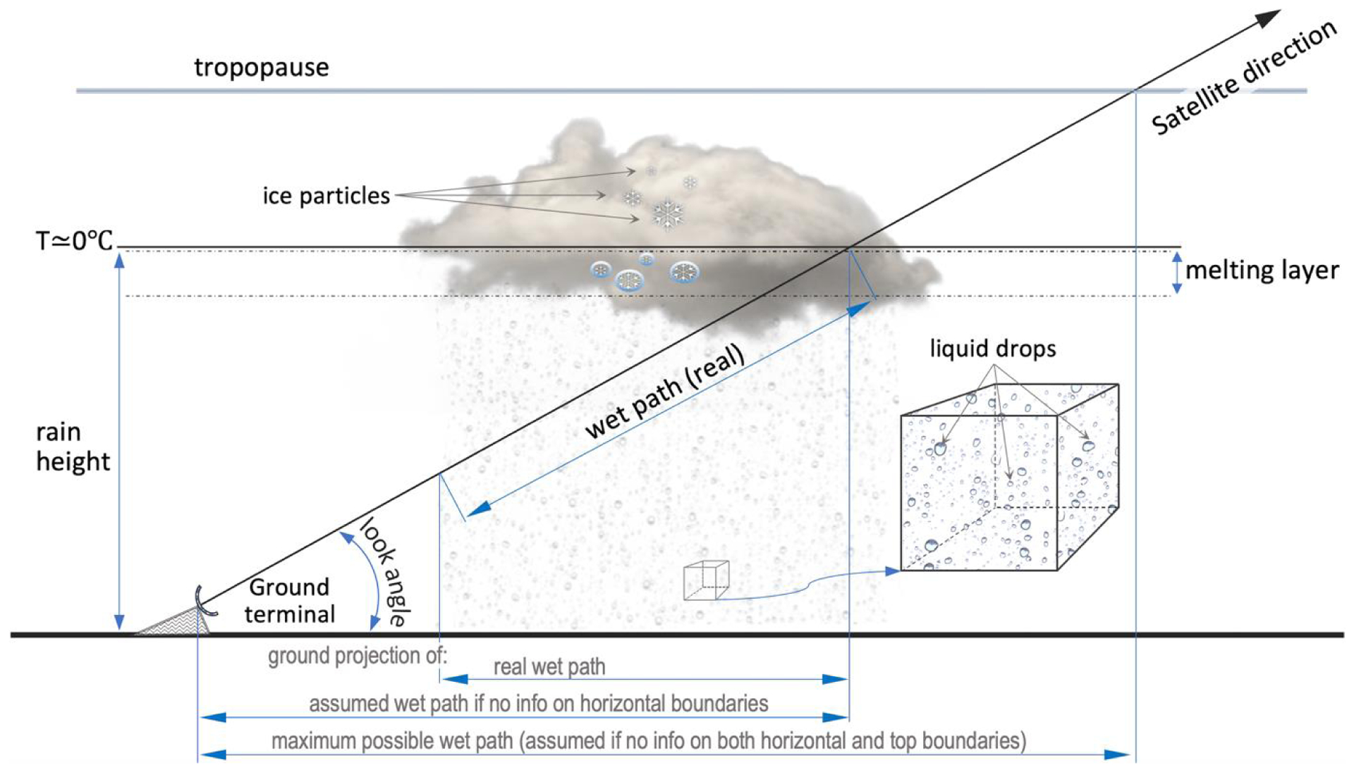
Schematics of the link geometry and segments contributing to the path attenuation.

Without information on the horizontal boundaries, we can only assume the same probability along the path: in this case, the rainfall integral is correct, but some spatial information is missed and intensity peaks are smoothed. In some cases, this information loss is negligible, namely when the ground projection of the wet path is much shorter than the horizontal scale of the rainfall system: this usually happens for very high look angles (70° or more) and also for lower angles during synoptic scale phenomena, causing stratiform precipitation with moderate height and homogeneous rain over long horizontal scales (tens of kilometers). Where advantageous, horizontal boundaries could be estimated, for instance from satellite observations.

Managing the lack of vertical information, i.e. top boundary, is more critical: when the path crosses the rain top before the tropopause (as normally happens), if rain fade is associated to the maximum path, we underestimate the actual integral rainfall over the horizontal projection of such a long path. Estimating the height of the rain layer and its uncertainty is thus necessary; it can be assumed to coincide with 0°C isotherm, taken from climatological data or, better, from operational weather simulations or ideally from local soundings, if available. Alternatively, it can be associated to the melting layer estimated from the bright band of weather radars.

Local intense convective precipitation events are expected to be the most problematic case, as they exhibit rapidly changing structures, with a small horizontal development, but a high vertical one, no more simply relatable to the 0°C isotherm.

Another issue is that melting drops have a different (typically augmented) effect on signal attenuation with respect to liquid drops with the same water mass, so that specific relationships for the attenuation should be assumed for the part of the wet path crossing the melting layer. Signal attenuation may be partially caused also by water on antenna reflector, radome, or feed horn, contributing up to several percentages to the measured attenuation (Blevis, 1965).

All these aspects should be considered when addressing the rainfall retrieval problem, or at least errors associated to these approximations should be evaluated and included in the measurement process.

Other sources of errors in the rainfall retrieval process are related to non-weather processes (Giannetti 2018). Instabilities on the emitting or receiving devices can cause such variations, and also the continuous slow drift of a geostationary satellite from its assigned position and its periodic (faster) repositioning. When attenuation is measured using some quantities related to S/N (signal to noise ratio), even an increase of noise due to artificial or natural causes (e.g. sun blinding of receiving antennas close to equinoxes) can be misinterpreted as rain fade. To cope with these issues satellite-dependent variations can be recognized and properly accounted, simultaneously processing data from a number of receivers far enough to be weather-uncorrelated; some local non-weather increase of noise can be fixed thanks to ancillary information and measures can be rejected, if necessary. Some non-weather variations have different signatures than rain-fade ones, and this enables the implementation of algorithms to filter them out to reduce the error. The contribution of these phenomena to the retrieval performance is still matter of research and it involves field experiments, that are not in the scope of this work. A thorough analysis of the impact on single receiver rain retrieval of different error sources, such as characteristics and variability of melting layer, and drop size distribution, has been conducted using coincident raingauge, weather radar and disdrometer measurements (Adirosi et al. 2020).

So far, we have referred to satellite links, but rain fade affects also terrestrial point-to-point microwave backhaul links and can be therefore used to measure rainfall along their paths (Overeem et al., 2016a; Messer, 2018), on the basis of the same concepts and with similar problems, except for satellite-specific issues and the rain height estimation, not affecting the wet path in terrestrial links.

In any case they all are instruments not conceived to measure rainfall and the only reason why the attenuation is monitored is because telecommunication companies have to guarantee a fully functional operational service even during precipitation, avoiding that rain showers attenuate the signals down to a S/N value so low to cause the outage of the radio link between transmitter and receiver. No obvious solutions exist to cope with this problem, because lowering the transmission frequency, besides ending up into a dramatically crowded radio-frequency spectrum, means also reducing the bandwidth and thus the information that can be carried, while increasing the emission power means rising the overall system costs. Cost-benefits analyses drive the technical requirements to achieve the optimal compromise for telecom companies, and not always they match meteorologists’ needs: in a given percentage of rainy events, telecom companies accept that rainfall intensity and extension cause the outage of the connection, but it also means that we cannot rely on such infrastructure to monitor very heavy rains. However, even a link outage condition does still provide some information: actually, it says that rainfall is heavier than a given threshold. Depending on the type of measured signal and of receive equipment, such a threshold ranges from 20 to 100 mm h⁻¹ approximately (Giannetti 2017, Giro 2020).

In the following we approach rain fade measurements from a network perspective to exploit the information contained in wet path attenuations and signal outages.

3. Rainfall fields reconstruction

The availability of measurements from different sources is a great perspective to retrieve rainfall fields. While radar and satellites give a spatial estimation of rainfall, in situ measurements need to be interpolated. For rain gauges, this task is accomplished via different techniques, from the simplest Thiessen polygons to sophisticated geostatistical techniques such as kriging with its variants (Webster and Oliver, 2007). Several complex aspects need to be considered in order to correctly estimate the relationship between areal and point rainfall, which depends on time scales and precipitation characteristics (Breinl et al., 2020). If applied to measurements from satellite or terrestrial microwave links, these techniques require certain adaptation. In fact, signal attenuation is associated with the presence of rainfall in a link path rather than in a specific point. So, the measurement is: i) indirect, ii) anisotropic and iii) integrated over a path. The spatial distribution of links also follows patterns that are driven by commercial rather than geophysical reasons (they are for example denser in urban areas), leading to an uneven distribution of data-void regions. On the other hand, the spatial density of instruments in certain areas can be very high compared to the one usually adopted for gauges.

These considerations in broad terms apply both to satellite links and to cellular networks. Various studies have addressed the task of the reconstruction of spatial fields from sparse MW links attenuation measurements. Overeem et al. (2016b) have done a thorough work producing maps for the territory of the Netherlands for two and a half years from an operational cellular network (~2,400 links), as a first attempt towards an operational application at large scale. They apply ordinary kriging interpolation with a climatological spherical variogram, associating the path averaged measurements to the center of the link segment. Several time scales have been investigated (from 15 minutes to 1 month), as well as different spatial scales. The obtained maps show a good agreement with the gauge-adjusted radar data albeit problems may arise in the estimation of the variogram for different time scales.

Attempts to merge rainfall estimations from multiple instruments are presented in Haese et al. (2017). They use a stochastic approach called random mixing to generate precipitation fields from a set of rain gauge observations and path-averaged rain rates estimated using commercial Microwave Links. They apply their method to both synthetic (generated via COSMO model) and real data in a study area in Germany, adopting a hourly time step.

Bianchi et al. (2013) also present a technique to combine measurements from rain gauges, weather radars, and telecommunication links. They apply a variational assimilation method with 5 minutes resolution, using rain rate from C-band radar as background state estimate and updating the estimation with 13 rain gauge measurements and attenuation from 14 cellular microwave links.

The above mentioned methods are strictly dependent on the availability of observations; when no measurement is available (or when the number of observations is not adequate) rainfall maps cannot be updated. This is especially relevant if a very fine time step (e.g. less than 5-minute) of analysis is required. Also, the accuracy in data-void regions can be poor.

A possible approach to overcome these limits is to use a spatio-temporal modeling framework combining the information from the link measurements with a dynamic rainfall advection model (assuming that during very short time intervals this can be representative of the storm evolution). Data assimilation techniques can then be used to optimally merge the information contained in the observations with those from the dynamic model.

Zinevich et al. (2009) follow this type of approach using an Extended Kalman Filter for the reconstruction of rainfall spatial-temporal dynamics from a standard wireless microwave network for cellular communications (23 links). They obtain near-surface rainfall maps at the temporal resolution of 1-minute. The results are validated using 5 rain gauge measurements and compared with other spatial interpolation techniques.

Mercier et al. (2015) propose a similar framework but their study differs from the one by Zinevich et al. (2009) for two major aspects of the data retrieval and processing: they use a 4D variational data assimilation scheme instead of Extended Kalman Filter and apply their procedure to broadcast TV satellite links instead of cellular communication networks.

In Zinevich et al. (2009) the direction of motion of the rainfall field is recovered from the simultaneous observation of a multitude of microwave links. For cellular networks this is possible thanks to the high number of links in different directions. The application to satellite links is more complicated since all links in a given system share the same viewing direction (they point to the same satellite, or at least to a limited number of satellites simultaneously). Mercier et al. (2015) use a Ku receiver capable of pointing to 4 different satellites, and need to rely on advection velocity retrieved from consecutive radar images. This might limit the applicability of the method in certain areas.

The data assimilation framework introduced in this paper is specifically conceived for an operational implementation; for this reason, several aspects have driven its definition. First of all, the formulation has to be computationally efficient and suitable for real time applications. The EnKF is particularly appropriate for this scope. Furthermore, the physical model is formulated in a way that it can ingest forcing data from available products of geostationary satellites. Finally, the peculiar errors discussed in Section 2 are taken into account.

The formulation is 3-dimensional so that it can take into account the vertical extent of the link path in case of broadcast satellite measurements. Figure 2 shows the flow path of the system. Starting from a first-guess state that can be obtained from real-time satellite rainfall products, the desired state (rain rate) is obtained through an EnKF data assimilation system where the rainfall field is predicted by an advection model and “corrected” on the basis of the available signal attenuation measurements.

Figure 2.

Flow chart of the proposed EnKF data assimilation scheme for the retrieval of rainfall fields at high temporal and spatial resolution from telecommunication satellite links. The box of the cloud boundaries, input for horizontal boundaries, is in faint colors with its link in dashed line because included in the concept but still not implemented in the algorithm.

Ancillary data are used for forcing (Atmospheric Motion Vectors, AMV) and for boundary conditions (rain rate estimates at larger scale from meteorological satellites).

4. Ensemble Kalman Filter formulation

Among data assimilation techniques, Kalman Filter (KF) has gained relevance for operational applications in different fields (from oceanography and meteorology to system control and signal processing) due to its suitability for real time usage and its relative simplicity of implementation.

The general form of the KF includes a “forecast step” (also called prediction step or prior estimate) where the state of the system at time t is estimated from the state at previous time step t − 1 by means of a dynamical model, and an “analysis” (or update) step where such state estimate is corrected comparing it with observations that can be either the same type as the state (e.g., rainfall rate), or a quantity that indirectly brings information related to the state (e.g., radiances). The observations and the state are connected through a measurement operator. Both model and measurement processes are uncertain, and the error information is propagated by means of the state error covariance matrix. The standard KF can be applied only when both the state evolution model and the observation operator are linear and errors are Gaussian. In such (ideal) case, the KF represents the optimal state estimator (Gelb, 1974).

The Ensemble Kalman Filter, EnKF (Evensen, 2003) is a Monte Carlo approach that can be used to overcome the strong operational limitations of the standard KF, namely i) the non-linearity of many dynamical systems and ii) the high computational effort required for the storage and forward integration of the forecast error covariance in large systems. In the EnKF, the covariance is estimated from the generation of an ensemble (statistical sample) of state replications. The EnKF has proved to be a robust estimator even in presence of deviation from Gaussianity assumption (Katzfuss et al. 2016). Many successful applications of EnKF have been used to assimilate various types of observations into atmospheric and land surface models (Reichle et al., 2002, De Lannoy and Reichle, 2016).

Different variants of the EnKF have been proposed (Houtekamer and Zhang, 2016). One of the main splits is between the so-called “stochastic” and the “deterministic” EnKF. In the former the observations, as well as the states, are treated as random variables and an ensemble of observations is generated around the actual measured values (Burgers, 1998, Houtekamer and Mitchell, 1998). Instead, the methods that fall into the “deterministic EnKF” category avoid the randomization of observations and propagate an ensemble of deviations from the ensemble mean (Sakov and Oke, 2008; Roth et al. 2017).

In the present study, the stochastic EnKF approach is chosen because it allows us to formulate a particular structure of the observation error.

The specific forms of the different components of the data assimilation framework are described below.

a). State-space formulation

The spatial domain is depicted by a computational Cartesian 3D grid with D_y rows, D_X columns and D_z vertical levels, then a total number of elements n = D_x · D_y · D_z. Grid step Δg is set equal in all three dimensions.

Indicating with r_ijk, the rain rates in mm h⁻¹ in the cell (i, j, k) of the domain, we define the transformed variable x at time t as:

$$x_t={\left[\text{log}\left(r_{111}+\epsilon \right),\dots ,\text{log}\left(r_{ijk}+\epsilon \right),\dots ,\text{log}\left(r_{D_y{D}_x{D}_z}+\epsilon \right)\right]}_{\text{t}},$$ (1)

where ε is a small positive number (set to 10⁻⁶) that ensures a finite value when r = 0. It is merely a numerical artifact and is omitted for simplicity in the continuing of this paper.

The use of a logarithmic variable is established in order to preserve non negativity. Janjic et al. (2014) have analyzed several precautions and drawbacks that need to be considered when using this approach in an EnKF formulation. For example, particular attention must be put in the choice of an appropriate error covariance.

b). Forward (advection) model

At each time step the rain rate in the cells of the domain is propagated forward step by means of a dynamic state transition model F.

Since the model is not perfect, it has an associated error ω_t so that the state at time t is predicted from the state at previous time step as:

$$x_t=F_t\left(x_{t-1}\right)+{\omega }_t.$$ (2)

The simplest form of F is considering a very basic advection model where the precipitation field moves horizontally by means of the East-West (u) and North-South (v) wind components.

In this case F can be easily built in the spatial domain (mesh of the D_x · D_y · D_z cells): in the non-transformed space (considering the rain rate r instead of x = log(r)), F can take a linear form represented by a sparse state transition matrix F_t where the non-zero elements are conveniently placed so that the rain rate which at time t is in cell i,j,k, will shift at time t + 1 in the x and y direction respectively with:

${\left(\Delta x\right)}_{ijk,t}=\frac{u_{ijk,t}\cdot \Delta t}{\Delta g}$ and ${\left(\Delta y\right)}_{ijk,t}=\frac{v_{ijk,t}\cdot \Delta t}{\Delta g}$, with u_ijk and v_ijk being the East-West and North-South wind components in the i,j,k element at time t. Time step and grid size need to be accordingly chosen for numerical stability.

Rain rates at time t are then advanced as r_t = F_tr_t−1. When applying the logarithmic transformation, the system is no longer linear since, after some straightforward arrangements, we write:

$$x_t=\text{log}\left(F_t\text{ exp}\left(x_{t-1}\right)\right)+{\omega }_t.$$ (3)

In an operational context, wind velocities can be obtained from AMV satellite products that are routinely produced and disseminated by several agencies worldwide (Santek et al., 2019). AMV are retrieved from the apparent motion of coherent features tracked in consecutive images from geostationary satellites, assuming that this is representative of the wind at a certain height in the atmosphere. (Lean et al., 2015).

Boundary conditions are also derived from satellite products. In this case the instantaneous rain rate provided from infrared or blended infrared/MW satellites can be used.

The model error term ω_t ~ N(0, Q_t) is a white, Gaussian sequence with Q_t a (n × n) symmetric positive definite covariance matrix. ω_t incorporates all the errors related to the formulation of the advection model and also the uncertainties in the forcing data. In case of spatially uncorrelated error, Q_t is diagonal; in the present case it is assumed instead that spatial correlation exists within a certain distance. This reflects the fact that neighboring cells are likely prone to the same error sources in terms of forcing data and also considers the autocorrelation of rainfall fields, that at very short time scales can be assumed at most a few kilometers (Villarini et al., 2008). So, Q_t is expressed as Q_t = q · L where q is a constant value (representative of model error variance) and L is a correlation matrix built from Euclidean distances between cells. Several distance functions can be used: their general requirements are to be positive-definite and to guarantee an adequate smoothness. A commonly used function is the 5^th order compactly supported function (Gaspari and Cohn, 1999), which is similar to a Gaussian in shape but with correlations decreased to zero at a finite radius.

It is instead assumed that ω is uncorrelated in time.

c). Ensemble

Following a Monte Carlo approach as expected in the EnKF, N statistical samples of the initial state are generated: this can be accomplished, for instance, perturbing an initial guess x₀ with the model error ω so that the i-th ensemble is:

$${x_0}^{\left(\text{i}\right)}=x_0+{\omega }_0^{\left(\text{i}\right)}i=1\dots N.$$ (4)

The advection model is applied for each ensemble member:

$${x_t}^{\left(\text{i}\right),\text{f}}=F_{\text{t}}\left(x_{t-1}^{\left(\text{i}\right)}\right)+{\omega }_{\text{t}}^{\left(\text{i}\right)}.$$ (5)

The superscript f stands for “forecast” (as opposed to “analysis”).

The main limitation of ensemble size is the computational burden. For operational application at basin or regional scale, it is expected that the size of the state vector (number of cells in the spatial domain) is likely to reach O(10⁶). Although increasingly powerful resources are available, and appropriate methodologies can be used to optimize the computation (i.e. sequential processing of batches of observations), for a real-case application the allowed ensemble size will hardly exceed O(10³).

d). Observations

At time step t a certain number of rain rate estimations m_t from broadcast signals is available, so that a vector of observations z_t can be constructed.

The number of available observations can be different at each time step (due to instruments that are out of service or provide data at different time steps). If no data is available, the analysis step is omitted and the state estimate is set equal to the ensemble mean of the forecast. The observations are related to the state variable x_t so that:

$$z_t=H_t\left(x_t\right)+v_t,$$ (6)

where H_t is a measurement operator that projects the state space onto the measurement space and υ_t is the measurement error that reflects the uncertainties in the measurement process (later discussed). If the observed variable is the rain rate calculated from signal attenuation, H_t serves to geometrically identify the grid elements that lay within the wet path at time-step t. Given the position and viewing direction of the ground terminals and the estimated precipitation height, for each GT observation the indices of the cells in the 3D matrix that are crossed by the wet path are identified (a cell is tagged as belonging to the wet path regardless of portion of cell crossed). We can therefore build a sparse (m_t × n) matrix H_t with non-zero elements along the path, which multiplied by the n-dimensional state vector with the rain rates at time t (to be precise by the exponential of the state vector containing the logarithmic rain-rate values), entails to sum up the contributions of the cells in the wet path. We assume that each portion of the path contributes equally to the attenuation, so H_t produces the average rain rates equally weighting the contribution of each cell crossed by the path, i.e. the value assigned to the non-zero matrix cells is 1/(number of cells in the specific wet path). Although the link trajectory is fixed, H_t can vary at each time step depending on precipitation height, as discussed in Section 2.

If other approaches are followed (i.e. assimilating the raw attenuation data), H takes a more complicated form because the measurement operator needs to incorporate the algorithms for attenuation-rain rate inversion. This is possible in EnKF because it does to require linearity. It is also possible to do the full analysis in attenuation space, and convert to rain rates in post-processing phase.

Following a stochastic formulation of the EnKF, observations are also treated as random values and perturbed observations are generated at each time step, peculiar to each ensemble member, adding a random realization of the measurement error, so that:

$$z_t^{\left(\text{i}\right)}=z_t^o+v_t^{\left(\text{i}\right)}i=1\dots ,N,$$ (7)

with $z_t^o$ is the set of actual observations at time t and υ_t is the measurement error. The structure of υ_t is particularly challenging in the present formulation. In fact, under general conditions υ_t can be assumed normally distributed ~ N(0, R_t) where R_t is the measurement covariance (related to the instrument error). R_t is here set diagonal, meaning that we assume that the measurement error is not spatially correlated.

In the case of rainfall estimation from signal attenuation, we have already pointed out (Section 2) that links outages occur for heavy rains above a threshold value that depends on the characteristics of the signal and the GT. For this reason, when the estimated rain rate is at threshold value, υ_t is drawn from a skewed normal distribution (Azzalini and Capitanio, 1999), with parameters that can be tuned depending on the rain event.

e). Analysis step

In the update step of the Kalman filter, each ensemble member state is “corrected” on the basis of the misfit between the predicted value and the observations.

The update is performed multiplying the innovation vector (actual observation minus predicted value) by a gain term. The update state in EnKF is applied to each ensemble member obtaining the analysis states:

$$x_t^{\left(\text{i}\right),\text{a}}=x_t^{\left(\text{i}\right),\text{f}}+K_t\left(z_t^{\left(\text{i}\right)}-H_t\left(x_t^{\left(\text{i}\right),\text{f}}\right)\right).$$ (8)

The Kalman gain matrix K_t in EnKF formulations can be estimated in slightly different ways. A discussion on various approaches for calculating and interpreting optimal Kalman gain, especially in the case of nonlinear measurement operators can be found in Tang et al., 2014. Following Houtekamer and Mitchell, 2001 we calculate K at time t as:

$${\text{K}}_{\text{t}}={\text{P}}_{\text{xy},\text{t}}{\left({\text{P}}_{\text{yy},\text{t}}+{\text{R}}_{\text{t}}\right)}^{-1},$$ (9)

where P_yy,t is the error covariance of the measurement predictions and P_xy,t is the cross covariance between the state and the measurement predictions.

Once all the ensemble members are updated, we calculate the ensemble mean and assume such value as the actual state estimate at time t, $\widehat{x_t}$ (and consequently rain rate $\widehat{r_t}=\text{exp}\left(\widehat{x_t}\right)$):

$$\widehat{x_t}=\frac{1}{N}{\sum }_{i=1}^N{x}_t^{\left(\text{i}\right),\text{a}}.$$ (10)

5. Synthetic experiments

5.1. Experiment setup

The data assimilation system has been applied to a small spatial domain as a test-bed where a set of synthetic experiments has been performed. The aim of the synthetic experiments is to evaluate the feasibility of the method and tune up its different components. They also serve to estimate the computational burden of the procedure and define operational strategies.

The domain is a gridded area with 30 rows, 30 columns and 10 vertical levels. Cell size is 500 m in each direction. It represents therefore a spatial domain of 15×15 km² that extends in the vertical up to 5 km, and the state vector is composed by 30×30×10 = 9000 rain rate values. Time step of analysis is 1-minute. This is both the step of the forecast advection model and the update of the observations.

A set of simulated 3-D rainfall fields has been generated: the “true” rainfall field has a simplified cylindrical shape with higher intensity in the center (max rain rate = 60 mm h⁻¹) and decreasing intensities up to a radius of 6 km (rain rates higher than 20 mm h⁻¹ are concentrated in a radius of about 2 km). Rain rate is constant in the vertical from the ground to a rain height of 4 km. This spatial structure is assumed to move horizontally with a certain advection velocity. The use of geometrically-shaped rainfall systems must not mislead: neither the sampling nor the EnKF procedures exhibit any particular symmetry that could facilitate the reconstruction of geometric shapes. They are of course unrealistic, but by no means easier to retrieve; conversely, they facilitate the detection and interpretation of the differences with the reconstructed precipitation shapes.

Realistic forcing and auxiliary data are also simulated. Initial conditions and lateral flux entering the domain are derived mimicking the observations from a geostationary satellite such as MSG or GOES. These data are built degrading the “real” synthetic initial state to a spatial resolution of 3×3 km² and adding inaccuracy by means of: i) misplacement error (shifted position with respect to the “real” conditions) and ii) random additive error. A first-guess rain height is also set. Boundary conditions are assumed to be available every 5 minutes (like, for example, MSG rapid scan products), and they are kept static in the period between updates: this is another source of error. AMV are assumed constant over the spatial domain and their value is guessed with multiplicative and/or additive errors to the u and v components of the “real” storm. Again, in order to mimic the availability of data in an operational context, we assume that new AMV are available every 20 minutes.

Finally, 80 ground terminals (GT) for broadcast satellite signal reception are placed in randomly selected locations in the study area. Although not relevant since we are dealing with synthetic rainfall fields, geographic coordinates have been assigned in order to simulate a real setting, localizing the study area over the city of Florence, Italy, and the terminals are directed towards two geostationary telecommunication satellites corresponding to EUTELSAT10 (placed at 10° E), and ASTRA 2F (placed at 28.2° E).

GT locations are drawn randomly without specifying any constraint (e.g. minimum distance between devices); this is done in order to represent a realistic situation where the observation network is not specifically designed for rainfall estimation. For this reason, links may nearly overlap in certain areas and be sparse in others.

Link paths are geometrically reconstructed from the satellite positions and elements of the 3D grid mesh have been tagged. Here we use links directed towards two specific satellites, but the methodology can be applied to every combination of link path, including terrestrial cellular paths (horizontal links). The interplay between the space-time variability of rainfall and the spatial geometry of the sensor network is expected to impact on some extent on the quality of the retrieved rainfall fields. Several experiments were performed from the beginning of this work to investigate this potential issue, playing with different angles between the observing devices and the synthetic rainfall paths, but we found no critical dependencies, apart from some expected differences on the domain boundaries and minor effects on the timeliness in reconstructing the shape of the precipitation system in the retrieval process. Part of such investigation is however shown through the experiments presented in the paper differentiated by different origins and track directions of the precipitation fields (see Section 5.2), so that the observations taken at the GT have the aforementioned minor variations in the timeliness and capabilities of detection.

In order to generate the synthetic observations, at each time step the signal attenuation is calculated from the rain in the cells belonging to the wet path. A power law relation between specific attenuation (dB km⁻¹) and rain rate (mm h⁻¹) is assumed, with parameters derived for Ku frequencies by Giannetti et al. (2017) from six years of disdrometers data taken in Rome, Italy. Measurement errors are introduced assuming a wrong estimation of precipitation height (in the range ± 500 m of error for the freezing level height): this implies that the attenuation sensed at a GT is assigned to a wet path a little different from the real one, thus affecting rain rate estimation associated to such sensor. Additional errors are generated adding Gaussian noise to the measurements (with 2 mm h⁻¹ standard deviation). Furthermore, when the estimated rain rate exceeds 40 mm h⁻¹, the value is cut-off in order to simulate the signal saturation effect (i.e. link outage). These assumptions allowed to reconstruct plausible synthetic observations, but of course various complex mechanisms may actually contribute to measurement errors (see Section 2) and, since rainfall estimation from telecommunication links is not a standard procedure, different devices and algorithms will lead to estimates with partially different error structures. The synthetic observations produced for this study are clearly a simplified approach, and careful considerations need to be taken when dealing with real data.

5.2. Results

The experiments have been performed for a wide range of conditions, changing storm velocities as well as boundary and initial conditions.

Figure 3 shows the results for a storm moving in South-East direction with constant velocity with u_true=5 m s⁻¹ (positive east) and v_true= −5 m s⁻¹ (positive north). In the first row, the maps of rain rate at ground level at selected time steps for a 20 minutes simulation are shown (for figure clearness results are shown every 3 minutes but time step of analysis is 1-minute). Second row shows the “openloop” (forward model without observations), derived assuming imperfect forcing data with AMV velocities of u_model = 3 m s⁻¹ (i.e. 0.6·u_true) and v_model = −6 m s⁻¹ (i.e. 1.2·v_true) and a flawed simulated initial condition (coarser resolution with misplacement and random error): due to the inaccurate advection velocities the openloop rainfall fields deviate from the true (synthetic) ones and show a different trajectory. Third row shows the map obtained using only rain rate estimations from signal attenuation and treating them as point observations (spatially interpolated with nearest neighbor). Here, the observation is assigned to the GT position, without any consideration on viewing angle and spatial representativeness. This is clearly a source of error; furthermore, underestimation occurs when the rain rate exceeds the threshold value of 40 mm h⁻¹. Note that the “Obs.only” values (in this figure and the following) are not, to be exact, the assimilated observations, since in the assimilation scheme the measurements are connected to the cells in the 3D link path (through the measurement operator H_t) and not solely to the point position of the GT. The “Obs.only” rainfall fields are therefore a baseline for comparison; smarter spatial interpolation techniques could lead to improved estimations.

Figure 3.

Rainfall fields at ground level in the study domain (15×15 km²) at different time steps (minutes). Images are shown every 3 min., but time step of the model is 1 min. Dots indicate the locations of the ground terminals. First row: true (synthetic) rain rate [mm h⁻¹]. The storm moves in S-E direction with wind speed components u_true = 5 m s⁻¹ and v_true = −5 m s⁻¹. Second row: rainfall fields obtained from the openloop model which has advection velocities of u_model = 3 m s⁻¹ and v_model = −6 m⁻¹ s and initial condition from simulated satellite rainfall products. Third row: rainfall fields obtained interpolating the (synthetic) rain rate estimations from broadcast satellite links (with nearest neighbor interpolation). Fourth row: rainfall fields obtained with the EnKF with N=100 ensembles. The cyan circle in rows 2,3,4 outlines the boundary of the true rainfall in order to show the correct placement of the precipitation field.

Finally, in the fourth row the maps obtained with EnKF are shown: it can be seen that the reconstructed fields are more consistent with the “true” (synthetic) ones in terms of shape, intensity and position.

This is also evident when considering the trajectories of the precipitation field centroids (Figure 4). Black line is the trajectory of the true storm. Blue line is the openloop and reflects the errors assigned to the forward model (misplaced initial condition, errors in advection velocity). Red line is the trajectory of rainfall fields obtained from the “Obs.only” spatial interpolation. In this case, the misfit is mainly due to the viewing geometry of the devices with respect to the direction of the storm. Finally, green line is the trajectory of the rainfall field obtained with the EnKF simulation: the trajectory is closest to the “true” one and the assimilation system is able to redirect the storm in the correct direction.

Figure 4.

Trajectories of centroids of the rainfall field at ground level. Lines: black = true; blue = openloop; red = from observations only (rain rate from signal attenuation, spatially interpolated with nearest neighbor), green = EnKF. Markers are placed every 5 minutes (but model time step is 1-minute). Also shown is the position of ground terminals (gray “hat” symbol ^) and satellite links (gray dotted lines) pointing to two broadcast satellites (the link path projection is shown up to the precipitation height of the experiment = 4 km).

The good estimation performed by the EnKF is assessable also evaluating error with a pixel-by pixel comparison. Figure 5 shows at each time step the Normalized Root Mean Squared Error (NRMSE) of rain rate estimation at ground level, calculated as RMSE of all the n_g pixels divided by their spatial mean:

$${\left(\text{NRMSE}\right)}_{\text{t}}=\frac{\sqrt{\frac{1}{n_g}{\sum }_{\text{j}=1}^{n_g}{\left(\widehat{{\text{r}}_{\text{j}}}-{\text{r}}_{\text{j}}^{\text{true}}\right)}_{\text{t}}^2}}{\frac{1}{n_g}\left({\sum }_{\text{j}=1}^{n_g}{\text{r}}_{\text{j}}^{\text{true}}\right)}.$$ (11)

Figure 5.

Normalized Root Mean Squared Error (NRMSE) of rain rate estimation at ground level calculated for each time step as RMSE divided by spatial mean of cell values. Blue = Openloop model; red = Observations only (spatially interpolated with nearest neighbor); green = EnKF (solid line = EnKF with 100 ensemble members, dashed-dot = EnKF with 50 ensemble members, dotted = EnKF with 500 ensemble members).

The NRMSE for EnKF (solid green line) is lower than both the openloop and the “Obs.only” estimation, and decreases with the progressing of the assimilation.

The same figure also shows the error obtained with the same experimental set-up but with a different number of ensemble members (green dashed and dash-dot lines). The issue of ensemble size is of prime importance for filter’s efficiency; in fact, a small ensemble can lead to wrong estimation but a high number of members requires high computational costs. The choice of optimal ensemble size is a balance between these two requirements and is related to the specific application (depending on state, number of assimilated observations, characteristics and uncertainties of the forward model). For the present experiments the results suggest that N=100 is satisfactory, since a higher number (N=500) leads to similar errors (on the contrary, N=50 gives poorer estimations). This is encouraging for the feasibility of the method, but further evaluation is needed when applied to larger domains with different configurations and real data.

Other synthetic experiments have been performed, with the same cylindrical storm but changing “true” and modeled advection velocities, obtaining similar outcomes. Detailed outputs are not presented in this paper but Figures 6 and 7 summarize some of them. The figures show (left panels) the trajectories of the centroids of precipitation fields at ground level for rainy systems moving in cardinal directions (E, W in Figure 6 and N, S in Figure 7) assuming various model errors. We can see that in any case the EnKF is able to correct for the wrong first-guess advection velocity. NRMSE error also decreases (right panels) for the EnKF with respect to the openloop and the “Obs.only”, taking advantage of both the model and the observations. The fact that the reconstruction of rainfall fields is satisfactory for all track directions, suggests that the methodology can deal with different reciprocal interactions between sensor network and precipitation patterns, with no criticalities. Further and more comprehensive investigations will be performed in future work with data from real networks, possibly of various type (broadcast satellites, cellular or combination of both).

Figure 6.

Summary of results for other synthetic storms in cardinal directions: a) trajectories of centroids of rainfall at ground level (same as figure 4); b) Normalized Root Mean Squared Error (same as figure 5 but only with EnKF with 100 ensemble members) for a storm moving eastward. c) and d) are the same as a) and b) but for a storm moving westward.

Figure 7.

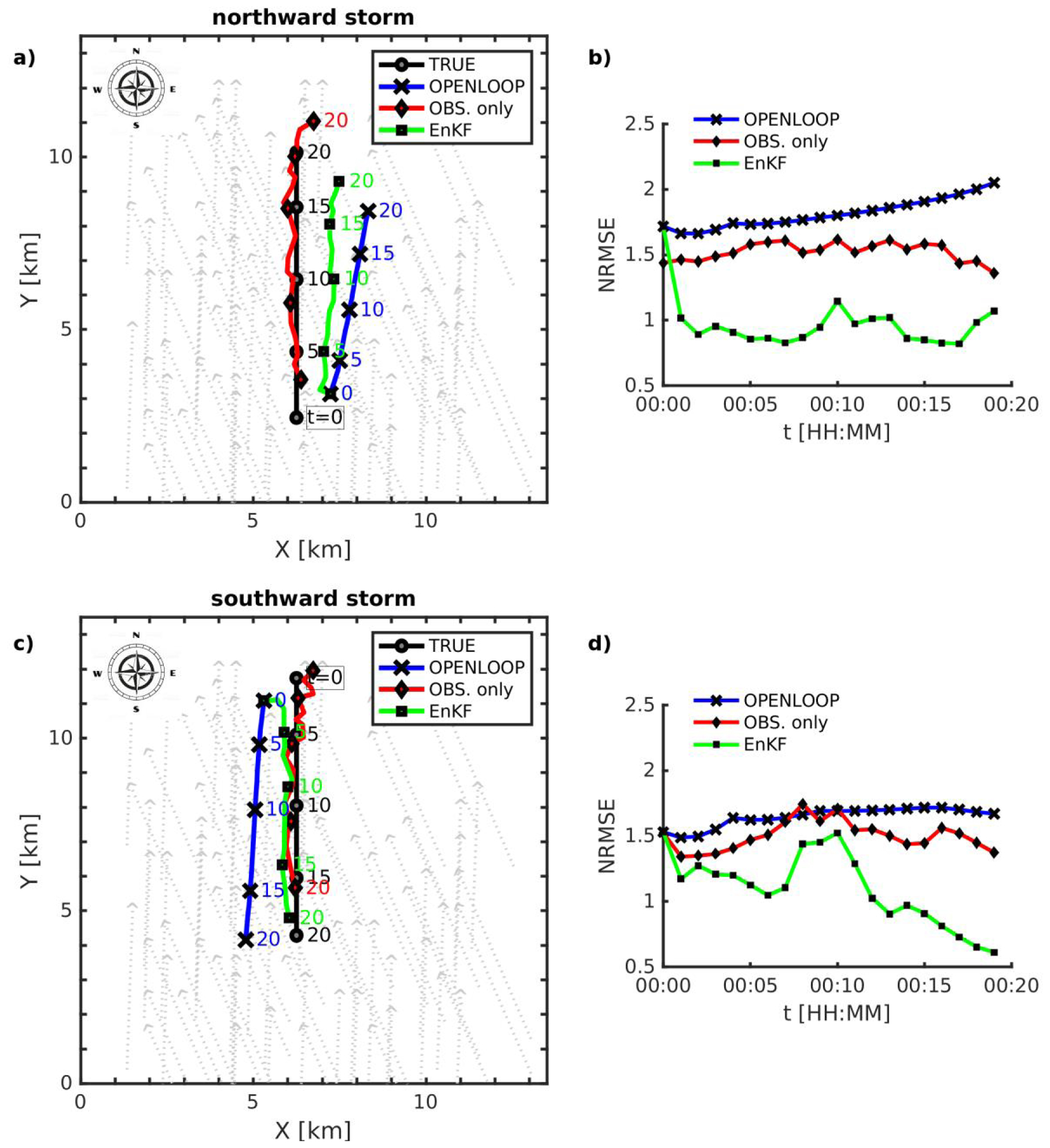
Same as figure 6 but a) and b) for a storm moving northward, and c) and d) for a storm moving southward.

NRMSE alone may not provide sufficient information on the model performance; for example, it does not discern the ability to reproduce high precipitation values or to detect rain/no rain areas. For a basic verification of the performance for various precipitation thresholds, several commonly used skill scores are reported in Table 1. For the calculation of scores, a hit is defined when a grid point exceeds a certain rainfall threshold both in the real (synthetic) rainfall field and in the EnKF; a false alarm is when a grid point exceeds the threshold in the EnKF rainfall field but not in the real one; a miss occurs when a grid point exceeds the threshold value in the true field but not in the EnKF.

Table 1.

Skill scores of the EnKF method (ability to detect rainfall above various thresholds).

Rainfall threshold	POD	FAR	TS	FBIAS
> 0.5 mm h−1	0.92	0.34	0.62	1.40
> 2.5 mm h−1	0.91	0.31	0.65	1.33
> 5 mm h−1	0.92	0.25	0.71	1.22
> 10 mm h−1	0.91	0.19	0.75	1.12
> 20 mm h−1	0.85	0.18	0.71	1.04
> 30 mm h−1	0.76	0.25	0.61	1.02

Statistics are calculated cumulatively for 8 synthetic experiments (cylindrical storms moving in N, W, S, E, NW, NE, SW, SE) with 20 minutes duration each, 1-minute time step, over a domain with 30×30 ground cells. POD (probability of detection) = hits/(hits + misses); FAR (false alarm ratio) = false alarms/(hits + false alarms); TS (threat score) = hits/(hits + misses + false alarms); FBIAS (frequency bias index) = (hits + false alarms)/(hits + misses).

Six rainfall thresholds are set, from 0.5 mm h⁻¹ to 30 mm h⁻¹. Scores are overall satisfactory for all thresholds, confirming the method goodness.

6. Experiment with real rainfall and forcing data

6.1. Experiment setup

In order to advance the evaluation of the model towards a more realistic scenario, we have set up a further experiment where the storm is derived from the reflectivity data from an X-band radar placed in Florence area. The VMI (Vertical Maximum Intensity) images taken on October 29^th 2018 from 0510 to 0520 UTC over the study area (same domain as the previous experiments) have been converted into rainfall rate using the standard Marshall-Palmer relationship (Marshall and Palmer, 1948), and resampled at 500 m spatial resolution. Rain height is 3 km.

AMV, first guess rainfall fields and boundary conditions are taken via the EUMETSAT Data Centre (AMV product and MPE product).

Attenuation measurements were instead retrieved again as synthetic observations, with same placement of links as in the previous experiments, since data from a homogeneous and sufficiently dense experimental network is not available yet.

This experiment is therefore still a synthetic one; however, it is useful because it allows to test the methodology with complex storm structures instead of idealized cylindrical storms and also to deal with uncertain forcing data whose error is not known.

6.2. Results

The simulation was performed again at 1-minute time step. Figure 8 (analogous to Figure 3) shows the maps of rain rate at ground level at selected time steps for the 10 minutes simulation. For figure clearness results are shown every 2 minutes. The initial rainfall field and the openloop model do not show the correct spatial patterns and dynamics, probably due to coarser resolution and temporal sampling of 5 minutes of MSG data, while the “Obs.only” maps exhibit the same inaccuracies of the previous experiment in terms of spatial representativeness and maximum retrieved rain rate. Instead the EnKF (last row), that sequentially assimilates the (synthetic) rain rate observations from satellite links, after a few time steps produces rainfall fields that are consistent with the true ones. In particular, areas with higher rain intensities are located with sufficient precision, as shown also in Figure 9 with the 5-minutes cumulated rainfall fields from 0515 to 0520 UTC.

Figure 8.

Rainfall fields at ground level in the study domain (15×15 km²) at different time steps for a synthetic experiment based on real data. Images are shown every 2 minutes, but time step of the model is 1-minute. Dots indicate the locations of the ground terminals. First row: true rain rate [mm h⁻¹], derived applying the Marshall-Palmer formula to VMI values of a X-band radar from 0510 to 0520 UTC on 29/10/2018. Second row: rainfall fields obtained from the openloop model which has advection velocities (AMV) and first guess rain rate from EUMETSAT MSG satellite products. Third row: rainfall fields obtained interpolating the (synthetic) rain rate estimations from broadcast satellite links (with simple nearest neighbor interpolation). Fourth row: rainfall fields obtained with the EnKF with N=100 ensembles. The cyan outline in rows 2,3,4 marks the boundary of the true rainfall in order to show the correct placement of the precipitation field.

Figure 9.

5-minutes cumulated rainfall (from 0515 am to 0520 UTC of 29/10/2018) in the study area (15×15 km²). True is on the left, OBS.only is in the center and EnKF is on the right.

The good model performance that can be visually appreciated in Figures 8–9 is confirmed by the scatterplots of true rain rate at ground level in each pixel versus the values obtained from the EnKF procedure (Figure 10). Correlation coefficients and NRMSE are also shown.

Figure 10.

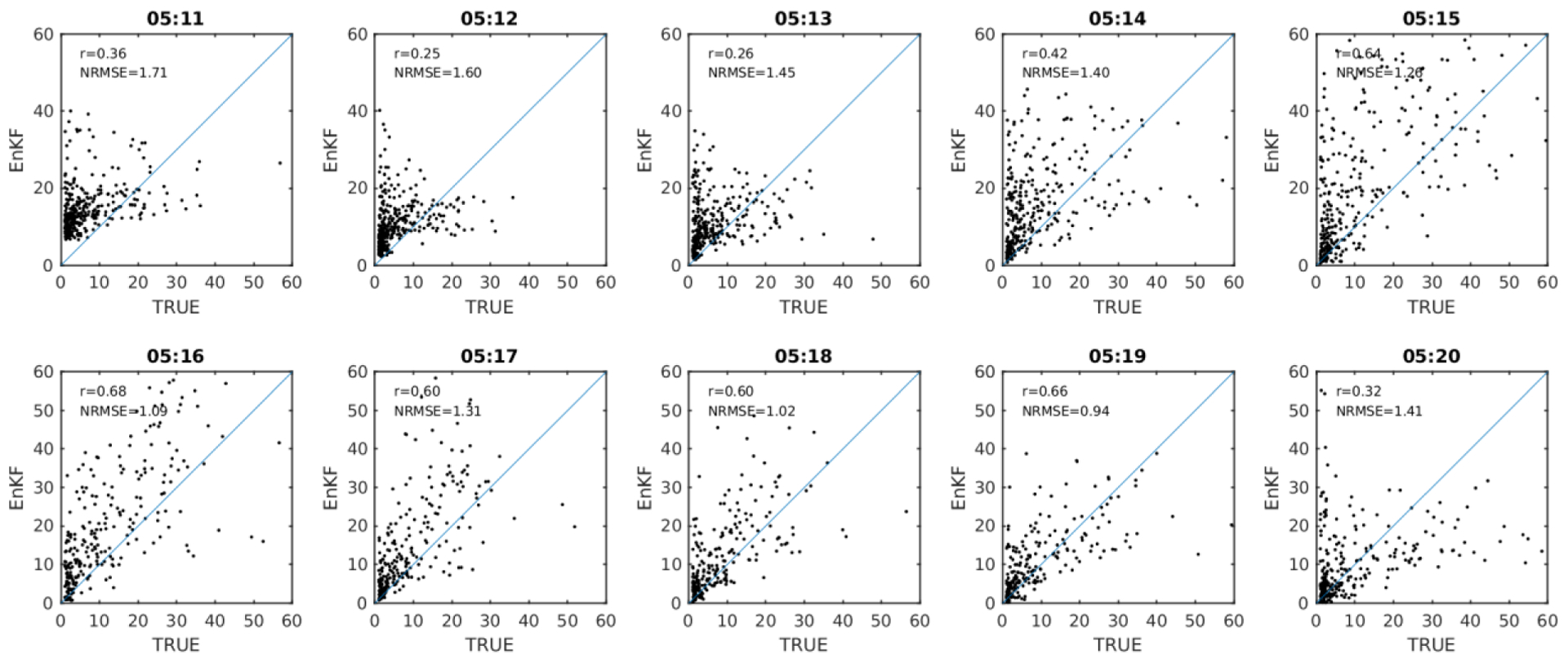
Scatterplots with comparison on a pixel-by-pixels basis of true rain rates at ground level (from X-band radar) versus those estimated with EnKF procedure. Correlation coefficients and NRMSE are also shown.

Finally, for a point-specific evaluation, we have extracted the time series of precipitation in selected pixels of the domain at ground level (Figure 11). Both for point A (interested by the transition of rainfall with high intensities) and for point B (with lower rain rates), the estimation obtained with the EnKF is more accurate with respect to the openloop based on MSG data only (that gives a near constant value in the study interval) and also with respect to the “Obs.only” approach. In point A the “Obs.only” rain rate is underestimated, due to link outage (rain rates higher than 40 mm h⁻¹ are not detected) and to the distribution of rainfall in the path, while in point B rain rate is overestimated, probably due to the interception of rainfall that is on the link path but not on the GT position.

Figure 11.

True (from X-band radar) and estimated hyetographs at two sample points A and B.

As a further demonstration of the methodology, comparable results have been obtained for another rainfall period occurred later on the same day, from 1500 to 1510 UTC. Figure 12, analogous to Figure 8, shows the “true” rainfall fields (from radar) at different time steps, those obtained from the openloop model (that in this case underestimates the rain rates), the “Obs.only” and the EnKF, which again produces rainfall fields with patterns and values consistent with the true ones.

Figure 12.

Same as Figure 8, but for the period from 1500 to 1510 UTC on 29/10/2018.

As for the synthetic experiments described in Section 5, the skill scores have been calculated for six rain rate thresholds. The results are good apart from a slight tendency to overestimate the high precipitation values (increasing false alarm ratio and bias score for moderate and heavy rain). We remind that rainfall rate from MW links are upper limited and probably this small overestimation is due to something improvable in the statistical model assumed for rainfalls greater than such limit.

Since the synthetic events reconstructed from radar are not simplistic as the cylindrical shapes, it is also interesting to evaluate if the statistical distributions of the “true” and simulated rainfall fields exhibit the expected analogies. In the boxplot of Figure 13, the two distributions appear very consistent, apart from the slight tendency to overestimate the high precipitation values discussed above.

Figure 13.

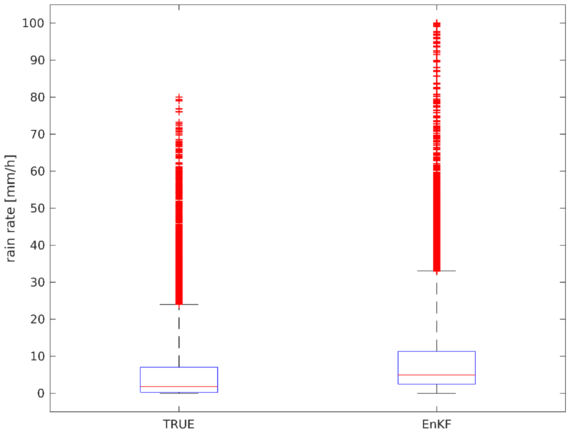
Boxplots of the “true” rain rate distribution (all grid points in the domain for all time steps) and the one reconstructed with the EnKF. The box margins indicate the 25^th and 75^th percentile, while the whiskers indicate the 5^th and 95^th percentile.

7. Summary and Conclusions

In this paper several aspects related to rainfall measurements from telecommunication MW links, especially in the case of satellite links, have been analyzed.

These data require a number of uncertain assumptions and ancillary information, because of observation geometry and specific technique, and the information they carry have a probabilistic nature due to errors associated with non-weather phenomena, link outage during heavy rains, and the intrinsic path-averaged nature of the measurements. Direct comparisons with rain gauges can be useful for an initial understanding of relationships and uncertainties, but looking at these measurements as rain gauge surrogates, and then spatialize them in some way, is not the right way to proceed. Therefore, we have designed a framework to dynamically generate homogeneously-gridded rainfall fields, assimilating precipitation from MW links through an EnKF approach. Tests are made through synthetic 3D experiments, with increasing proximity to realistic cases, i.e. from purely geometric storms to phenomena built from weather radar and satellite observations. Ancillary data, available from meteorological operational satellites, are used for advection information and initial and boundary conditions. Rain height is assumed as estimated from high-resolution operational meteorological models. The method is flexible, applicable to different observation geometries and characteristics. A small set of experiments is reported among the several ones performed with different errors, link outage thresholds, geometries, number of sensors, rainfall structures, ensemble members, to demonstrate its feasibility. The method correctly reproduces rainfall structure and quantities and is practicable also in operational contexts from the point of view of the computational burden. On the basis of the simulations performed on a small domain and some scale up tests, we estimate that a regional domain approximately of 100×100 km² could be run operationally, with the same characteristics of our experiments, using a server and an optimized code (i.e. one-minute analysis steps would need less than one-minute of computing time).

The next step is to move to the use of only real measurements. This implies to deepen the error analysis, including the specific ones from meteorological satellite products used as forcing. The team is involved in initiatives experimenting operational set-up for rainfall retrieval from satellite links, and this will give the opportunity to improve the measurement performances and the error characterization. We believe that these studies are worth to be done, given the wide demand of accurate rainfall information at very high spatial and temporal scales, and that MW links, if properly managed, could have a relevant role in this challenge.

Table 2.

Skill scores of the EnKF method (ability to detect rainfall above various thresholds) for the experiments described in Section 6 (precipitation fields from radar).

Rainfall threshold	POD	FAR	TS	FBIAS
> 0.5 mm h−1	0.95	0.32	0.66	1.40
> 2.5 mm h−1	0.91	0.46	0.51	1.68
> 5 mm h−1	0.78	0.50	0.44	1.55
> 10 mm h−1	0.70	0.55	0.37	1.56
> 20 mm h−1	0.61	0.65	0.28	1.76
> 30 mm h−1	0.53	0.72	0.22	1.89

Statistics are calculated cumulatively for 2 events with 10 minutes duration each, 1-minute time step, over a domain with 30×30 ground cells. POD (probability of detection) = hits/(hits + misses); FAR (false alarm ratio) = false alarms/(hits + false alarms); TS (threat score) = hits/(hits + misses + false alarms); FBIAS (frequency bias index) = (hits + false alarms)/(hits + misses).

REFERENCES

- Adirosi E, Facheris L, Giannetti F, Scarfone S, Bacci G, Mazza A, Ortolani A, and Baldini L, 2020: Evaluation of rainfall estimation derived from commercial interactive DVB receivers using disdrometer, rain gauge, and weather radar. IEEE Trans. Geosci. Remote Sens, 10.1109/TGRS.2020.3041448. [DOI] [Google Scholar]
- Arslan CH, Aydin K, Urbina JV, and Dyrud L, 2018: Satellite-Link Attenuation Measurement Technique for Estimating Rainfall Accumulation. IEEE Trans. Geosci. Remote Sens, 56 (2), 681–693. [Google Scholar]
- Azzalini A and Capitanio A, 1999: Statistical Applications of the Multivariate Skew Normal Distribution. J. R. Stat. Soc, Series B, 61, 579–602, 10.1111/1467-9868.00194. [DOI] [Google Scholar]
- Barthès L, and Mallet C, 2013: Rainfall measurement from the opportunistic use of an Earth–space link in the Ku band. Atmos. Meas. Tech, 6, 2181–2193, 10.5194/amt-6-2181-2013- [DOI] [Google Scholar]
- Bevere L, Gloor M, and Sobel A, 2020: Natural catastrophes in times of economic accumulation and climate change. Swiss Re sigma No 2/2020. [Google Scholar]
- Bianchi B, van Leeuwen P-J, Hogan RJ, and Berne A, 2013: A variational approach to retrieve rain rate by combining information from rain gauges, radars, and microwave links. J. Hydrometeor, 14, 1897–1909, 10.1175/JHM-D-12-094.1. [DOI] [Google Scholar]
- Blevis B, 1965: Losses due to rain on radomes and antenna reflecting surfaces. IEEE Trans. Antennas Propag, 13,175–176. [Google Scholar]
- Breinl K, Müller-Thomy H, and Blöschl G, 2020: Space–Time Characteristics of Areal Reduction Factors and Rainfall Processes. J. Hydrometeor, 21, 671–689, 10.1175/JHM-D-19-0228.1. [DOI] [Google Scholar]
- Burgers G, val Leeuwen PJ, and Evensen G, 1998: Analysis scheme in the Ensemble Kalman Filter. Mon. Wea. Rev, 126, 1719–1724. [Google Scholar]
- Caya A, Sun J, and Snyder C, 2005: A comparison between the 4DVAR and the ensemble Kalman filter techniques for radar data assimilation. Mon. Wea. Rev, 133(11), 3081–3094. [Google Scholar]
- Collins M, and Coauthor, 2013: Long-term Climate Change: Projections, Commitments and Irreversibility, In: Climate Change 2013: The Physical Science Basis. Contribution of Working Group I to the Fifth Assessment Report of the Intergovernmental Panel on Climate Change, [Stocker TF, Qin D, Plattner G-K, Tignor M, Allen SK, Boschung J, Nauels A, Xia Y, Bex V and Midgley PM (eds.)]. Cambridge University Press, Cambridge, United Kingdom; and New York, NY, USA. [Google Scholar]
- Crane RK, 1996: Electromagnetic Wave Propagation through Rain. 1st edition, John Wiley & Sons, New York, 273 pp. [Google Scholar]
- Cristiano E, ten Veldhuis M, and van de Giesen N, 2017: Spatial and temporal variability of rainfall and their effects on hydrological response in urban areas – a review. Hydrol. Earth Syst. Sci, 21, 3859–3878, 10.5194/hess-21-3859-2017. [DOI] [Google Scholar]
- Cuccoli F, Facheris L, Antonini A, Melani S and Baldini L, 2020: Weather Radar and Rain-Gauge Data Fusion for Quantitative Precipitation Estimation: Two Case Studies. IEEE Trans. Geosci. Remote Sens, 58, 6639–6649, doi: 10.1109/TGRS.2020.2978439. [DOI] [Google Scholar]
- De Lannoy GJM, and Reichle RH, 2016: Assimilation of SMOS brightness temperatures or soil moisture retrievals into a land surface model. Hydrol. Earth Syst. Sci, 20, 4895–4911, 10.5194/hess-20-4895-2016. [DOI] [Google Scholar]
- Evensen G, 2003: The Ensemble Kalman Filter: theoretical formulation and practical implementation. Ocean Dyn, 53, 343–367, 10.1007/s10236-003-0036-9. [DOI] [Google Scholar]
- Gaspari G and Cohn SE, 1999: Construction of Correlation Functions in Two and Three Dimensions. Q. J. R. Meteorol. Soc, 125, 723–757, 10.1002/qj.49712555417. [DOI] [Google Scholar]
- Gelb A (edited by), 1974: Applied Optimal Estimation. The M.I.T. Press, 374 pp. [Google Scholar]
- Gharanjik A, Shankar MRB, Zimmer F, and Ottersten B, 2018: Centralized Rainfall Estimation Using Carrier to Noise of Satellite Communication Links. IEEE J. Sel. Areas Commun, 36,1065–1073. [Google Scholar]
- Giannetti F, and Coauthors, 2017: Real-Time Rain Rate Evaluation via Satellite Downlink Signal Attenuation Measurement. Sensors, 17(8), 1864, 10.3390/s17081864. [DOI] [PMC free article] [PubMed] [Google Scholar]
- Giannetti F, and Coauthors., 2018: The Potential of SmartLNB Networks for Rainfall Estimation. 2018 IEEE Statistical Signal Processing Workshop (SSP), Freiburg, pp. 120–124, 10.1109/SSP.2018.8450692. [DOI] [Google Scholar]
- Giro RA, Luini L, and Riva CG, 2020: Rainfall Estimation from Tropospheric Attenuation Affecting Satellite Links. Information, 11(1), 10.3390/info11010011. [DOI] [Google Scholar]
- Haese B, Hörning S, Chwala C, Bardossy A, Schalge B, and Kunstmann H, 2017: Stochastic reconstruction and interpolation of precipitation fields using combined information of commercial microwave links and rain gauges. Water Resour. Res, 53, 10740–10756, 10.1002/2017WR021015. [DOI] [Google Scholar]
- Houtekamer PL, and Zhang F, 2016: Review Of The Ensemble Kalman Filter For Atmospheric Data Assimilation. Mon. Wea. Rev, 144, 4489–4532, https://10.1175/Mwr-D-15-0440.1. [Google Scholar]
- Houtekamer PL and Mitchell HL, 1998: Data assimilation using an Ensemble Kalman Filter technique. Mon. Wea. Rev, 26(1), 796–811. [Google Scholar]
- Houtekamer PL and Mitchell HL., 2001: A Sequential Ensemble Kalman Filter for Atmospheric Data Assimilation, Mon. Wea. Rev, 129(1), 123–137. [Google Scholar]
- ITU, 2009: International Telecommunications Union Recommendation ITU-R P.618-10/2009 Propagation data and prediction methods required for the design of Earth-space telecommunication systems. International Telecommunications Union: Geneva, Switzerland. [Google Scholar]
- Janjic T, McLaughlin D, Cohn SE. and Verlaan M, 2014: Conservation of Mass and Preservation of Positivity with Ensemble-Type Kalman Filter Algorithms. Mon. Wea. Rev 142(2), 755–773. [Google Scholar]
- Katzfuss M, Stroud JR, and Wikle CK, 2016: Understanding the Ensemble Kalman Filter. Am. Stat, 70(4), 350–357, 10.1080/00031305.2016.1141709. [DOI] [Google Scholar]
- Kidd C, and Levizzani V, 2011: Status of satellite precipitation retrievals. Hydrol. Earth Syst. Sci, 15, 1109–1116, https://10.5194/hess-15-1109-2011. [Google Scholar]
- Kidd C, Becker A, Huffman GJ, Muller CL, Joe P, Skofronick-Jackson G, and Kirschbaum DB, 2017: So, how much of the earth’s surface is covered by rain gauges? Bull. Amer. Meteor. Soc, 98, 69–78, 10.1175/BAMS-D-14-00283.1. [DOI] [PMC free article] [PubMed] [Google Scholar]
- Lean P, Migliorini S, and Kelly G, 2015: Understanding Atmospheric Motion Vector Vertical Representativity Using a Simulation Study and First-Guess Departure Statistics, J. Appl. Meteor. Climatol, 54, 2479–2500, 10.1175/JAMC-D-15-0030.1. [DOI] [Google Scholar]
- Liu XC, Gao TC, and Liu L, 2013: A comparison of rainfall measurements from multiple instruments. Atmos. Meas. Tech, 6, 1585–1595, 10.5194/amt-6-1585-2013. [DOI] [Google Scholar]
- Marshall JS, and McK W. Palmer, 1948: The distribution of raindrops with size. J. Meteor, 5, 165–166. [Google Scholar]
- Mercier F, Barthès L, and Mallet C, 2015: Estimation of Finescale Rainfall Fields Using Broadcast TV Satellite Links and a 4DVAR Assimilation Method. J. Atmos. Oceanic Technol, 32(10), 1709–1728, 10.1175/JTECH-D-14-00125.1. [DOI] [Google Scholar]
- Messer H, 2018: Capitalizing on Cellular Technology—Opportunities and Challenges for Near Ground Weather Monitoring. Environments, 5, 73. [Google Scholar]
- Nguyen P, Ombadi M, Sorooshian S, Hsu K, AghaKouchak A, Braithwaite D, Ashouri H, and Thorstensen AR, 2018: The PERSIANN family of global satellite precipitation data:a review and evaluation of products. Hydrol. Earth Syst. Sci, 22, 5801–5816, 10.5194/hess-22-5801-2018. [DOI] [Google Scholar]
- Ochoa-Rodriguez S and Coauthors, 2015: Impact of spatial and temporal resolution of rainfall inputs on urban hydrodynamic modelling outputs: A multi-catchment investigation. J. Hydrol, 531, 389–407, 10.1016/j.jhydrol.2015.05.035. [DOI] [Google Scholar]
- Ochoa-Rodriguez S, Wang L-P, Willems P, and Onof C, 2019: A review of radar rain gauge data merging methods and their potential for urban hydrological applications. Water Resour. Res, 55, 6356–6391, 10.1029/2018WR023332. [DOI] [Google Scholar]
- Overeem A, Leijnse H, and Uijlenhoe R, 2016a. : Retrieval algorithm for rainfall mapping from microwave links in a cellular communication network. Atmos. Meas. Tech, 9, 2425–2444, 10.5194/amt-9-2425-2016. [DOI] [Google Scholar]
- Overeem A, Leijnse H, and Uijlenhoet R, 2016b. : Two and a half years of country-wide rainfall maps using radio links from commercial cellular telecommunication networks. Water Resour. Res, 52, 8039–8065, 10.1002/2016WR019412. [DOI] [Google Scholar]
- Hu Q, Li Z, Wang L, Huang Y, Wang Y, and Li L, 2019: Rainfall Spatial Estimations: A Review from Spatial Interpolation to Multi-Source Data Merging. Water, 11, 579, 10.3390/w11030579. [DOI] [Google Scholar]
- Reichle RH, McLaughlin DB, and Entekhabi D, 2002: Hydrologic Data Assimilation with the Ensemble Kalman Filter, Mon. Wea. Rev, 130, 103–114. [Google Scholar]
- Roth R, Hendeby G, Fritsche C, and Gustafsson F, 2017: The Ensemble Kalman filter: a signal processing perspective. EURASIP J. Adv. Signal Process, 56, 10.1186/s13634-017-0492-x. [DOI] [Google Scholar]
- Sakov P and Oke PR, 2008. A deterministic formulation of the ensemble Kalman filter: an alternative to ensemble square root filters. Tellus A, 60, 361–371, 10.1111/j.1600-0870.2007.00299.x. [DOI] [Google Scholar]
- Santek D, and Coauthors, 2019: 2018 Atmospheric Motion Vector (AMV) Intercomparison Study. Remote Sens, 11, 2240, 10.3390/rs11192240. [DOI] [Google Scholar]
- Sun Q, Miao C, Duan Q, Ashouri H, Sorooshian S, and Hsu K-L, 2018: A review of global precipitation data sets: Data sources, estimation, and inter-comparisons. Rev. Geophys, 56, 79–107, 10.1002/2017RG000574. [DOI] [Google Scholar]
- Tang Y, Ambandan J, and Chen D, 2014: Nonlinear measurement function in the ensemble Kalman filter. Adv. Atmos. Sci 31, 551–558, 10.1007/s00376-013-3117-9. [DOI] [Google Scholar]
- Villarini G, Mandapaka PV, Krajewski WF, and Moore RJ, 2008: Rainfall and sampling uncertainties: A rain gauge perspective, J. Geophys. Res, 113, D11102, 10.1029/2007JD009214. [DOI] [Google Scholar]
- World Meteorological Organization (WMO), 2017: Guidelines for Nowcasting Techniques - WMO, 2017 (WMO-No. 1198). [Google Scholar]
- Zinevich A, Messer H, and Alpert P, 2009: Frontal rainfall observation by a commercial microwave communication network. J. Appl. Meteor. Climatol, 48, 1317–1334. [Google Scholar]