Comparison of Breast MRI Tumor Classification Using Human-Engineered Radiomics, Transfer Learning From Deep Convolutional Neural Networks, and Fusion Methods

Abstract

Digital image-based signatures of breast tumors may ultimately contribute to the design of patient-specific breast cancer diagnostics and treatments. Beyond traditional human-engineered computer vision methods, tumor classification methods using transfer learning from deep convolutional neural networks (CNNs) are actively under development. This article will first discuss our progress in using CNN-based transfer learning to characterize breast tumors for various diagnostic, prognostic, or predictive image-based tasks across multiple imaging modalities, including mammography, digital breast tomosynthesis, ultrasound (US), and magnetic resonance imaging (MRI), compared to both human-engineered feature-based radiomics and fusion classifiers created through combination of such features. Second, a new study is presented that reports on a comprehensive comparison of the classification performances of features derived from human-engineered radiomic features, CNN transfer learning, and fusion classifiers for breast lesions imaged with MRI. These studies demonstrate the utility of transfer learning for computer-aided diagnosis and highlight the synergistic improvement in classification performance using fusion classifiers.

I. INTRODUCTION

Breast cancer is the second leading cause of death among women [1], making the development of clinical medical practice to detect and diagnose disease, as well as predict response to treatment, a high-impact area of research. Currently, medical imaging contributes to these efforts in several capacities, including detection through screening programs and staging when a cancer is found. Over the course of many decades, much research has been conducted in identifying imaging modalities that provide information to radiologists in their efforts to detect lesions and distinguish between benign lesions and malignant tumors. The various modalities currently in clinical use, including mammography, ultrasound (US), and magnetic resonance (MR), are sensitive to different contrast mechanisms in breast tissue, providing several ways to detect and diagnose disease.

Radiologists use a range of descriptors in their work in viewing medical images and in identifying and describing lesions. The Breast Imaging Reporting and Data System (BI-RADS) [2] is a standardized nomenclature, which was developed to describe categories of various image-based features commonly characterized in breast images, such as calcifications in mammographic and US images or kinetic curve assessment features in dynamic contrast-enhanced MR (DCE-MR) images. With BI-RADS, radiologists can give a single malignancy descriptor for a given lesion.

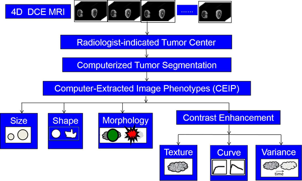
During the past several decades, efforts have been made by researchers in medical imaging to develop features that can be automatically extracted from images of lesions using analytical expressions. For this reason, these features are called human-engineered radiomic features (RAD_HE). Some of these, such as the largest dimension of the lesion, are geometric in basis [3]. Others describe texture using gray-level co-occurrence matrices, a method used to analyze images in many different applications in addition to medical imaging analysis [4]. When a contrast agent that changes the contrast of the tissue with respect to the biological basis of the imaging modality is injected into the subject, the dynamic response of the tissue to the uptake and washout of the agent can be measured quantitatively [5]. Features can also be extracted from apparent diffusion coefficient images [6], T2-weighted images [7], and diffusion MR images [8]. The investigation of features in the context of specific types of lesions, such as breast lesions that are less than 1 cm in diameter [9] or of specific molecular subtypes [10]–[13], can also be relevant. These features can collectively describe computer-extracted image phenotypes of a lesion. Fig. 1 shows an example workflow for extracting RAD_HE features from DCE-MR images of breast lesions.

Fig. 1.

Workflow for extracting human-engineered radiomic features (RAD_HE) from 4-D DCE-MR images for use in CADx.

The development of these human-engineered features based upon analytical expressions has contributed to the rise of the field of computer-aided diagnosis (CADx). CADx is a field of investigation in which extracted features are investigated for their relationship to a medical diagnosis, prognosis, or prediction question [14], [15]. At a basic level, regression analysis methods may be used, but machine learning methods, typically supervised in nature, have shown the strongest promise for investigating how such features may be used to predict disease or response to therapy. Classifiers, such as linear discriminant analysis or support vector machines (SVM), have been used to predict the class of lesions. Consequently, receiver operating characteristic curve (ROC) analysis is used to compare the predicted class of the lesions to the actual class (i.e., ground truth) and determine the true-positive fraction and the false-positive fraction across a range of thresholds [16]. The area under the ROC curve (AUC) is frequently used as a metric of performance, where AUC = 1 represents a classifier with perfect classification, and AUC = 0.5 represents classification no better than random guessing.

Artificial neural networks are computing systems designed to identify and merge features useful for distinguishing between classes of information using computing structures modeled after how neurons pass information among themselves. Convolutional neural networks (CNNs) are a subset of artificial neural networks. A given CNN is made up of an input and an output layer, with different possibilities of layers in between, called in total the architecture. These layers may be convolutional, pooling, or fully connected. While CNNs were initially introduced to medical image analysis in the 1980s [17], their rapid use was limited by computational power. Subsequent gains in computational power and the broader availability of graphical processing units have contributed to the use of CNNs for medical image analysis in the 21st century [18], [19].

The development of a CNN for image-based classification requires a very high number of images (on the order of millions) to learn what features may be useful for various classification questions. AlexNet [20] and VGG19 [21] are two networks that have been trained to identify several different classes within images, such as those of dogs or cats, which are called natural images. The development of custom CNNs trained from scratch for medical image classification tasks is a focus of ongoing investigation, but the needed collection of a large number of images in medical imaging classification questions is difficult to acquire. However, properties of a CNN pretrained for natural image classification can be used for other classification tasks, such as the classification of lesions as benign or malignant. This practice is called transfer learning, allowing neural network settings that were learned for one task to be transferred to another classification task.

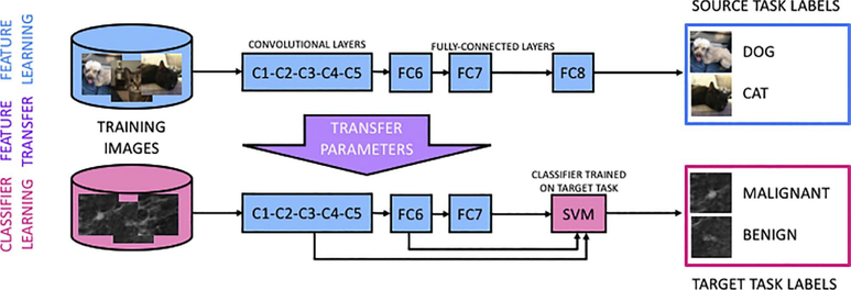
Two different types of transfer learning have been applied to medical imaging classification tasks. In fine-tuning, transfer learning involves the fine-tuning of weights that were developed from the initial training of the network using a large number of natural images for nonmedical classification tasks (CNN_FT). The network is intercepted at the latter layers and training is revised in the context of the medical images and the specific classification task. In feature extraction, after input of a medical image to a CNN, which had been previously trained on the nonmedical images, the outputs from different layers of the CNN serve as features to conventional classifiers (CNN_FE) (Fig. 2).

Fig. 2.

Transfer learning framework constructed for feature extraction for medical image classification (from [22]).

Each of these transfer learning methods involves several variables that must be investigated for the optimization of classification performance. For example, the outputs from several layers are available for feature extraction when CNNs are used, and the selection of them can be optimized [23]. The use of a CNN in CADx, whether trained from scratch or from transfer learning, can be referred to as CNN-based CADx.

Radiomics-based CADx (RAD_HE) and CNN-based CADx (CNN_FT or CNN_FE) both contribute to classification tasks in which they can yield a probability that a lesion, or some other general region of interest (ROI) in a medical image, is part of a certain class. However, between these CADx methods, there are differences that can influence their utility to a given classification question. For example, in radiomics-based CADx, the lesion is required to be segmented from its surrounding environment, and the extracted features represent the lesion itself. This, of course, places substantial dependence of later steps of the radiomics pipeline onto the segmentation method. Conversely, in CNN-based CADx, the features are extracted from images of an ROI that includes the lesion. Lesion segmentation or feature extraction using analytical expressions is not required. However, the selection of ROI around the lesion is relevant: inherently, some degree of background must be included, and it has been shown that the classification performance can depend upon the size of the ROI with respect to the tumor. If the ROI includes too much information, it hinders the classification of the lesion as there are essentially competing classification tasks.

The application of both radiomics- and CNN-based CADx to classification tasks in medical imaging, particularly in breast imaging [23]–[27], has shown promise. An additional area of investigation seeks to determine if these methods can be merged to improve classification performance, i.e., fusion CADx.

II. EXAMPLES OF TRANSFER LEARNING AND FUSION CLASSIFICATION IN CADx AND PROGNOSIS

While this is not a review article, an overview of our lab’s progress in transfer learning and fusion classification is described in the following to provide insight into the methodology presented in our newly reported study. While the new study uses MR images for the task of classification of lesions as malignant or benign, the methodology has been developed from our experience in using breast images from other modalities as well applied to classification tasks for cancer diagnosis and risk assessment. The various studies demonstrate, within this range of modalities and classification tasks, comparisons of performance using transfer learning and fusion methods to that achieved using human-engineered radiomic features.

A. Transfer Learning Using CNN-Feature Extraction (CNN_FE) From Full-Field Digital Mammography of the Breast

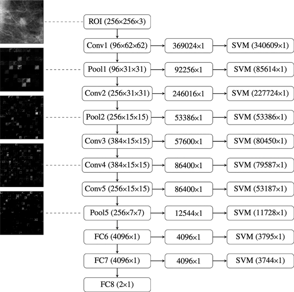
Transfer learning using CNN-based features was demonstrated in 2016 for the classification of 219 full-field digital mammography (FFDM) images of breast lesions as benign or cancer and compared to the classification performance using radiomics-based features from segmented lesions [23]. CNN-based features were extracted using AlexNet [20], a CNN model that has been pretrained on the ImageNet data set [28], comprised of over one million images and describing one thousand classes. The use of a CNN provided several layers from which features could be extracted (Fig. 3).

Fig. 3.

Illustration of the collection of layers at which features can be extracted from the pretrained AlexNet CNN during transfer learning. Right-most column: number of features for a given image that is used as input to a classifier (in this case, SVM). For each layer, these features were extracted from outputs from each layer, which were combined and flattened (center column) from their original image outputs (left column) (from [23]).

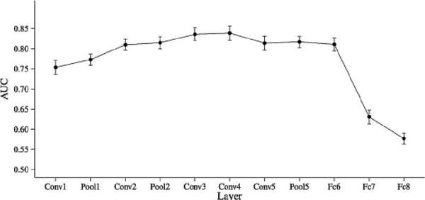
The study investigated the classification performance of features extracted at the different fully connected, convolutional, and max-pooling layers and selected an optimal layer (in this case, fully connected layer 6) due to its high predictive performance and relatively low dimensionality (Fig. 4).

Fig. 4.

Classification performance in the task of classification of mammographic lesions as benign or cancer, for classifiers based on features from each layer of AlexNet. Fully connected layer 6 (“Fc6” in the figure) was selected as the optimal layer for feature extraction, due to its high AUC performance and reduced computational cost (from Huynh et al. [23]).

Next, the radiomics-based and CNN-based methods were merged through a fusion classifier, constructed using soft voting to combine the outputs from the individual classifiers. While classification performance as measured by AUC was similar for the radiomics-based features (0.81 ± 0.03) and CNN-based features (0.81 ± 0.04) used separately for classification of lesions as benign or malignant, the fusion classifier produced statistically significant improvement in performance (0.86 ± 0.01), indicating that both RAD_HE and CNN_FE each provide unique information for the classification of the images.

B. Transfer Learning Using CNN-Feature Extraction (CNN_FE) and Fusion Classification Using Full-Field Digital Mammography, US, and MR Imaging of the Breast

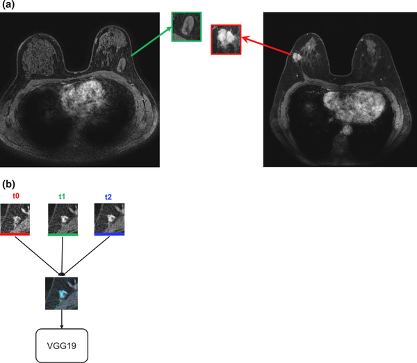
Transfer learning methods have been extended to other modalities [US and MR imaging (MRI)] and other pretrained CNNs (VGG19) for evaluation of classification performance in the task of distinguishing between breast lesions as benign or malignant [27]. The study investigated various methods within the transfer learning analysis pipeline, including preprocessing of ROIs and using features extracted from fully connected layers compared to those from max-pool layers. Another variation of image input was developed by using images from temporal 3-D image acquisition methods (DCE-MRI) into the three color channels of red-green-blue (RGB) images (Fig. 5).

Fig. 5.

Construction of an RGB image from ROIs extracted from multiple time points of a DCE-MR image series. (a) Full MR images of (left) benign lesion and (right) cancerous lesion. (b) ROIs from the precontrast time point (t0), first postcontrast time point (t1), and second postcontrast time point (t2) combined as one RGB image and input into the VGG19 CNN for feature extraction (from [27]).

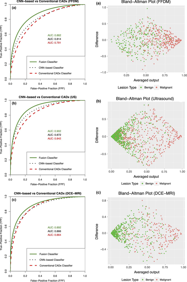
The study found moderate improvement in performance using pooled features extracted from the original size ROIs compared to using the fully connected features extracted from preprocessed ROIs. In addition, for each of the three modalities, the use of a fusion radiomics-based and CNN-based classifier in the task of classification of lesions as malignant or benign yielded performance better than either classifier on its own (Figs. 6 and 7), indicating that the use of fusion classifiers is valuable across multiple modalities.

Fig. 6.

Left column: comparison of classification performance for use of all three classifiers. Right column: associated Bland–Altman plot (from Antropova et al. [27]). (a) FFDM. (b) US. (c) DCE-MRI.

Fig. 7.

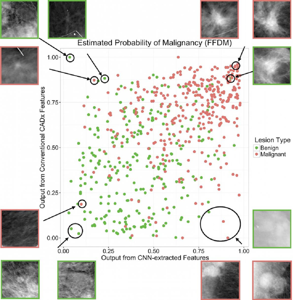
Classifier agreement plot for output from conventional features compared to output from CNN-extracted features (from Antropova et al. [27]).

C. Transfer Learning Using CNN-Feature Extraction (CNN_FE) From Digital Breast Tomosynthesis

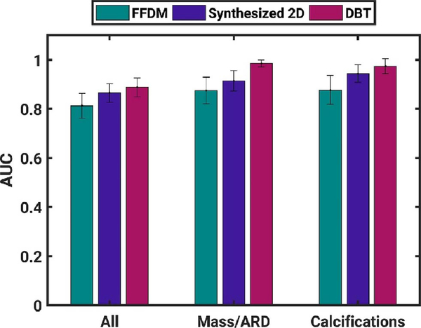
Transfer learning has also been applied to classification using FFDM and digital breast tomosynthesis (DBT), including associated synthesized 2-D images and key slices [22]. Within the consideration of modality and prepared images, classification performance was assessed for subsets of lesions that were mass/architectural distortion (ARD) or calcifications. Using VGG19, CNN features were extracted from craniocaudal (CC) and medial–lateral oblique (MLO) images and used as inputs to corresponding separate classifiers and, in addition, the outputs of the two classifiers were fused using soft voting to create a merged-view output. Classification performance was superior in both views for synthesized 2-D, for merged views for DBT, and for DBT when lesions were analyzed separately by mass/ARD and calcifications (Fig. 8).

Fig. 8.

Classification performance (AUC) in the task of classification of lesions as benign or malignant using a classifier merged from two different mammography views (CC and MLO). Error bars represent standard error (from [22]).

D. Transfer Learning Using CNN-Feature Extraction (CNN_FE) From Maximum Intensity Projection DCE-MR Images of the Breast

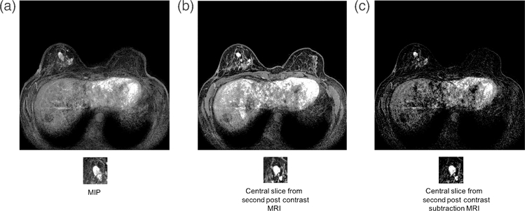
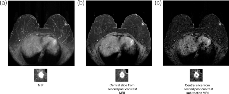
Further work in feature extraction using transfer learning investigated the use of images that incorporate spatial information. Maximum intensity projections (MIP) images were used for feature extraction using ConvNet VGGNet [29]. An MIP image is made by analyzing the gray-level values of each voxel in a stack of postcontrast subtraction images and assigning to that voxel in the MIP the maximum voxel value from the stack. The classification performance of CNN feature extraction from MIP images generated from the second postcontrast images was compared to that obtained using second postcontrast central slice and the second postcontrast subtraction central slice (Figs. 9 and 10).

Fig. 9.

Benign lesion image for (a) MIP image of the second postcontrast subtraction MRI, (b) center slice of the second postcontrast MRI, and (c) central slice of the second postcontrast subtraction MRI (from [29]).

Fig. 10.

Cancer image for (a) MIP image of the second postcontrast subtraction MRI, (b) center slice of the second postcontrast MRI, and (c) central slice of the second postcontrast subtraction MRI (from [29]).

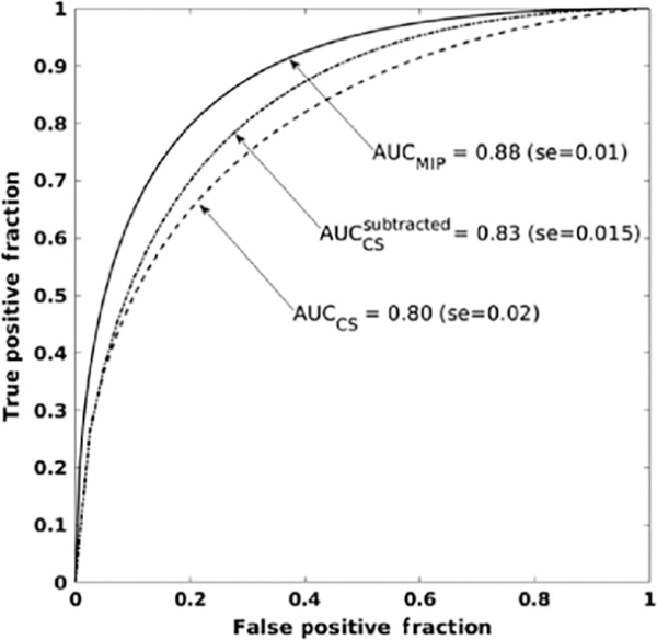
The MIP CNN demonstrated superior classification performance compared to using the second postcontrast images in either nonsubtraction or subtraction form (Fig. 11).

Fig. 11.

ROCs and associated AUC for the classification of lesions as benign or malignant using maximum intensity images (AUC_MIP), using center slice from second postcontrast images (AUC_CS) and subtracted second postcontrast images $\left(AU{C}_{CS}^{subtracted}\right)$ (from [29]).

E. Transfer Learning Using CNN Fine-Tuning (CNN_FT) and Long Short-Term Memory Networks on Breast DCE-MR Images

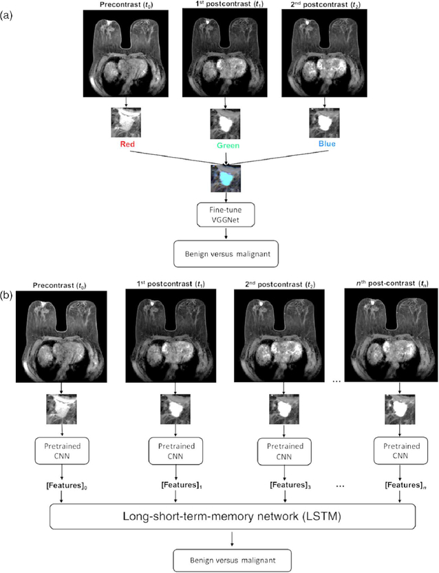
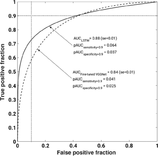
Temporal information from DCE-MRIs can be incorporated into deep learning methods using pretrained CNNs and long short-term memory (LSTM) networks. In a recent study, the VGG19 network was fine-tuned for the task of distinguishing between benign and malignant images by constructing RGB images from the precontrast and two postcontrast images via the three channels [30]. This architecture was compared to that when, instead of the RGB arrangement, various time-point MRIs were directly input to a CNN_FE with the subsequent outputs going to an LSTM architecture (Fig. 12). Classification performance was measured using AUC. Classification performance in the task of distinguishing between benign and malignant lesions was superior when using the LSTM, compared to using the fine-tuned VGG network (Fig. 13).

Fig. 12.

Radiomics pipeline for (a) images constructed from precontrast and first two postcontrast images, for which the VGG19 network was fine-tuned for the task of classification of images as benign or malignant. (b) Extraction of features using this pretrained CNN within LSTM network (from [30]).

Fig. 13.

ROC for the classification of lesions as benign or malignant using features extracted using a fine-tuned VGGnet or using LSTM (from [30]).

F. Transfer Learning Using CNN-Feature Extraction (CNN_FE) From Full-Field Digital Mammography of the Breast for Cancer Risk Assessment

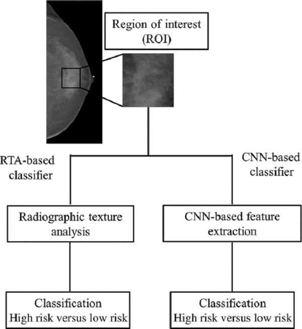
The studies described above involve the use of transfer learning for the task of diagnosing lesions as benign or malignant using images acquired from a variety of modalities. Risk assessment is an additional task for which transfer learning can be used. The analysis model for using transfer learning for risk assessment builds upon previous work, in which conventional radiographic texture analysis (RTA) was used to classify images of the breast according to risk. In that prior study, it was found that women at high risk tended to have dense breasts with parenchymal patterns that were coarse and of low contrast [31]. In a subsequent study [32], there two high-risk groups were involved: one of women with the BRCA1/2 gene mutation (36 with BRCA1 gene mutation and 17 with BRCA2 gene mutation) and one of 75 women with unilateral breast cancer. The low-risk group was comprised of 328 women undergoing screening mammography and who were considered to be at usual risk for developing breast cancer. For each case, features were extracted using either human-engineered RTA or a pretrained CNN for input to an SVM classifier (Fig. 14). ROC analysis was performed on the output from the classifiers as well as a fusion classifier created from the average of the classifier outputs.

Fig. 14.

Schematic of methods for the classification of ROIs using RTA (a conventional radiomics method) and CNN-based feature extraction (from [32]).

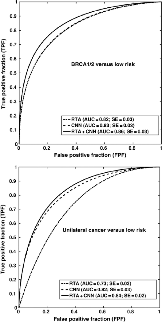
Two risk assessment tasks were investigated, where performance in the classification of ROIs as predictive of each of the high-risk groups as compared to the low-risk group was conducted for RTA, CNN_FE, and the fusion method. In the task of classification of ROIs as being from BRCA1/2 subjects versus low-risk subjects, classification performance using RTA or CNN_FE was comparable, while the fusion classifier resulted in a statistically significant improvement in performance. However, CNN_FE performed statistically significantly better than RTA in the task of distinguishing between ROIs from the contralateral breast in breast cancer cases versus those from the low-risk group (Fig. 15). It may be that the parenchymal patterns of women with the BRCA1/2 gene mutation have unique architecture compared to low-risk populations for which both RTA and CNN_FE yielded helpful distinguishing information.

Fig. 15.

Classification performance in the task of distinguishing between ROIs extracted from subjects with BRCA1/2 gene mutation or from a low-risk population (top) and distinguishing between ROIs extracted from subjects diagnosed with cancer in the contralateral breast or from a low-risk population (bottom) (from [32]).

III. COMPARISON OF HUMAN-ENGINEERED RADIOMICS VERSUS FINE - TUNING VERSUS FEATURE EXTRACTION

Our previously described studies involved focused investigations into the use of transfer learning in either its fine-tuning and feature-extraction forms compared to and fused with human-engineered radiomics. Another recent study, that by Truhn et al. [33], compared performance in the task of classification of breast lesions as malignant or benign using T2-weighted and DCE-MR images, separately for human-engineered radiomic features (extracted after manual segmentation of the lesions) and with a pretrained neural network. However, it would be useful to comprehensively investigate the different possibilities for the use of transfer learning, as well as the fusion of the classifiers that result from using them, compared to classification performance using human-engineered radiomics. Our study described below offers insight into understanding the methods and possibilities for the contributions of human-engineered radiomics, transfer learning, and fusion methods to CADx of breast cancer.

The breast DCE-MRI data set included in this article was retrospectively collected under a Health Insurance Portability and Accountability Act of 1996 (HIPAA)-compliant, Institutional Review Board-approved protocol with the waiver of consent. These MR imaging examinations were performed between 2015 and 2017 and included 1494 malignant lesions and 496 benign lesions based on the histopathology. There were 1494 malignant lesions from 1483 cancer patients, including eight bilateral and three bifocal cancer patients and 496 benign lesions from 496 benign patients. The clinical characteristics of the study population are listed in Tables 1 and 2. MR images were acquired with 3T GE scanners using a dedicated eight-channel phased-array breast coil with T1-weighted spoiled gradient sequence and gadolinium-diethylenetriamine pentaacetic acid (Gd-DTPA) as a contrast agent. Because our study made use of images commonly used by radiologists in their clinical interpretations, the images were not corrected for magnetic field inhomogeneity, and intrapatient standardization of image intensities was not conducted. However, it is important to note that the evaluation was conducted on an independent testing set, as described in the following.

Table 1.

Clinical Characteristics of the Study Population

		Training Data		Testing Data
		Malignant	Benign	Malignant	Benign
	Age (years) mean [range]	47.6 [19–77]	42.2 [16–76]	49.3 [25–75]	41.9 [19–65]
	Size (mm) mean ± standard deviation	19.1 ± 8.6	14.7 ± 10.7	18.5 ± 7.6	12.9 ± 6.8
Lesion type	Mass (percent of dataset)	716 (75.7%)	230 (24.3%)	293 (80.7%)	70 (19.3%)
	Non-mass enhancement (NME) (percent of dataset)	357 (70.1%)	152 (29.9%)	128 (74.4%)	44 (25.6%)

Table 2.

Radiologists’ BI-RADS Categorization of the Study Population (Number of Lesions in Each Category)

MRI BI-RADS Categorization	0	1	2	3	4	5	6
Malignant	0	0	0	4	472	752	266
Benign	2	3	4	252	230	5	0

The radiologists’ classification performance in the task of distinguishing between lesions as malignant or benign may be approximated using their clinically reported BI-RADS scores as the decision variable for input to ROC analysis to calculate AUC. For this data set, evaluated by patients, AUC = 0.92 when utilizing the radiologists’ BI-RADS scores. However, it is important to note that an AUC calculated from BI-RADS data should be cautiously used to estimate radiologists’ performance due to the necessity in ROC analysis that the input decision variable be on an ordinal scale, which BI-RADS is not [34].

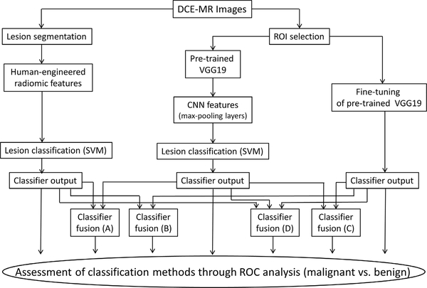
In order to minimize the bias in case selection for the computerized image analysis, the data set was divided into a training data set and an independent testing data set. The training data set included cases from the years 2015 and 2016, and the testing data set included cases from year 2017. There was one lesion per patient in the testing data set. Three different primary types of classification were performed in this article: human-engineered radiomics (Rad_HE), CNN-based feature extraction (CNN_FE), and CNN-based fine-tuning (CNN_FT). In addition, four different types of fusion classifiers were used. All are described in the following. Fig. 16 shows a schematic of the seven various classification methods.

Fig. 16.

Schematic of various classification methods in the task of differentiating malignant from benign breast lesions on DCE-MRI, including the classification with human-engineered radiomic features (Rad_HE), with CNN-based feature extraction (CNN_FE), with CNN-based fine tuning (CNN_FT), and four fusion classifiers.

A. Human-Engineered Radiomics (Rad_HE)

Human-engineered radiomic features (Rad_HE) were collected using the following methods. The lesion location on each MR image was indicated by an expert radiologist. Each lesion was then automatically segmented from the DCE-MR images for each lesion, in 3-D, from the surrounding parenchyma using a fuzzy c-means clustering method [35] using the radiologist-indicated lesion location. Thirty-eight human-engineered 3-D radiomic features were automatically extracted from the 3-D lesion volume for each lesion to characterize lesion size, shape, morphology, enhancement texture, kinetics, and enhancement-variance kinetics [3], [5], [36], [37] (Table 3). All time-point images were used to calculate the kinetic-related radiomic features. The 3-D texture features of each computer-extracted lesion volume were calculated on the first post contrast images, using a 32-binned co-occurrence matrix [36]. An SVM classifier was trained on the cases from the years 2015 and 2016 (training data set), while the year 2017 cases served as the independent testing data set in the task of distinguishing between malignant and benign lesions. Output from the SVM served as the decision variable for input to ROC analysis.

Table 3.

Human-Engineered Radiomic Features (RAD_HE) and Their Descriptions

Image Feature	Feature Description	Reference
Volume (mm3) (S1)	Volume of lesion	[3]
Effective diameter (mm) (S2)	Greatest dimension of a sphere with the same volume as the lesion
Surface area (mm2) (S3)	Lesion surface area
Maximum linear size (mm) (S4)	Maximum distance between any 2 voxels in the lesion
Sphericity (G1)	Similarity of the lesion shape to a sphere
Irregularity (G2)	Deviation of the lesion surface from the surface of a sphere
Surface area/volume (1/mm) (G3)	Ratio of surface area to volume
Margin sharpness (M1)	Mean of the image gradient at the lesion margin
Variance of margin sharpness (M2)	Variance of the image gradient at the lesion margin
Variance of radial gradient histogram (M3)	Degree to which the enhancement structure extends in a radial pattern originating from the center of the lesion
Contrast (T1)	Location image variations	[36]
Correlation (T2)	Image linearity
Difference entropy (T3)	Randomness of the difference of neighboring voxels’ gray-levels
Difference variance (T4)	Variations of difference of gray-levels between voxel-pairs
Energy (T5)	Image homogeneity
Entropy (T6)	Randomness of the gray-levels
Inverse difference moment (homogeneity) (T7)	Image homogeneity
Information measure of correlation 1 (T8)	Nonlinear gray-level dependence
Information measure of correlation 2 (T9)	Nonlinear gray-level dependence
Maximum correlation coefficient (T10)	Nonlinear gray-level dependence
Sum average (T11)	Overall brightness
Sum entropy (T12)	Randomness of the sum of gray-levels of neighboring voxels
Sum variance (T13)	Spread in the sum of the gray-levels of voxel-pairs distribution
Sum of squares (variance) (T14)	Spread in the gray-level distribution
Maximum enhancement (K1)	Maximum contrast enhancement	[5]
Time to peak (s) (K2)	Time at which the maximum enhancement occurs
Uptake rate (1/s) (K3)	Uptake speed of the contrast enhancement
Washout rate (1/s) (K4)	Washout speed of the contrast enhancement
Curve shape index (K5)	Difference between late and early enhancement
Enhancement at first postcontrast time point (K6)	Enhancement at first post-contrast time point
Signal enhancement ratio (K7)	Ratio of initial enhancement to overall enhancement
Volume of most enhancing voxels (mm3) (K8)	Volume of the most enhancing voxels
Total rate variation (1/s2) (K9)	How rapidly the contrast will enter and exit from the lesion
Normalized total rate variation (1/s2) (K10)	How rapidly the contrast will enter and exit from the lesion
Maximum enhancement-variance (E1)	Maximum spatial variance of contrast enhancement over time	[37]
Enhancement-variance time to peak (s) (E2)	Time at which the maximum variance occurs
Enhancement variance-increasing rate (1/s) (E3)	Rate of increase of the enhancement-variance during uptake
Enhancement-variance decreasing rate (1/s) (E4)	Rate of decrease of the enhancement-variance during washout

B. CNN Feature Extraction (CNN_FE)

For CNN feature extraction, the VGG19 model [21] pretrained on the ImageNet [28] data set was used. The VGG19 model consists of 19 weight layers, including five stacks of convolutional layers with each stack containing two or four convolutional layers and a max-pooling layer, and followed by three fully connected layers. For each lesion, the central slice (i.e., the slice containing the most lesion voxels) was identified. Since VGG19 takes an RGB image as an input, an ROI containing the breast lesion extracted from the precontrast, first postcontrast, and second postcontrast central slice DCE-MR images was input to the three channels to form an RGB image. Variable sizes of RGB ROIs were resized to 224 × 224 × 3 pixels to conform to the training images used in the pretrained VGG19. CNN features were extracted from five max-pooling layers and then average-pooled on each max-pooling layer to reduce the number of features. These CNN features were then normalized to form a final CNN feature vector for the subsequent SVM classifier. The analysis was conducted similarly as we did for the human-engineered radiomic method, i.e., using years 2015 and 2016 cases for the training and year 2017 cases for the independent testing in the task of distinguishing malignant from benign lesions. Output from the SVM served as the decision variable for input to ROC analysis.

C. CNN Fine-Tuning (CNN_FT)

For CNN fine-tuning, the pretrained VGG19 was used, with the weights of early layers being frozen. We replaced the final fully connected layer with a fully connected layer of 100 classes, a fully connected layer of two classes, and a softmax layer, which underwent training. The output from the softmax layer served as the decision variable for the input to ROC analysis. The initial learning rate for network training was set at 0.0002 with a drop factor of 0.1 and drop periods of 5 epochs using stochastic gradient descent as an optimizer. The training data set, MRI cases from years 2015 and 2016, was split into 80% for training and 20% for validation, and the year 2017 cases were used for independent testing in the task of distinguishing malignant from benign lesions.

D. Fusion Classifiers

In addition to human-engineered radiomics and CNN-based classifiers, fusion classifiers were also evaluated. The fusion classifier was constructed by averaging the outputs from each of the individual classifiers, with the output of each fusion serving as the decision variable for input to ROC analysis. Four fusion classifiers were constructed in the study as follows.

1. FusionA: Fusion of human-engineered radiomics (Rad_HE) and CNN feature extraction (CNN_FE).

2. FusionB: Fusion of human-engineered radiomics (Rad_HE) and CNN fine-tuning (CNN_FT).

3. FusionC: Fusion of CNN feature extraction (CNN_FE) and CNN fine-tuning (CNN_FT).

4. FusionD: Fusion of human-engineered radiomics (Rad_HE), CNN feature extraction (CNN_FE), and CNN fine-tuning (CNN_FT).

E. Statistical Comparisons

All the classification methods were evaluated on all lesions in the independent test set including both mass and nonmass enhancement (NME), mass lesions only, and NME lesions only. The performances of the classifiers were evaluated using ROC analysis [38], yielding AUC (and standard error), which was used as a figure of merit to assess the performance of each classifier in the task of distinguishing malignant from benign lesions. The statistical significance for the difference between the performances of classifiers was evaluated using ROCKIT software [39]. The Bonferroni–Holm method [40] was applied to correct for multiple comparisons. Sensitivity and specificity for the classification output of each classifier method were determined by selecting a cutoff value that minimizes m = (1 − sensitivity)²+ (1 − specificity)² [33] (Table 4).

Table 4.

Sensitivity and Specificity of the Data Set for Each Classifier, Using a Metric for Cut-Off Value That Minimizes m = (1 − Sensitivity)² + (1 − Specificity)². Because all Lesions Were Referred for Biopsy, the Sensitivity and Specificity of the Data Set Were Not Calculated For Clinical Assessment

Classifier	RadHE	CNNFE	CNNFT	FusionA	FusionB	FusionC	FusionD
Sensitivity (%) (fraction of cases)	83.6 (352/421)	79.8 (336/421)	81.5 (343/421)	84.8 (357/421)	80.0 (337/421)	84.3 (355/421)	86.2 (363/421)
Specificity (%) (fraction of cases)	83.3 (95/114)	78.9 (90/114)	85.1 (97/114)	84.2 (96/114)	87.7 (100/114)	81.6 (93/114)	81.6 (93/114)

F. Results

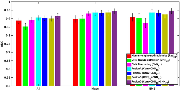
For the human-engineered radiomic method, AUC values of 0.89, 0.90, and 0.91 were obtained in the task of distinguishing between malignant and benign lesions across all lesions, mass lesions only, and NME lesions only, respectively (Fig. 17 and Table 5, which includes p-values and confidence intervals of the comparisons). For the CNN feature extraction method (CNN_FE), AUC values of 0.85, 0.90, and 0.90 were obtained in the classification tasks across all lesions, mass lesions only, and NME lesions, respectively. For the CNN fine-tuning method (CNN_FT), AUC values of 0.89, 0.93, and 0.87 were obtained in the classification tasks across all lesions, mass lesions only, and NME lesions only, respectively.

Fig. 17.

AUC values from various classifiers, including human-engineered radiomics (Rad_HE), CNN-based feature extraction (CNN_FE), CNN-based fine tuning (CNN_FT), FusionA (Rad_HE + CNN_FE), FusionB (Rad_HE + CNN_FT), FusionC (CNN_FE + CNN_FT), and FusionD (Rad_HE + CNN_FE + CNN_FT) on entire data set including both mass and NME lesions, mass lesions only, and NME lesions only. Error bars show one standard error.

Table 5.

Classification Performance in the Task of Distinguishing Malignant From Benign Breast Lesions for the Human-Engineered Radiomics, CNN Feature Extraction, CNN Fine-Tuning, and Fusion Classifiers on Entire Data Set (Both Mass and NME), Mass Lesion Only, and NME Only. The Multiple Comparison Corrections Were Performed Using the Bonferroni–Holm Method

	All		Mass		NME
	AUC [95% CI]	p-value for ΔAUC (significance level) [95% CI of ΔAUC]	AUC [95% CI]	p-value for ΔAUC (significance level) [95% CI of ΔAUC]	AUC [95% CI]	p-value for ΔAUC (significance level) [95% CI of ΔAUC]
Human-engineered radiomics (RadHE)	0.89 [0.8582, 0.9221]	...	0.90 [0.8546, 0.9348]	...	0.91 [0.8579, 0.9488]	...
CNN feature extraction (CNNFE)	0.85 [0.8158, 0.8903]	...	0.90 [0.8520, 0.9307]	...	0.90 [0.8423, 0.9466]	...
FusionA (RadHE + CNNFE)	0.91 [0.8732, 0.9352]	...	0.94 [0.9032, 0.9648]	...	0.94 [0.8808, 0.9650]	...
RadHE vs CNNFE	...	0.0619 (0.025) [−0.0019, 0.0780]	...	0.8722 (0.05) [−0.0426, 0.0502)	...	0.7933 (0.05) [−0.0468, 0.0613]
RadHE vs FusionA	...	0.2499 (0.05) [−0.0297, 0.0077]	...	0.0057 (0.025) [−0.0637, −0.0109]	...	0.1703 (0.025) [−0.0452, 0.0080]
CNNFE vs FusionA	...	0.0002 (0.017) [−0.0735, −0.0228]	...	0.0039 (0.017) [−0.0650, −0.0124]	...	0.1663 (0.017) [−0.0596, 0.0103]
Human-engineered radiomics (RadHE)	0.89 [0.8582, 0.9221]	...	0.90 [0.8546, 0.9348]	...	0.91 [0.8579, 0.9488]	...
CNN fine-tuning (CNNFT)	0.89 [0.8582, 0.9245]	...	0.93 [0.8971, 0.9547]	...	0.87 [0.8075, 0.9169]	...
FusionB (RadHE + CNNFT)	0.90 [0.8659, 0.9334]	...	0.93 [0.8961, 0.9625]	...	0.93 [0.8776, 0.9604]	...
RadHE vs CNNFT	...	0.9955 (0.05) [−0.0281, 0.0279]	...	0.1001 (0.025) [−0.0630, 0.0055]	...	0.1469 (0.05) [−0.0145, 0.0968]
RadHE vs FusionB	...	0.1490 (0.017) [−0.0244, 0.0037]	...	0.0002 (0.017) [−0.0500, −0.0153]	...	0.1259 (0.025) [−0.0437, 0.0054]
CNNFT vs FusionB	...	0.1671 (0.025) [−0.0289, 0.0050]	...	0.7357 (0.05) [−0.0235, 0.0166]	...	0.0037 (0.017) [−0.1018, −0.0197]
CNN feature extraction (CNNFE)	0.85 [0.8158, 0.8903]	...	0.90 [0.8520, 0.9307]	...	0.90 [0.8423, 0.9466]	...
CNN fine-tuning (CNNFT)	0.89 [0.8582, 0.9245)	...	0.93 [0.8971, 0.9547]	...	0.87 [0.8075, 0.9169]	...
FusionC (CNNFE + CNNFT)	0.90 [0.8737, 0.9319]		0.94 [0.9020, 0.9584]	...	0.92 [0.8769, 0.9583]	...
CNNFE vs CNNFT	...	0.0481 (0.025) [−0.0761, −0.0003]	...	0.0886 (0.025) [−.0708, 0.0050]	...	0.2441 (0.025) [−0.0237, 0.0933]
CNNFE vs FusionC	...	<0.0001 (0.017) [−0.0651, −0.0255]	...	0.0006 (0.017) [−0.0534, −0.0145]	...	0.2448 (0.05) [−0.0463, 0.0118]
CNNFT vs FusionC	...	0.4302 (0.05) [−0.0286, 0.0122]	...	0.7327 (0.05) [−0.0251, 0.0177]	...	0.0034 (0.017) [−0.0887, −0.0176]
Human-engineered radiomics (RadHE)	0.89 [0.8582, 0.9221]	...	0.90 [0.8546, 0.9348]	...	0.91 [0.8579, 0.9488]	...
CNN feature extraction (CNNFE)	0.85 [0.8158, 0.8903]	...	0.90 [0.8520, 0.9307]	...	0.90 [0.8423, 0.9466]	...
CNN fine-tuning (CNNFT)	0.89 [0.8582, 0.9245)	...	0.93 [0.8971, 0.9547]	...	0.87 [0.8075, 0.9169]	...
FusionD (RadHE + CNNFE+CNNFT)	0.91 [0.8840, 0.9431]	...	0.94 [0.9122, 0.9678]	...	0.95 [0.9066, 0.9735]	...
RadHE vs FusionD	...	0.0448 (0.025) [−0.0381, −0.0004]	...	0.0018 (0.025) [−0.0697, −0.0160]	...	0.0171 (0.025) [−0.0643, −0.0063]
CNNFE vs FusionD	...	0.0001 (0.017) [−0.0842, −0.0285]	...	0.0015 (0.017) [−0.0737, −0.0175)	...	0.0337 (0.05) [−0.0829, −0.0033]
CNNFT vs FusionD	...	0.0509 (0.05) [−0.0393, 0.0001]	...	0.1724 (0.05) [−0.0345, 0.0062]	...	0.0004 (0.017) [−0.1186, −0.0344]

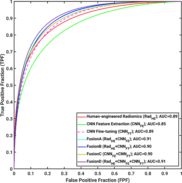
ROC curves for all seven classifiers are shown in Fig. 18 for the group of all lesions.

Fig. 18.

ROC analysis results on the entire data set, including both mass and NME lesions with cases from the years 2015 and 2016 as training data set and cases from the year 2017 as testing data set in the tasking of distinguishing between malignant from benign lesions on DCE-MRI.

While the AUCs for these classifiers ranged from 0.85 to 0.91 and are thus slightly less than the AUC acquired using the radiologists’ BI-RADS alone (described above, AUC = 0.92), it is important to reiterate that the AUC from ROC analysis of BI-RADS data is not able to be compared to AUCs determined from ordinal scale data [34], which has been the focus of our study.

Inspection of Table 2 indicates that classification using BI-RADS data alone shows that BI-RADS is highly sensitive but not very specific. Table 4 demonstrates that across all classifiers used in this article, both the sensitivity and specificity are high.

For the two CNN-based methods alone, improved classification performances were observed from CNN feature extraction to CNN fine-tuning methods, from 0.85 to 0.89 for all lesions, and from 0.90 to 0.93 for mass lesions only. When only NME lesions were used in this scenario, AUC values slightly decreased from 0.90 to 0.87. This may be due to the small size of the training data set of NME lesions used in fine-tuning the VGG19 model.

For the four fusion methods assessed in the study, improved classification performances on the independent test set were observed for all four fusion classifiers compared with human-engineered radiomics, CNN feature extraction, or CNN fine-tuning on all lesions, mass lesions only, NME lesions only, respectively, although sometimes the data failed to show the statistical significance in terms of the difference of the performance of the classifiers.

IV. DISCUSSION AND CONCLUSION

The goal of our novel study here was to comprehensively summarize and build on our prior research and evaluate the performance of human-engineered radiomics and deep learning methods in the task of distinguishing between benign or malignant lesions. The classification methods used human-engineered radiomic features as well as two variations on transfer learning: features extracted from pretrained CNNs or features extracted after fine-tuning of a CNN. Four different associated fusion classifiers formed by combinations of the three sets of extracted features were also investigated. The work presented here is also novel in its investigation of these classification performance variations in the context of lesions in both non mass and mass enhancement forms. Advantages of this article include that all images were collected at the same field strength (3T), eliminating possible variation in feature values due to field strength. The selection of training and testing data sets in terms of year of acquisition also reduced bias in case selection.

From the literature, our results are mostly comparable and, in some cases, higher than the classification performances reported by Truhn et al. [33] in their investigation into using radiomic and CNN-based methods separately for the classification of breast lesions as malignant or benign with T2-weighted and DCE-MR images. In their study, CNN-based methods demonstrated AUC values of 0.83 and 0.88, while methods using radiomic features yielded AUC values from 0.78 to 0.81 for their data set on which the radiologists’ BI-RADS AUC was 0.98, indicating a slightly easier discrimination task for the radiologists.

Future work will examine CNN activation maps to understand the vast amount of relevant and irrelevant information that results from transfer learning, and their role and effect in dimension reduction, feature extraction, and feature merging. Such investigations will also assist in understanding the synergistic nature of fusion classification using CNN-based transfer learning and human-engineered radiomic features, as the results of this article highlight the improvement in classification performance from using fusion techniques, compared to using either human-engineered radiomic features or features extracted from CNN transfer learning alone.

ABOUT THE AUTHORS

Heather M. Whitney is an Associate Professor of physics with Wheaton College, Wheaton, IL, USA, and a Visiting Scholar with the Department of Radiology, The University of Chicago, Chicago, IL, USA. Her experience in quantitative medical imaging has ranged from polymer gel dosimetry to radiation damping in nuclear magnetic resonance to now focusing on computer-aided diagnosis (CADx) of breast cancer imaging. She is interested in investigating the effects of the physical basis of imaging on CADx, as well as the repeatability and robustness of CADx.

Hui Li is a Research Associate Professor of radiology with The University of Chicago, Chicago, IL, USA, and has been involved in quantitative imaging analysis on medical images for over a decade. His research interests include breast cancer risk assessment, diagnosis, prognosis, response to therapy, understanding the relationship between radiomics and genomics, and their future roles in precision medicine with both conventional and deep learning approaches.

Yu Ji was a Visiting Scholar with the Department of Radiology, The University of Chicago, Chicago, IL, USA. He is currently an Attending Physician with the Department of Breast Imaging, Tianjin Medical University Cancer Institute and Hospital, Tianjin, China. He has been working for over five years on mammography, ultrasound, and magnetic resonance imaging (MRI). His current research interests include quantitative image analysis in breast cancer diagnosis, prognosis, and response to therapy.

Peifang Liu is currently the Director of the Department of Breast Imaging, Tianjin Medical University Cancer Institute and Hospital, Tianjin, China. She has been working, for several decades, in mammography, ultrasound, and magnetic resonance imaging. Her research interests include breast cancer diagnosis and management.

Maryellen L. Giger (Fellow, IEEE) is the A. N. Professor of Radiology/Medical Physics with The University of Chicago, Chicago, IL, USA, and has been working, for multiple decades, in computer-aided diagnosis/computer vision/machine learning/deep learning in cancer diagnosis and management. Her research interests include understanding the role of quantitative radiomics and machine learning in personalized medicine.

REFERENCES

- [1].Siegel RL, Miller KD, and Jemal A, “Cancer statistics, 2019,” CA, Cancer J. Clinicians, vol. 69, no. 1, pp. 7–34, 2019. [DOI] [PubMed] [Google Scholar]
- [2].D’Orsi CJ et al. , ACR BI-RADS Atlas, Breast Imaging and Data System. Reston, VA, USA: American College of Radiology, 2013. [Google Scholar]
- [3].Gilhuijs KGA, Giger ML, and Bick U, “Computerized analysis of breast lesions in three dimensions using dynamic magnetic-resonance imaging,” Med. Phys, vol. 25, no. 9, pp. 1647–1654, 1998. [DOI] [PubMed] [Google Scholar]
- [4].Chitalia RD and Kontos D, “Role of texture analysis in breast MRI as a cancer biomarker: A review,” J. Magn. Reson. Imag, vol. 49, no. 4, pp. 927–938, Apr. 2019. [DOI] [PMC free article] [PubMed] [Google Scholar]
- [5].Chen W, Giger ML, Bick U, and Newstead GM, “Automatic identification and classification of characteristic kinetic curves of breast lesions on DCE-MRI,” Med. Phys, vol. 33, no. 8, pp. 2878–2887, 2006. [DOI] [PubMed] [Google Scholar]
- [6].Hu B, Xu K, Zhang Z, Chai R, Li S, and Zhang L, “A radiomic nomogram based on an apparent diffusion coefficient map for differential diagnosis of suspicious breast findings,” Chin. J. Cancer Res, vol. 30, no. 4, pp. 432–438, 2018. [DOI] [PMC free article] [PubMed] [Google Scholar]
- [7].Gallego-Ortiz C and Martel AL, “Using quantitative features extracted from T2-weighted MRI to improve breast MRI computer-aided diagnosis (CAD),” PLoS One, vol. 12, no. 11, Nov. 2017, Art. no. e0187501. [DOI] [PMC free article] [PubMed] [Google Scholar]
- [8].Bickelhaupt S et al. , “Prediction of malignancy by a radiomic signature from contrast agent-free diffusion MRI in suspicious breast lesions found on screening mammography,” J. Magn. Reson. Imag, vol. 46, no. 2, pp. 604–616, Aug. 2017. [DOI] [PubMed] [Google Scholar]
- [9].Gibbs P et al. , “Characterization of sub-1 cm breast lesions using radiomics analysis,” J. Magn. Reson. Imag, vol. 50, no. 5, pp. 1468–1477, Nov. 2019. [DOI] [PMC free article] [PubMed] [Google Scholar]
- [10].Mazurowski MA, Zhang J, Grimm LJ, Yoon SC, and Silber JI, “Radiogenomic analysis of breast cancer: Luminal b molecular subtype is associated with enhancement dynamics at MR imaging,” Radiology, vol. 273, no. 2, pp. 365–372, 2014. [DOI] [PubMed] [Google Scholar]
- [11].Wang J et al. , “Identifying triple-negative breast cancer using background parenchymal enhancement heterogeneity on dynamic contrast-enhanced MRI: A pilot radiomics study,” PLoS One, vol. 10, no. 11, 2015, Art. no. e0143308. [DOI] [PMC free article] [PubMed] [Google Scholar]
- [12].Wu J et al. , “Identifying relations between imaging phenotypes and molecular subtypes of breast cancer: Model discovery and external validation,” J. Magn. Reson. Imag, vol. 46, no. 4, pp. 1017–1027, 2017. [DOI] [PMC free article] [PubMed] [Google Scholar]
- [13].Whitney HM et al. , “Additive benefit of radiomics over size alone in the distinction between benign lesions and luminal a cancers on a large clinical breast MRI dataset,” Acad. Radiol, vol. 26, no. 2, pp. 202–209, 2019. [DOI] [PMC free article] [PubMed] [Google Scholar]
- [14].Giger ML, Karssemeijer N, and Schnabel JA, “Breast image analysis for risk assessment, detection, diagnosis, and treatment of cancer,” Annu. Rev. Biomed. Eng, vol. 15, pp. 327–357, Jul. 2013. [DOI] [PubMed] [Google Scholar]
- [15].Yip SSF and Aerts HJWL, “Applications and limitations of radiomics,” Phys. Med. Biol, vol. 61, no. 13, pp. R150–R166, 2016. [DOI] [PMC free article] [PubMed] [Google Scholar]
- [16].Metz CE, “Basic principles of ROC analysis,” Seminars Nucl. Med, vol. 8, no. 4, pp. 283–298, Oct. 1978. [DOI] [PubMed] [Google Scholar]
- [17].Zhang W, Doi K, Giger ML, Wu Y, Nishikawa RM, and Schmidt RA, “Computerized detection of clustered microcalcifications in digital mammograms using a shift-invariant artificial neural network,” Med. Phys, vol. 21, no. 4, pp. 517–524, 1994. [DOI] [PubMed] [Google Scholar]
- [18].Sahiner B et al. , “Deep learning in medical imaging and radiation therapy,” Med. Phys, vol. 46, no. 1, pp. e1–e36, Jan. 2019. [DOI] [PMC free article] [PubMed] [Google Scholar]
- [19].Bi WL et al. , “Artificial intelligence in cancer imaging: Clinical challenges and applications,” CA, Cancer J. Clinicians, vol. 69, no. 2, pp. 127–157, Mar-Apr 2019. [DOI] [PMC free article] [PubMed] [Google Scholar]
- [20].Krizhevsky A, Sutskever I, and Hinton GE, “ImageNet classification with deep convolutional neural networks,” in Proc. Adv. Neural Inf. Process. Syst, 2012, pp. 1097–1105. [Google Scholar]
- [21].Simonyan K and Zisserman A, “Very deep convolutional networks for large-scale image recognition,” 2014, arXiv:1409.1556. [Online]. Available: https://arxiv.org/abs/1409.1556 [Google Scholar]
- [22].Mendel K, Li H, Sheth D, and Giger M, “Transfer learning from convolutional neural networks for computer-aided diagnosis: A comparison of digital breast tomosynthesis and full-field digital mammography,” Acad. Radiol, vol. 26, no. 6, pp. 735–743, Jun. 2019. [DOI] [PMC free article] [PubMed] [Google Scholar]
- [23].Huynh BQ, Li H, and Giger ML, “Digital mammographic tumor classification using transfer learning from deep convolutional neural networks,” J. Med. Imag, vol. 3, no. 3, 2016, Art. no. 034501. [DOI] [PMC free article] [PubMed] [Google Scholar]
- [24].Aboutalib SS, Mohamed AA, Berg WA, Zuley ML, Sumkin JH, and Wu S, “Deep learning to distinguish recalled but benign mammography images in breast cancer screening,” Clin. Cancer Res, vol. 24, no. 23, pp. 5902–5909, Dec. 2018. [DOI] [PMC free article] [PubMed] [Google Scholar]
- [25].Gastounioti A, Oustimov A, Hsieh M-K, Pantalone L, Conant EF, and Kontos D, “Using convolutional neural networks for enhanced capture of breast parenchymal complexity patterns associated with breast cancer risk,” Acad. Radiol, vol. 25, no. 8, pp. 977–984, Aug. 2018. [DOI] [PMC free article] [PubMed] [Google Scholar]
- [26].Byra M et al. , “Breast mass classification in sonography with transfer learning using a deep convolutional neural network and color conversion,” Med. Phys, vol. 46, no. 2, pp. 746–755, Feb. 2019. [DOI] [PMC free article] [PubMed] [Google Scholar]
- [27].Antropova N, Huynh BQ, and Giger ML, “A deep feature fusion methodology for breast cancer diagnosis demonstrated on three imaging modality datasets,” Med. Phys, vol. 44, no. 10, pp. 5162–5171, 2017. [DOI] [PMC free article] [PubMed] [Google Scholar]
- [28].Deng J, Dong W, Socher R, Li L-J, Li K, and Fei-Fei L, “ImageNet: A large-scale hierarchical image database,” in Proc. IEEE Conf. Comput. Vis. Pattern Recognit., Jun. 2009, pp. 248–255. [Google Scholar]
- [29].Antropova NO, Abe H, and Giger ML, “Use of clinical MRI maximum intensity projections for improved breast lesion classification with deep convolutional neural networks,” J. Med. Imag, vol. 5, no. 1, 2018, Art. no. 014503. [DOI] [PMC free article] [PubMed] [Google Scholar]
- [30].Antropova N, Huynh B, Li H, and Giger ML, “Breast lesion classification based on dynamic contrast-enhanced magnetic resonance images sequences with long short-term memory networks,” J. Med. Imag, vol. 6, no. 1, 2018, Art. no. 011002. [DOI] [PMC free article] [PubMed] [Google Scholar]
- [31].Li H et al. , “Computerized analysis of mammographic parenchymal patterns on a large clinical dataset of full-field digital mammograms: Robustness study with two high-risk datasets,” J. Digit. Imag, vol. 25, no. 5, pp. 591–598, Oct. 2012. [DOI] [PMC free article] [PubMed] [Google Scholar]
- [32].Li H, Giger ML, Huynh BQ, and Antropova NO, “Deep learning in breast cancer risk assessment: Evaluation of convolutional neural networks on a clinical dataset of full-field digital mammograms,” J. Med. Imag, vol. 4, no. 4, 2017, Art. no. 041304. [DOI] [PMC free article] [PubMed] [Google Scholar]
- [33].Truhn D, Schrading S, Haarburger C, Schneider H, Merhof D, and Kuhl C, “Radiomic versus convolutional neural networks analysis for classification of contrast-enhancing lesions at multiparametric breast MRI,” Radiology, vol. 290, no. 3, pp. 290–297, 2019. [DOI] [PubMed] [Google Scholar]
- [34].Jiang Y and Metz CE, “BI-RADS data should not be used to estimate ROC curves,” Radiology, vol. 256, no. 1, pp. 29–31, 2010. [DOI] [PMC free article] [PubMed] [Google Scholar]
- [35].Chen W, Giger ML, and Bick U, “A fuzzy c-means (FCM)-based approach for computerized segmentation of breast lesions in dynamic contrast-enhanced MR images,” Acad. Radiol, vol. 13, no. 1, pp. 63–72, 2006. [DOI] [PubMed] [Google Scholar]
- [36].Chen W, Giger ML, Li H, Bick U, and Newstead GM, “Volumetric texture analysis of breast lesions on contrast-enhanced magnetic resonance images,” Magn. Reson. Med, vol. 58, no. 3, pp. 562–571, 2007. [DOI] [PubMed] [Google Scholar]
- [37].Chen W, Giger ML, Lan L, and Bick U, “Computerized interpretation of breast MRI: Investigation of enhancement-variance dynamics,” Med. Phys, vol. 31, no. 5, pp. 1076–1082, 2004. [DOI] [PubMed] [Google Scholar]
- [38].Metz CE, “Some practical issues of experimental design and data analysis in radiological ROC studies,” Invest. Radiol, vol. 24, no. 3, pp. 234–245, 1989. [DOI] [PubMed] [Google Scholar]
- [39].Metz CE. (1998). ROCkit. [Online]. Available: http://metz-roc.uchicago.edu/
- [40].Holm S, “A simple sequentially rejective multiple test procedure,” Scandin. J. Statist, vol. 6, no. 2, pp. 65–70, 1979. [Google Scholar]