

Abstract

In many printing technologies involving multicomponent liquids, the deposition and printing quality depend on the small-scale transport processes present. For liquids with dispersed particles, the internal flow within the droplet and the evaporation process control the structure of the deposition pattern on the substrate. In many situations, the velocity field inside microdroplets is often subject to either thermal or solutal Marangoni convection. Therefore, to achieve more uniform material deposition, the surface tension-driven flow should be controlled and the effect of different fluid and chemical parameters should be identified. Here, we employ an axisymmetric numerical model to study droplet spreading and evaporation on isothermal and heated substrates. For ethanol–water droplets, the effects of the initial contact angle and initial ethanol concentration inside the droplet (solutal Marangoni number) have been studied. We explore the role of the initial ethanol concentration on the magnitude and structure of the internal flows for binary mixture droplets. In addition, we show that certain combinations of initial contact angle and initial ethanol concentration can lead to a more uniform deposition of dispersed particles after all of the liquid has been evaporated.
1. Introduction
Evaporation of sessile droplets on a substrate is a key phenomenon in several applications such as spray-cooling technology, particle self-assembly, colloid crystallization, DNA or protein deposition, and inkjet printing.1−6 Because of such a wide range of applications, a great deal of research has been conducted on this subject, for both pure liquids and binary mixtures. The fluid motion inside the drop during evaporation has a significant impact on the final particle distribution. Computational models can be used to study the effect on the evaporation process of many of the relevant parameters and conditions such as fluid properties, shape of the droplet (initial contact angle), surface tension variation due to temperature or solute concentration, substrate temperature, and other ambient conditions.
When a sessile droplet sits on a substrate, it starts to spread or recede until it reaches an equilibrium radius. The contact angle is defined as the angle between the liquid–vapor interface and solid substrate at their intersection (contact line). The contact angle and contact line dynamics depend on the properties of the fluid and solid. The problem is complicated if the liquid in the drop evaporates, if there is temperature variation, and if the liquid contains additional component species. If one or more of these factors affect the liquid–air surface tension, then there is a driving force for Marangoni convection. If the evaporation of the drop is being used to deposit an additional constituent in the liquid on the substrate, then the flow resulting from the different driving forces can have a significant effect on the deposition pattern. Picknett and Bexon7 investigated the evaporation of pendant and sessile droplets on polymer surfaces both theoretically and experimentally. They recognized two phases of evaporation for a sessile droplet with a contact angle less than 90°. During the first phase, the contact line is fixed, while the contact angle decreases due to evaporation. This phase accounts for 90–95% of the evaporation time for pure water droplets on glass.8 In the second phase, the contact angle remains constant, while the contact line recedes. The two phases of evaporation are illustrated in Figure 1.
Figure 1.

Schematic of the two phases of droplet evaporation.
Birdi et al.9 calculated the evaporation rate by measuring the weight change of water droplets on glass. Their results show that the evaporation rate remains constant during most of the evaporation time. Several studies reported that the contact angle decreases linearly with time through phase I.10−12 Yu et al.10 showed that the contact angle reduction in phase I and the depinning of the contact line at the beginning of phase II are related to contact angle hysteresis. The contact angle hysteresis is the range of contact angles in which the contact line stays fixed (pinned contact line). Gleason et al.13 conducted a series of experiments and numerical simulations, in a quasi-static and quasi-equilibrium manner, to study the effect of surface temperature and initial contact angle on the evaporation rate. Hu and Larson8 reported that the receding contact angle is approximately 2–4° for water droplets on glass. In this study, ethanol–water mixture droplets with lower than 50 vol% fraction of ethanol are analyzed. The depinning process in the droplets with these ethanol concentrations occurs at the later stages of evaporation according to the experimental results of Gurrala et al.14 Because of the higher rate of evaporation of ethanol compared to that of water, at the depinning stage, most of the remaining droplet consists of water, which means that the evaporating droplet transitions to phase II at approximately 2–4°. Since most of the droplet volume evaporates during phase II and the duration of phase II is very short (5–10% of the total evaporation time for pure water droplets8), we hypothesize that the velocity field inside the drop at the end of phase I determines the deposition pattern. As a result, the modeling performed in this study focuses on phase I where evaporation occurs while the contact line is pinned. This computational model cannot be used to simulate the velocity field inside the droplet for a binary mixture or pure droplets with low hysteresis such as polymers or ethanol–water drops with higher initial ethanol concentrations, in which the pinned contact line breaks free in the earlier stages of evaporation.
Langmuir15 indicated that under the condition of slow evaporation, the evaporation of a sessile droplet is restricted by the diffusion of vapor molecules in still air. Picknett and Bexon7 and Lebedev16 showed that the vapor concentration field around a sessile droplet is similar to the electrostatic potential field around the top half of an equiconvex lens. This means that both of them satisfy the Laplace equation as long as the droplet shape remains as a spherical cap. This is based on the assumption of quasi-steady conditions. For an evaporating drop, the concentration distribution of liquid–vapor in air has been obtained using different numerical approaches.7,8,17 Once the concentration is obtained, the evaporation flux is calculated from the gradient of the concentration at the interface.
The widely observed deposition of a solute on the substrate upon evaporation of the liquid droplet is in the form of an annular region. This resulting shape is known as the coffee ring phenomenon. Deegan et al.18,19 experimentally studied the formation of a coffee ring on the substrate. They concluded that the coffee ring is the result of an outward flow near the substrate toward the contact line. Deegan et al.19 derived an approximate equation for the evaporation flux over the surface. In the case of a pinned contact line, the higher mass loss near the edge of the drop must be replenished by a fluid flow from the apex. At the end of phase I, this flow carries suspended particles and deposits them close to the contact line, which forms the coffee ring stain.
The nonuniform evaporative flux over the surface of the drop causes nonuniform cooling along the fluid–air interface. Since the evaporation flux is higher near the edge of the droplet, the cooling effect is higher closer to the contact line and decreases toward the apex of the drop. However, the thermal conduction from the solid surface tends to be higher near the contact line (shorter conduction length), which helps compensate for the local cooling rate variation at different points on the interfaces. On the other hand, the larger conduction path from the substrate to the apex of the droplet reduces the conductive transport to the top of the drop. As a result, there is a temperature gradient on the liquid–air interface. This temperature gradient can lead to variation of the surface tension, which causes a thermal Marangoni shear stress on the surface. The direction of the Marangoni stress is always from the location with lower surface tension to the location with higher surface tension. The thermal Marangoni stress causes a fluid flow near the interface from the edge of the drop toward the apex. This flow in combination with the capillary flow toward the contact line creates a circulation inside the droplet. The conditions and resulting flow pattern are shown in Figure 2. For the cases in which the contact line pinning breaks free toward the end of evaporation, the gradient of evaporation rate and, as a result, the cooling effects along the interface decrease. In addition, the height of the droplet is much lower than at the beginning of evaporation, which means a shorter conduction length to the apex. Thus, the temperature gradient over the interface decreases drastically, which results in much smaller thermal Marangoni stress. Lower evaporation rate leads to weaker capillary flow. As a result, the velocity field inside the droplet is weaker at the end of phase I and during phase II. This further strengthens our hypothesis that the velocity field at the end of phase I affects deposition patterns significantly.
Figure 2.

Schematic illustrating the thermal Marangoni and evaporation-induced flow directions.
Several experimental studies have been conducted in the literature to characterize the internal flow for pure droplets. Wang and Shi20 experimentally investigated the thermal Marangoni instability pattern in the transition phase for a pure droplet during the pinned contact line period. Ye et al.21 conducted a series of experiments to study the internal flow of a pure ethanol droplet evaporating on a heated substrate and the thermal Marangoni instability patterns. Xu and Luo22 experimentally observed the thermal Marangoni flow inside evaporating water droplets using fluorescent nanoparticles. Their results confirm the presence of the thermal Marangoni effect in evaporating water droplets.
A variety of numerical models have been developed to investigate the effect of thermal Marangoni stress on the convection flow inside droplets. Zhang et al.23 simulated the experimental configuration studied in ref (21). Girard et al.24,25 studied the effect of surface temperature and initial contact angle on the temperature distribution and velocity field inside the drop. They showed that convection has a significant effect on the heat transfer inside the droplet. Lu et al.26 developed an evaporation model that included the heat transfer in the droplet and the substrate while not modeling heat and mass transfer in the surrounding air. They included both thermal Marangoni and buoyancy-driven convection in their model and concluded that the thermal Marangoni flow is dominant for the range of conditions they simulated. Chen et al.27 developed a numerical model to investigate the effect of liquid volatility and initial contact angle on the internal flow pattern for a drying, pure ethanol droplet. Semenov et al.28 implemented a computational model using the finite element software COMSOL to simulate evaporative instabilities in an evaporating pure sessile droplet. Barmi et al.29 also employed COMSOL to model the effect of droplet shape and surface temperature on the internal flow structure.
A number of studies reported that substrate conductivity can affect the circulation inside the drop and even reverse the direction of thermal Marangoni flow. Hu and Larson30 added the effect of surface tension gradient to their earlier analysis31 and addressed the impact of thermal Marangoni flow. They solved the energy equation in both the droplet and the substrate to evaluate the impact on the temperature distribution along the fluid–air interface. Their simulation results revealed that at a critical contact angle (θc = 14° for their system), the direction of the Marangoni flow reverses. Chen et al.32 investigated the effect of thermal properties of the substrate (thickness, thermal conductivity, and temperature) on thermal Marangoni flow during evaporation. They studied different droplet and substrate materials and identified three characteristic flow structures because of the nonuniform temperature distribution at the droplet–solid interface.
In addition to thermal effects, the evaporation of binary mixture droplets can introduce more complex behavior than that of pure droplets. In particular, when both components of the mixture are volatile, binary droplets exhibit different internal flow structures and evaporation dynamics compared to pure droplets.33,34 In the case of two volatile components, the higher rate of evaporation of the more volatile component causes a concentration gradient on the liquid–vapor interface. This concentration gradient creates a surface tension gradient along the interface, which results in a solutal Marangoni stress on the interface. The direction of the solutal Marangoni stress is from lower to higher surface tension (Figure 3).
Figure 3.

Schematic illustrating the solutal Marangoni and evaporation-induced flow directions.
Despite the fact that the evaporation of binary mixtures is an important phenomenon to many applications such as inkjet printing, there is a smaller amount of existing work. The effect of vapor pressure on the evaporation rate of pure water and ethanol droplets and of their binary mixture has been investigated by Liu et al.35 Their results indicate that a small fraction of ethanol remains inside the droplet until the end of the evaporation process. The evaporation of this residual ethanol is controlled by diffusion from inside the drop to the interface. Sefiane36 conducted experiments on the effect of concentration and evaporation rate on the wetting and evaporation behavior of ethanol–water droplets. The paper identified two stages for the evaporation of the binary droplet: the first stage when the wetting behavior of the binary droplet is similar to that for pure ethanol and the stage when it is similar to pure water.
The first phase of evaporation (constant contact line, decreasing contact angle) in the case of a binary mixture is similar to that of pure droplets. The difference is that in pure droplets, the first phase consists of one stage in which the droplet volume and height decrease constantly.29 However, the first phase in the binary mixture has been reported to include three different stages: the first stage is the evaporation of the more volatile component; the second stage is called the transition stage where the evaporation of the more volatile component decreases and the evaporation of less volatile component increases; during the third stage, the less volatile component evaporates.37
Hamamoto et al.38 conducted experiments using microparticle image velocimetry (μPIV) to measure the spatial and temporal velocity variations inside both pure water and ethanol–water droplets. Their results showed three different types of internal flows for the ethanol–water droplets:
-
1.
Vortical flow: a number of vortices are present inside the drop, which exhibit a random rotational direction. These vortices are assumed to be the result of local concentration gradients (solutal Marangoni flow).
-
2.
Transient flow: random vortices in phase I decay exponentially during this phase.
-
3.
Radial flow: this flow structure is the same as the flow at the end of evaporation for a pure fluid.
Talbot et al. experimentally investigated the drying and deposition pattern of binary mixtures (ethylene glycol–water and ethanol–water)39 and the internal flows and particle transport of methoxypropanol–water and ethanol–water with polystyrene spheres.40 Their results showed a more uniform deposition for the low concentration of ethylene glycol (10–30 vol%) and ring formation for higher concentration.39 Also, they reported ring deposits for all concentrations of ethanol in the mixture.39,40
Several studies simulated the evaporation of an ethanol–water binary mixture on a substrate.41−43 Diddens et al.41 developed a lubrication approximation to model the evaporation of binary droplets with small contact angles. Their results compare very well with the experimental data but their model is restricted to droplets with small contact angles. Diddens42 created a finite element model (FEM) to simulate the evaporation process of ethanol–water and glycerol–water droplets. Their model coupled heat and mass transfer with fluid dynamics inside the droplet. The case they modeled for ethanol–water mixture has 70 wt% ethanol concentration, which does not stay pinned for much of the evaporation time. Diddens et al.43 also developed a three-dimensional finite element model (FEM) to study the effect of the axisymmetric assumption on the fluid velocity at the interface. They compared the results from the axisymmetric model, the three-dimensional model, and their experimental data for a case with 57.7 wt% ethanol concentration. They concluded that the axisymmetric condition is not valid during most of the evaporation time. Our model is limited to simulating droplets with lower than 50 vol% ethanol concentration because of the earlier depinning of the contact line, and based on the experiments of Christy et al.,34 for a droplet with 25 vol% of ethanol concentration, nonaxisymmetric vortices appear to be present in the flow field in the first 23% of the evaporation time. Since the evidence that these vortices affect the velocity field at the end of phase I is not definitive, we began with the axisymmetric assumption for our simulations. However, the full three-dimensional model would be the next step in the effort to model the behavior.
There are other parameters that can affect deposition patterns significantly such as particle–particle or particle–interface interactions.44−49 Li et al.48 conducted a series of experiments to examine the effect of evaporation rate and diffusion rate of particles on the particle–interface interaction and final deposition pattern. They concluded that in the case of higher evaporation rate (heated substrate or more volatile liquid) and lower diffusion rate (larger particles or more viscous liquid medium), faster-moving interface aggregates slower-moving particles and inhibits the coffee ring phenomenon. Bhardwaj et al.49 studied the effect of Derjaguin–Landau–Verwey–Overbeek (DLVO) interactions on the final deposition by varying the pH of droplets experimentally. They also developed a numerical model that evaluates the van der Waals and electrostatic forces between the particles and substrates. Simulating these types of interactions is not the main concern of this paper. However, adding the ability to model the particle distribution and interactions between particles, along with the ability to model the complex phase II of the evaporation, would yield a powerful tool to simulate different types of materials and initial conditions and their effects on the final deposition shape.
In the following, a computational model for a binary droplet is developed and solved using the finite element method to study the evaporation process of an axisymmetric sessile droplet on a substrate with pinned contact line. For the ethanol–water binary system, the effect of initial concentration of ethanol and surface temperature is studied. The computational model is implemented using the COMSOL finite element software.50 Our computational model is designed to simulate the flow field inside an ethanol–water droplet with an initial ethanol concentration of 50 vol% or less. It is not able to simulate the evaporation of ethanol–water droplets with higher ethanol concentrations because the depinning process occurs earlier and the axisymmetric assumption is no longer valid.
2. Methods
2.1. Geometry
To study the evaporation dynamics of binary mixture droplets, an axisymmetric domain consisting of three subdomains is considered. The assumption of axisymmetry is reasonable for the drop configuration and is necessary owing to the requirements of the numerical solutions. The three subdomains are shown in Figure 4. The axisymmetric domain extends to a vertical height denoted by H and an outer radius specified by R. The center of the droplet is at the origin of the cylindrical polar coordinate system. The height of the liquid–vapor interface is denoted by h(r, t). The droplet has an initial height of h0 at r = 0 and an initial radius of a, which are determined based on the initial volume and contact angle of the drop assuming the droplet is a spherical cap. The thickness of the substrate subdomain is denoted by Hs.
Figure 4.

Schematic of the computational domain.
2.2. Governing Equations and Boundary and Initial Conditions
The incompressible fluid flow in the binary droplet is governed by the equation of continuity and the Navier–Stokes equations as follows
| 1 |
| 2 |
Density, viscosity, and velocity in the above equations are those for the binary fluid. Boundary conditions for eqs 1 and 2 are no-slip at the substrate and sum of thermal and solutal Marangoni shear stresses at the fluid–air interface, which are defined as
| 3 |
 |
4 |
where dσ/dT is the gradient of surface tension with respect to temperature, cl,e is the concentration of ethanol in the mixture, dσ/dcl,e is the gradient of water surface tension with respect to ethanol concentration, z = h(r, t) is the position of the interface at each time, and ∇t is the surface gradient. The value of dσ/dT for water droplet is taken as a linear function of temperature (based on the COMSOL Multiphysics Material Library50)
| 5 |
To calculate the thermal Marangoni shear stress at the fluid–air interface, the temperature distribution on the droplet surface needs to be determined. For this purpose, the energy equation is solved in the droplet and in the air subdomains including the convective term
| 6 |
where ρ is the density, cp is the specific heat coefficient, and k is the thermal conductivity of the liquid in the drop. For the substrate subdomain, only the heat conduction equation is solved
| 7 |
Boundary conditions for eqs 6 and 7 are constant temperatures at ambient and the substrate boundaries, cooling effect of evaporation and temperature continuity at the fluid–air interface, and temperature and flux continuity at the fluid–solid interface
| 8 |
| 9 |
| 10 |
| 11 |
| 12 |
Here, Jw, Je, Lw, and Le are the three evaporative fluxes and the latent heat of evaporation for the solvents and solutes. T∞ and Tw are the ambient and wall temperatures, respectively. The subscripts a and s refer to air and substrate, respectively. The cooling effect of evaporation is applied as a boundary heat source to the interface.
To obtain a formula for dσ/dcl,e in eq 4 as a function of ethanol concentration, we first fit a third-degree polynomial to the result of Vazquez et al.51 Then, we take the derivative of the polynomial to get the following equation
| 13 |
To calculate the solutal Marangoni shear stress at the interface, the concentration distribution on the droplet surface must be determined. The ethanol concentration satisfies the advection–diffusion equation below, which must be solved in the droplet subdomain
| 14 |
Convection of the solute in eq 14 will be significant since the Peclet number for mass transfer, defined as PeD = Ua/Dl,e, will be much greater than 1. Here, we use the following diffusivity value of ethanol in water Dl,e = 1.5 × 10⁻⁹ [m2.s–1].38 The boundary conditions for eq 14 are
| 15 |
| 16 |
| 17 |
After calculating the ethanol concentration distribution inside the droplet, we can determine the number of moles of ethanol in the solution by integrating the ethanol concentration over the droplet volume
| 18 |
From this value, we can obtain the number of moles of water in the solution, Nw, using the following equation
| 19 |
where V is the drop volume, and ve = 56.3 [cm3.mol-1] and vw = 17.4 [cm3.mol-1] are the partial molar volumes of ethanol and water, respectively. Finally, the molar fraction of water and ethanol is calculated by
| 20 |
| 21 |
To calculate the solvent and solute evaporative fluxes, the diffusion equations are solved to get the concentration distribution of the solvent and solute vapor in the air subdomain. For most of the binary mixture cases considered here (except for the validation case), the temperature difference between the substrate and ambient is less than 1 [K]. As a result, the Rayleigh number (Ra = gβ(Tw – T∞)R3/αv) is approximately 0–22 (at 300 [K]), which means that natural convection is negligible and only the mechanism for the transport of solute and solution vapors is through diffusion
| 22 |
| 23 |
Boundary conditions for eqs 22 and 23 are
| 24 |
| 25 |
| 26 |
where RH is the relative humidity.
In the case of a binary mixture, the vapor pressure of both species at the droplet surface is not equal to the saturated vapor pressure. Raoult’s law52 defines the vapor pressure of volatile components in the binary mixture. The ethanol–water mixture has a positive deviation from Raoult’s law and forms a positive azeotrope, which means that the partial vapor pressure diagram has a maximum.53 To account for nonideality of the mixture, an activity coefficient is defined as54
| 27 |
pi is the partial vapor pressure of component i, and pi* is the vapor pressure of the pure component i at the same temperature. Using data from ref (54) and eq 27, we obtain the activity coefficients as a function of mole fraction for water and ethanol by fitting the data to a polynomial. The form of the polynomial for each component is given by
| 28 |
| 29 |
From these results, the concentration boundary conditions on the interface for the diffusion equations in the air subdomain are
| 30 |
| 31 |
cw,sat(T) and ce,sat(T) are the saturated concentrations of water and ethanol, respectively. They are calculated in the air subdomain by the equation of state for an ideal gas as c = pv/RT, and the vapor pressure of water and ethanol is calculated from the related Antoine equations.55
After calculating the concentration distribution, the evaporative flux for water and ethanol at the interface is calculated from
| 32 |
| 33 |
Mw and Me are the molar weights of water and ethanol, respectively, Dw and De are the diffusion coefficients of water and ethanol molecules in air, respectively, and ∇n is the normal derivative at the surface.
The Bond number, Bo = ga2(ρL – ρA)/σ, characterizes the effect of gravity on the shape of the droplet resting on a substrate. For microscale water droplets, the Bond number is in the range of 10–2–10–1. Therefore, it is reasonable to assume that the sessile droplet has the shape of a spherical cap during most of the evaporation time. As a result, the liquid–air interface is defined geometrically by the function f(r, z) = (Rc2 – r2)1/2 – (Rc – h0), where Rc = h0/2 + a2/2h0 is the radius of curvature. The centerline height of the drop, h0, is a function of time, while the radius a remains constant.
Since the contact line is pinned, the fluid–air interface is moving only in the z-direction. To track the location of the liquid–air moving interface, the arbitrary Lagrangian–Eulerian (ALE) method is utilized with the Laplace smoothing scheme. The velocity of the droplet interface is calculated based on the equation proposed by Hu and Larson30
 |
34 |
where dV/dt is the rate of change of the droplet volume and is calculated as
 |
35 |
The initial condition for the velocity field is that the liquid is quiescent and the pressure inside the droplet is atmospheric. The water vapor concentration in the air subdomain initially is equal to the ambient vapor concentration (cw,∞ = RH × cw,sat(T∞)). The temperature in both the air and droplet subdomains is set to an ambient temperature, T = T∞, at the initial time, while the initial temperature for the substrate subdomain is equal to the wall temperature (T = Tw). The initial conditions for ethanol vapor and liquid concentrations are zero and c0,e, respectively.
2.3. Numerical Solution Methodology
As previously mentioned, the governing coupled, partial differential equations are solved numerically by utilizing the finite element approximation method. The COMSOL Multiphysics software package is used to formulate and solve the governing model equations with the appropriate boundary and initial conditions. The COMSOL Multiphysics software package has various modules covering a wide range of physical phenomena that can be used individually or in combination. Each of the modules provides what are referred to as “interfaces”. The interfaces consist of governing equations and various options for boundary and initial conditions. The software package implements the finite element discretization of the model equations, and the resulting equation systems can be solved over the whole problem domain or only certain parts of the domain. In addition, the module interfaces can be solved individually or coupled with other module interfaces. One of the best features of the COMSOL finite element package is the variety of methods available to handle phase boundaries and moving interfaces. These features along with the ability to introduce discrete forms of different equations and boundary conditions make COMSOL Multiphysics software very well suited for the present computational model.
In the present study, both the “microfluidics” and “heat transfer” modules are required to capture all of the appropriate physics. The “heat transfer in fluid” (HT) interface is employed to account for the conservation of energy equation and its boundary conditions. The mass diffusion equation is handled by the “transport of dilute species” (TDS) interface. For the binary mixture droplet, we have one equation from the TDS interface for the air subdomain and another TDS equation for the concentration of ethanol in the droplet subdomain. The “laminar single phase flow” (SPF) interface is utilized to solve the continuity and Navier–Stokes equations only for the droplet subdomain. Finally, the moving interface during evaporation time is handled by the “moving mesh” interface. This interface implements the arbitrary Lagrangian–Eulerian (ALE) approach for tracking moving boundaries. For this approach in COMSOL, dynamic meshing is used to accommodate the changing problem domain.
The problem domain is discretized using triangular elements. The default quadratic polynomial finite element basis functions are used to obtain the discrete form of the governing model equations. The discrete form of all of the PDEs and boundary conditions yields a nonlinear system of coupled algebraic equations. For the results presented here, the numerical solutions were obtained using the fully coupled solver via the multifrontal massively parallel sparse direct solver (MUMPS) option with an implicit backward differentiation formula (BDF) for the time discretization. Unstructured triangular mesh elements with first-order discretization were utilized. Various mesh sizes were assessed for mesh independency, and a mesh has been generated with 7 × 10⁴ elements for the ethanol–water mixture droplet. The mesh generated for the ethanol–water mixture droplets with the initial contact angle of 80° is shown in Figure 5, including an enlarged view of the drop showing the fine resolution close to the interface.
Figure 5.

Generated mesh for an ethanol–water droplet with 7 × 10⁴ elements.
2.4. Material Properties
For the model solutions obtained here, the physical and thermodynamic properties of water and air are assumed to be temperature-dependent. For these two common fluids, the values of the material properties from the COMSOL Multiphysics software property data library have been used in the simulations.50 For the binary ethanol–water mixture, the density and viscosity are calculated based on the following equations56
 |
36 |
 |
37 |
where the subscript m denotes the mixture. For the viscosity and density values of the individual fluids, we use the temperature-dependent values from the COMSOL Multiphysics software property data library.50 The substrate is considered to be glass for all of the simulations presented here.
2.5. Dimensional Scaling
The droplet evaporation process is controlled by the diffusion of vapor molecules in the air subdomain. The characteristic time scale of evaporation used here is defined based on the sum of the diffusion of water and ethanol vapor in air as
| 38 |
where ye,0 is the initial weight percentage of ethanol in the mixture and yw,0 = 1 – ye,0.
To find general results for the evaporation time and the evaporation rate, we have used the following scaling for length, temperature, and time
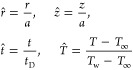 |
39 |
The concentrations and mass flow rates are scaled as follows
 |
40 |
 |
41 |
 |
42 |
| 43 |
The Marangoni-induced velocity is used to scale the velocity field inside the droplet. The thermal Marangoni number and the Marangoni-induced velocity are
| 44 |
| 45 |
In the binary mixture, the presence of ethanol concentration gradient introduces solutal capillary flow. The solutal Marangoni number and associated Marangoni-induced velocity are defined as follows
| 46 |
| 47 |
In addition to a more complete description of the model and COMSOL implementation, a comprehensive list of the important dimensionless numbers that govern gravitational, thermal, solutal, and evaporation effects in the droplet is given in ref (57). For the simulation parameters considered here, the relevant range of the dimensionless parameters is listed. Those numbers are estimated based on the values that have been chosen for the present study.
3. Results and Discussion
3.1. Validation
To validate the unified model for the binary mixture of ethanol–water, the volume fraction of our numerical simulation is compared against experimental and theoretical results of Gurrala et al.14 A test case with a = 1.35 [mm], h0 = 1.1 [mm], Tw = 333 [K], T∞ = 295 [K], θi = 78.3°, and RH = 36 and 18 wt% concentration of ethanol, which is the same as 20% volume concentration of ethanol case in ref (14),14 is simulated by our model. Figure 6 shows how the numerical simulation results compare to the experimental and theoretical results of ref (14). The root-mean-square error (RMSE) value for our model is 0.035 compared to the experimental volume fraction, and the value of the cross correlation is 0.99987, while the RMSE value for their theoretical model is 0.059 and the cross correlation is 0.98998. The comparison indicates that our results are in very good agreement with the experimental results, much better than their theoretical results. From the computational model, the calculated volume fraction (evaporation rate) agrees very well with the experimental data for the first half of nondimensional time (t/te ≤ 0.35), while it underpredicts the evaporation rate for the second half (t/te > 0.35). This may be due to the fact that only the diffusion equation is solved in the air subdomain. As a result, the concentration of ethanol and water vapor in air subdomain reaches a quasi-equilibrium state, which decreases the gradient, and therefore the evaporation rate, compared to the beginning of the process.
Figure 6.

Comparison of the nondimensional volume of the ethanol–water droplet as a function of nondimensional time (divided by the total time of evaporation) for experimental and theoretical results by14 and simulation results of our model for diffusion-only and diffusion with natural convection modes. Data for the experimental and theoretical profiles are adapted from Ref (14). Copyright 2019 with permission from Elsevier.
The temperature difference between the substrate and ambient is 38 [K], which leads the Rayleigh number to be in the range of 700–800 (at 314 [K]). This means that although the natural convection is not the dominant driving force affecting the concentration field, it cannot be ignored in this case. To simulate the natural convection in the air subdomain, the airflow field needs to be calculated. To do this, the compressible Navier–Stokes and continuity equations are solved for the air subdomain using the “Laminar Flow” module in COMSOL
| 48 |
| 49 |
where ρ is the density of air that varies with temperature and is automatically calculated by the “Non-Isothermal Flow” module in COMSOL that couples the "Heat Transfer" and "Laminar Flow" modules. The boundary conditions to solve eqs 48 and 49 are the no-slip (eq 50) at the substrate, slip condition at the droplet–air interface, and a pressure condition at the outlet (eq 51)
| 50 |
| 51 |
p0 is defined as the hydrostatic pressure
| 52 |
where ρ0 is the density of air at the ambient temperature.
The last step is to use the velocity field in the air subdomain to solve the convection–diffusion equation
| 53 |
| 54 |
The boundary conditions for solving the above-mentioned equations are the same as those for the diffusion equations (eqs 24, 25, 26, 30, and 31).
Figure 6 shows the nondimensional volume of the droplet for the model with natural convection included. The effect of including natural convection in the model reduces the differences between the simulation results and the experimental data over the period of evaporation. By adding natural convection, the RMSE value was reduced for the diffusion–convection model to 0.269 and the cross-correlation value improved to 0.99957.
Another effect that can contribute to the evaporation rate is the convection of ethanol vapor due to a large gradient of ethanol concentration between the droplet interface and the ambient boundary concentration. Calculating the evaporation rate due to convection requires a correlation to estimate the convective mass transfer coefficient. To the best of our knowledge, this type of correlation has only been developed for pure droplets.58 Theoretically, these correlations can be extended for the binary mixture droplets. However, since our diffusion-only model predicts the experimental data very well and we are considering lower ethanol concentrations, we did not include this contribution in the present model. This extension to the model could be considered in future work.
Since evaporation is the mechanism responsible for the volume loss and deriving the internal flow, good agreement in Figure 6 means the flow patterns should be similar.
Figures 7 and 8 show the concentration contours of ethanol vapor as [mol.m-3] in the air subdomain for the diffusion-only and diffusion with natural convection modes at 1[s] after the start of the process. It can be seen from the plots that in the diffusion-only mode, based on the solution to the Laplace equation, the concentration field is symmetric, while with the addition of natural convection, there is an upward velocity from the substrate that stretches the concentration field in the vertical direction and toward the apex of the droplet.
Figure 7.

Concentration contour of ethanol vapor as [mol.m-3] in the air subdomain for the diffusion-only mode at 1[s] from the beginning of the evaporation.
Figure 8.

Concentration contour of ethanol vapor as [mol.m-3]] in the air subdomain for the diffusion and natural convection modes at 1 [s] from the beginning of the evaporation.
3.2. Droplet Volume
The evaporation rate of the pure water droplet is approximately constant through evaporation time, which means that the volume of the droplet is decreasing linearly with time.7,8,15 In this section, the effect of the presence of the ethanol in the mixture on the rate of change of volume is investigated. The volume of the droplet is scaled by the radius of the droplet as follows
| 55 |
The time evolution of droplet volume is illustrated in Figure 9 for a mixture droplet with a 35wt% concentration of ethanol and initial contact angles of θi = 40, 60, and 80°. Ethanol is the more volatile component in the mixture since the concentration of ethanol vapor in air is zero at ambient conditions. At the first stage of evaporation, both water and ethanol evaporate simultaneously until the ethanol is completely evaporated. At the second stage, only the remaining water is evaporated. As a result, the rate of change of droplet volume is faster in the first stage and is approximately constant during the second stage (the same as the pure water case).
Figure 9.

Time evolution of the droplet volume of a binary mixture droplet with an initial concentration of 35 wt% ethanol and different initial contact angles of θi = 40, 60, and 80°.
3.3. Concentration Contours
Since the diffusion coefficient of ethanol in water is small (Dl,e = 1.5 × 10⁻⁹ [m2.s–1]), the diffusion Peclet number is much greater than 1 (PeD = UMga/Dl,e ≫ 1), which means that concentration distribution inside the droplet is dominated by solute convection. Velocity streamlines are depicted on top of the nondimensional concentration contours in Figure 10 for a mixture droplet with an initial concentration of 35% weight ethanol and an initial contact angle of θi = 40° at t̂ = 0.083, 0.167, and 0.25.
Figure 10.

Velocity streamlines on top of the nondimensional concentration contours for a mixture droplet with an initial concentration of 35% weight ethanol and an initial contact angle of θi = 40° at (a) t̂ = 0.083, (b) t̂ = 0.167, and (c) t̂ = 0.25.
At the beginning of the evaporation process, there is a uniform concentration of ethanol inside the mixture droplet. As soon as the Marangoni flow inside the droplet takes place, the concentration distribution mirrors the velocity field because of the convection-dominated process. Since the evaporation flux is the highest near the contact line, the concentration of solute is always minimum at the edge. The maximum concentration, on the other hand, is at the center of the vortex formed by the Marangoni convection, where some of the ethanol molecules become trapped. The velocity magnitude near the center of the vortex is very small, so the only way possible for ethanol molecules to escape is via diffusion, which is very weak. This fraction of ethanol molecules remain in the center of circular flow until the end of the first stage of evaporation in which the evaporation of ethanol is controlled by the diffusion of this small fraction toward the interface.35
3.4. Internal Flow Structure of Thermal and Solutal Marangoni Convection
The velocity field inside the droplet at the end of the first phase of evaporation (depinning process) mostly defines the deposition pattern upon drying. For binary mixture droplet, thermal Marangoni convection acts in the same way as the pure water droplet. The direction of thermal Marangoni flow is always outward near the substrate and inward near the interface. In this section, we introduce solutal Marangoni convection to the system as a result of concentration gradient on the interface. It is shown in Figure 10 that the concentration of solute is minimum at the contact line (because of the highest evaporative flux) while it obtains its maximum value near the top of the drop. Surface tension of water decreases by an increase in ethanol concentration. Therefore, surface tension is lower at the apex and is higher at the contact line. The direction of Marangoni stress is always from the lower surface tension to higher surface tension, so solutal Marangoni flow is outward near the interface and inward close to the substrate (reverse direction of thermal Marangoni). Competition between thermal and solutal Marangoni defines the velocity field inside the droplet.
Thermal and solutal Marangoni numbers are defined in eqs 44 and 46. We are utilizing these two nondimensional numbers to determine the dominant Marangoni flow direction. If Mgs > MgT, solutal Marangoni is dominant and flow direction is from the apex of the droplet toward the contact line and vice versa. To scale the velocity field, the Marangoni-induced velocity is defined as follows
| 56 |
To show the general evaporation dynamics of a binary mixture droplet, we simulate an ethanol–water droplet with a = 1.3 [mm] and h0 = 0.46 [mm], Tw = T∞ = 299 [K], θi = 36°, and RH = 50% (same condition as Kim et al.59). The only difference between our model and their experiments is that we did not consider the effect of surfactant in our model.
Three general stages of evaporation in ethanol–water droplet are shown in Figure 11. In the first stage, which develops at early evaporation time, several random vortices are formed inside the droplet as a result of local concentration gradients. These local concentration gradients have a significant effect in producing local surface tension gradients and as a result local vortices. The presence of these multiple vortices has been observed by Kim et al.59 and Hamamoto et al.38 As the droplet evaporates, the concentration of ethanol near the contact line becomes lower than that of the droplet apex due to nonuniform evaporative flux. As a result, we have a strong solutal Marangoni stress acting on the interface toward the contact line, which creates an outward velocity near the droplet surface. During this stage, solutal Marangoni is dominant over thermal Marangoni. Finally, in the third stage, the ethanol evaporates, completely eliminating the solutal Marangoni stress. During the last stage, thermal Marangoni takes over the system and the flow pattern is similar to the pure water droplet (inward velocity near the interface).
Figure 11.

Three stages of evaporation for an ethanol–water droplet with a = 1.3 [mm] and h0 = 0 46 [mm],Tw = T∞ = 299 [K], θi = 36°, and RH = 50% at (a) t = 0.5 [s], (b) t = 90 [s], and (c) t = 205 [s].
To investigate the deposition pattern of an ethanol–water droplet, we evaluated all cases at the time of evaporation for which the contact angle is 15°. The influence of initial ethanol concentration on the velocity field inside the drop has been studied. All results presented here are contours of nondimensional velocity magnitude and velocity vectors.
The effect of initial ethanol concentration (solutal Marangoni number) is demonstrated in Figure 12. The results presented here are for droplets with an initial contact angle of θi = 40° at t̂ = 0.5 on the substrate with a temperature of Tw = 298 [K] with initial ethanol concentrations of 5, 20, and 35 wt%. The thermal and solutal Marangoni numbers and the Marangoni-induced velocity are MgS = 0, 61 525, and 125 725, MgT = 236, 186, and 161, and UMg = 0.032, 0.086, and 0.176 [m·s–1], respectively. These values show that at 5 wt% initial concentration, ethanol is totally evaporated before the end of the simulation. Therefore, there is no longer solutal Marangoni convection and thermal Marangoni flow dominates, so the direction of Marangoni flow is inward near the interface.
Figure 12.

Effect of initial ethanol concentrations on the velocity field inside the isothermal droplet with an initial contact angle of θi = 40° for (a) 5 wt%, MgS = 0, MgT = 236, UMg = 0.032 [m·s–1], (b) 20 wt%, MgS = 61525, MgT = 186, UMg = 0.086 [m·s–1], and (c) 35 wt%, MgS = 125 725, MgT = 161, UMg = 0.176 [m·s–1].
The temperature difference between the top and the edge of the droplet is lower for higher initial ethanol concentration. The evaporative cooling effect on the interface is the sum of the evaporative cooling effect of both ethanol and water. At higher initial ethanol concentration, the evaporation rate of water (evaporation cooling effect) is higher and the evaporation rate of ethanol is lower than the case of lower initial ethanol concentration (for the case with 5 wt%, the evaporation cooling is the same as pure water). Since the latent heat of water is much larger than that of ethanol, evaporative cooling is increased by a decrease in initial ethanol concentration, which generates a greater temperature difference.
For two cases with initial ethanol concentrations of 20 and 35 wt%, the solutal Marangoni number is much higher than the thermal Marangoni number by at least 2 orders of magnitude. Therefore, the direction of Marangoni convection inside the droplet is outward near the interface and inward near the substrate. This flow suppresses the capillary flow, which is the main reason for the formation of the coffee ring.
The velocity magnitude plots demonstrate greater velocity magnitude for the case with 35 wt% ethanol. The evaporation rate of ethanol is higher for greater values of initial ethanol concentrations. Therefore, the gradient of concentration is greater between the contact line and the apex, which leads to a greater solutal Marangoni number.
Potentially, solutal Marangoni flow can prevent the formation of the coffee ring. However, this would require that all of the ethanol does not evaporate before the end of the evaporation process. In order for this to be the case, higher initial ethanol concentration and lower initial contact angle are required. In the simulation results, the droplet with a greater initial contact angle needs more time to evaporate (t̂ = 2 and 0.75 for a droplet with initial contact angles of θi = 80° and 40°, respectively). The longer evaporation time provides the opportunity for the ethanol to completely evaporate before reaching the point when deposition starts. Therefore, based on the cases simulated, more uniform deposition is obtained for the case with θi = 40° and 35 wt% of initial ethanol concentration.
4. Conclusions
Numerical simulations were used to quantify the evaporation rate and internal flow structure of sessile droplets of a binary fluid on heated, isothermal substrates. For the properties of the ethanol–water system, simulations have been performed for droplets with different initial contact angles and thermal and solutal Marangoni numbers. The effect on the velocity field inside the droplet was investigated.
In the case of binary mixture droplets for the temperature range considered, solutal Marangoni convection always dominates the thermal Marangoni-driven flow and creates an outward flow near the interface. Higher initial ethanol concentration results in greater solutal capillary convection. Also, solutal Marangoni flow can suppress the basic capillary flow and prevent the formation of the coffee ring. All of this behavior exists before ethanol inside the drop completely evaporates. The simulation results yield guidance for processing conditions for the system studied; for example, more uniform deposition is obtained for an ethanol–water binary droplet with an initial contact angle of θi = 40° and an initial ethanol concentration of 35 wt% or higher.% or higher.
The authors declare no competing financial interest.
References
- Dugas V.; Broutin J.; Souteyrand E. Droplet evaporation study applied to DNA chip manufacturing. Langmuir 2005, 21, 9130–9136. 10.1021/la050764y. [DOI] [PubMed] [Google Scholar]
- Ortiz C.; Zhang D.; Xie Y.; Ribbe A. E.; Ben-Amotz D. Validation of the drop coating deposition Raman method for protein analysis. Anal. Biochem. 2006, 353, 157–166. 10.1016/j.ab.2006.03.025. [DOI] [PubMed] [Google Scholar]
- Filik J.; Stone N. Drop coating deposition Raman spectroscopy of protein mixtures. Analyst 2007, 132, 544–550. 10.1039/b701541k. [DOI] [PubMed] [Google Scholar]
- Jia W.; Qiu H.-H. Experimental investigation of droplet dynamics and heat transfer in spray cooling. Exp. Therm. Fluid Sci. 2003, 27, 829–838. 10.1016/S0894-1777(03)00015-3. [DOI] [Google Scholar]
- Brinker C. J.; Lu Y.; Sellinger A.; Fan H. Evaporation-induced self-assembly: nanostructures made easy. Adv. Mater. 1999, 11, 579–585. 10.1002/(sici)1521-4095(199905)11:73.0.co;2-r. [DOI] [Google Scholar]
- Marín Á. G.; Gelderblom H.; Lohse D.; Snoeijer J. H. Order-to-disorder transition in ring-shaped colloidal stains. Phys. Rev. Lett. 2011, 107, 085502 10.1103/PhysRevLett.107.085502. [DOI] [PubMed] [Google Scholar]
- Picknett R.; Bexon R. The evaporation of sessile or pendant drops in still air. J. Colloid Interface Sci. 1977, 61, 336–350. 10.1016/0021-9797(77)90396-4. [DOI] [Google Scholar]
- Hu H.; Larson R. G. Evaporation of a sessile droplet on a substrate. J. Phys. Chem. B 2002, 106, 1334–1344. 10.1021/jp0118322. [DOI] [Google Scholar]
- Birdi K.; Vu D.; Winter A. A study of the evaporation rates of small water drops placed on a solid surface. J. Phys. Chem. A 1989, 93, 3702–3703. 10.1021/j100346a065. [DOI] [Google Scholar]
- Yu H.-Z.; Soolaman D. M.; Rowe A. W.; Banks J. T. Evaporation of Water Microdroplets on Self-Assembled Monolayers: From Pinning to Shrinking. ChemPhysChem 2004, 5, 1035–1038. 10.1002/cphc.200301042. [DOI] [PubMed] [Google Scholar]
- Bourges-Monnier C.; Shanahan M. Influence of evaporation on contact angle. Langmuir 1995, 11, 2820–2829. 10.1021/la00007a076. [DOI] [Google Scholar]
- Rowan S. M.; Newton M.; McHale G. Evaporation of microdroplets and the wetting of solid surfaces. J. Phys. Chem. A 1995, 99, 13268–13271. 10.1021/j100035a034. [DOI] [Google Scholar]
- Gleason K.; Voota H.; Putnam S. A. Steady-state droplet evaporation: Contact angle influence on the evaporation efficiency. Int. J. Heat Mass Transfer 2016, 101, 418–426. 10.1016/j.ijheatmasstransfer.2016.04.075. [DOI] [Google Scholar]
- Gurrala P.; Katre P.; Balusamy S.; Banerjee S.; Sahu K. C. Evaporation of ethanol-water sessile droplet of different compositions at an elevated substrate temperature. Int. J. Heat Mass Transfer 2019, 145, 118770 10.1016/j.ijheatmasstransfer.2019.118770. [DOI] [Google Scholar]
- Langmuir I. The evaporation of small spheres. Phys. Rev. 1918, 12, 368. 10.1103/PhysRev.12.368. [DOI] [Google Scholar]
- Silverman R. A.Special Functions and Their Applications; Courier Corporation: 1972; pp 1–308. [Google Scholar]
- Schönfeld F.; Graf K.-H.; Hardt S.; Butt H.-J. Evaporation dynamics of sessile liquid drops in still air with constant contact radius. Int. J. Heat Mass Transfer 2008, 51, 3696–3699. 10.1016/j.ijheatmasstransfer.2007.12.027. [DOI] [Google Scholar]
- Deegan R. D.; Bakajin O.; Dupont T. F.; Huber G.; Nagel S. R.; Witten T. A. Capillary flow as the cause of ring stains from dried liquid drops. Nature 1997, 389, 827. 10.1038/39827. [DOI] [Google Scholar]
- Deegan R. D. Pattern formation in drying drops. Phys. Rev. E 2000, 61, 475. 10.1103/PhysRevE.61.475. [DOI] [PubMed] [Google Scholar]
- Wang T.-S.; Shi W.-Y. Transition of Marangoni convection instability patterns during evaporation of sessile droplet at constant contact line mode. Int. J. Heat Mass Transfer 2020, 148, 119138 10.1016/j.ijheatmasstransfer.2019.119138. [DOI] [Google Scholar]
- Ye S.; Zhang L.; Wu C.-M.; Li Y.-R.; Liu Q.-S. Experimental investigation on evaporation dynamics of sessile ethanol droplets on a heated substrate. Int. J. Heat Mass Transfer 2020, 162, 120352 10.1016/j.ijheatmasstransfer.2020.120352. [DOI] [Google Scholar]
- Xu X.; Luo J. Marangoni flow in an evaporating water droplet. Appl. Phys. Lett. 2007, 91, 124102 10.1063/1.2789402. [DOI] [Google Scholar]
- Zhang Y.; Zhang L.; Mo D.-M.; Wu C.-M.; Li Y.-R. Numerical investigation on flow instability of sessile ethanol droplets evaporating in its pure vapor at low pressure. Int. J. Heat Mass Transfer 2020, 156, 119893 10.1016/j.ijheatmasstransfer.2020.119893. [DOI] [Google Scholar]
- Girard F.; Antoni M.; Faure S.; Steinchen A. Evaporation and Marangoni driven convection in small heated water droplets. Langmuir 2006, 22, 11085–11091. 10.1021/la061572l. [DOI] [PubMed] [Google Scholar]
- Girard F.; Antoni M.; Sefiane K. On the effect of Marangoni flow on evaporation rates of heated water drops. Langmuir 2008, 24, 9207–9210. 10.1021/la801294x. [DOI] [PubMed] [Google Scholar]
- Lu G.; Duan Y.-Y.; Wang X.-D.; Lee D.-J. Internal flow in evaporating droplet on heated solid surface. Int. J. Heat Mass Transfer 2011, 54, 4437–4447. 10.1016/j.ijheatmasstransfer.2011.04.039. [DOI] [Google Scholar]
- Chen Y.; Hong F.; Cheng P. Transient flow patterns in an evaporating sessile drop: A numerical study on the effect of volatility and contact angle. Int. Commun. Heat Mass Transfer 2020, 112, 104493 10.1016/j.icheatmasstransfer.2020.104493. [DOI] [Google Scholar]
- Semenov S.; Carle F.; Medale M.; Brutin D. 3D unsteady computations of evaporative instabilities in a sessile drop of ethanol on a heated substrate. Appl. Phys. Lett. 2017, 111, 241602 10.1063/1.5006707. [DOI] [PubMed] [Google Scholar]
- Barmi M. R.; Meinhart C. D. Convective flows in evaporating sessile droplets. J. Phys. Chem. B 2014, 118, 2414–2421. 10.1021/jp408241f. [DOI] [PubMed] [Google Scholar]
- Hu H.; Larson R. G. Analysis of the effects of Marangoni stresses on the microflow in an evaporating sessile droplet. Langmuir 2005, 21, 3972–3980. 10.1021/la0475270. [DOI] [PubMed] [Google Scholar]
- Hu H.; Larson R. G. Analysis of the microfluid flow in an evaporating sessile droplet. Langmuir 2005, 21, 3963–3971. 10.1021/la047528s. [DOI] [PubMed] [Google Scholar]
- Chen X.; Wang X.; Chen P. G.; Liu Q. Thermal effects of substrate on Marangoni flow in droplet evaporation: response surface and sensitivity analysis. Int. Commun. Heat Mass Transfer 2017, 113, 354–365. 10.1016/j.ijheatmasstransfer.2017.05.076. [DOI] [Google Scholar]
- Rowan S.; Newton M.; Driewer F.; McHale G. Evaporation of microdroplets of azeotropic liquids. J. Phys. Chem. B 2000, 104, 8217–8220. 10.1021/jp000938e. [DOI] [Google Scholar]
- Christy J. R.; Sefiane K.; Munro E. A study of the velocity field during evaporation of sessile water and water/ethanol drops. J. Bionic Eng. 2010, 7, 321–328. 10.1016/S1672-6529(10)60263-6. [DOI] [Google Scholar]
- Liu C.; Bonaccurso E.; Butt H.-J. Evaporation of sessile water/ethanol drops in a controlled environment. Phys. Chem. Chem. Phys. 2008, 10, 7150–7157. 10.1039/b808258h. [DOI] [PubMed] [Google Scholar]
- Sefiane K. On the Dynamic Capillary Effects in the Wetting and evaporation process of Binary Droplets. Fluid Dyn. Mater. Process. 2005, 1, 267–276. [Google Scholar]
- Cheng A. K.; Soolaman D. M.; Yu H.-Z. Evaporation of Microdroplets of Ethanol- Water Mixtures on Gold Surfaces Modified with Self-Assembled Monolayers. J. Phys. Chem. B 2006, 110, 11267–11271. 10.1021/jp0572885. [DOI] [PubMed] [Google Scholar]
- Hamamoto Y.; Christy J. R.; Sefiane K. The flow characteristics of an evaporating ethanol water mixture droplet on a glass substrate. J. Therm. Sci. Technol. 2012, 7, 425–436. 10.1299/jtst.7.425. [DOI] [Google Scholar]
- Talbot E.; Berson A.; Bain C.. Drying and Deposition of Picolitre Droplets of Colloidal Suspensions in Binary Solvent Mixtures. In NIP & Digital Fabrication Conference, 2012; pp 420–423.
- Talbot E.; Berson A.; Yang L.; Bain C.. Internal Flows and Particle Transport Inside Picoliter Droplets of Binary Solvent Mixtures. In NIP & Digital Fabrication Conference, 2013; pp 307–312.
- Diddens C.; Kuerten J. G.; Van der Geld C.; Wijshoff H. Modeling the evaporation of sessile multi-component droplets. J. Colloid Interface Sci. 2017, 487, 426–436. 10.1016/j.jcis.2016.10.030. [DOI] [PubMed] [Google Scholar]
- Diddens C. Detailed finite element method modeling of evaporating multi-component droplets. J. Comput. Phys. 2017, 340, 670–687. 10.1016/j.jcp.2017.03.049. [DOI] [Google Scholar]
- Diddens C.; Tan H.; Lv P.; Versluis M.; Kuerten J.; Zhang X.; Lohse D.. Evaporating pure, binary and ternary droplets: thermal effects and axial symmetry breaking 2017, arXiv:1706.06874. arXiv.org e-preprint. archieve. https://arxiv.org/abs/1706.06874.
- Yunker P. J.; Still T.; Lohr M. A.; Yodh A. Suppression of the coffee-ring effect by shape-dependent capillary interactions. Nature 2011, 476, 308–311. 10.1038/nature10344. [DOI] [PubMed] [Google Scholar]
- Cui L.; Zhang J.; Zhang X.; Huang L.; Wang Z.; Li Y.; Gao H.; Zhu S.; Wang T.; Yang B. Suppression of the coffee ring effect by hydrosoluble polymer additives. ACS Appl. Mater. Interfaces 2012, 4, 2775–2780. 10.1021/am300423p. [DOI] [PubMed] [Google Scholar]
- Crivoi A.; Duan F. Elimination of the coffee-ring effect by promoting particle adsorption and long-range interaction. Langmuir 2013, 29, 12067–12074. 10.1021/la402544x. [DOI] [PubMed] [Google Scholar]
- Crivoi A.; Duan F. Three-dimensional Monte Carlo model of the coffee-ring effect in evaporating colloidal droplets. Sci. Rep. 2014, 4, 4310 10.1038/srep04310. [DOI] [PMC free article] [PubMed] [Google Scholar]
- Li Y.; Yang Q.; Li M.; Song Y. Rate-dependent interface capture beyond the coffee-ring effect. Sci. Rep. 2016, 6, 27963 10.1038/srep27963. [DOI] [PMC free article] [PubMed] [Google Scholar]
- Bhardwaj R.; Fang X.; Somasundaran P.; Attinger D. Self-assembly of colloidal particles from evaporating droplets: role of DLVO interactions and proposition of a phase diagram. Langmuir 2010, 26, 7833–7842. 10.1021/la9047227. [DOI] [PubMed] [Google Scholar]
- COMSOL Microfluidics Module User’s Guide v. 5.2. COMSOL Multiphysics: COMSOL AB; Stockholm, Sweden, 2016. [Google Scholar]
- Vazquez G.; Alvarez E.; Navaza J. M. Surface tension of alcohol water+ water from 20 to 50. degree. C. J. Chem. Eng. Data 1995, 40, 611–614. 10.1021/je00019a016. [DOI] [Google Scholar]
- Perrot P.A to Z of Thermodynamics; Oxford University Press on Demand, 1998; pp 1–329. [Google Scholar]
- Bennacer R.; Sefiane K. Vortices, dissipation and flow transition in volatile binary drops. J. Fluid Mech. 2014, 749, 649–665. 10.1017/jfm.2014.220. [DOI] [Google Scholar]
- Wang J.-F.; Li C.-X.; Wang Z.-H.; Li Z.-J.; Jiang Y.-B. Vapor pressure measurement for water, methanol, ethanol, and their binary mixtures in the presence of an ionic liquid 1-ethyl-3-methylimidazolium dimethylphosphate. Fluid Phase Equilib. 2007, 255, 186–192. 10.1016/j.fluid.2007.04.010. [DOI] [Google Scholar]
- Thomson G. W. The Antoine equation for vapor-pressure data. Chem. Rev. 1946, 38, 1–39. 10.1021/cr60119a001. [DOI] [PubMed] [Google Scholar]
- Khattab I. S.; Bandarkar F.; Fakhree M. A. A.; Jouyban A. Density, viscosity, and surface tension of water+ ethanol mixtures from 293 to 323K. Korean J. Chem. Eng. 2012, 29, 812–817. 10.1007/s11814-011-0239-6. [DOI] [Google Scholar]
- Bozorgmehr B.Evaporation of Pure Water And Ethanol-water Mixture Droplets on Isothermal and Heated Substrates, A Numerical Approach; State University of New York at Binghamton, 2016; pp 1–60. [Google Scholar]
- Kelly-Zion P.; Pursell C. J.; Wassom G. N.; Mandelkorn B. V.; Nkinthorn C. Correlation for sessile drop evaporation over a wide range of drop volatilities, ambient gases and pressures. Int. J. Heat Mass Transfer 2018, 118, 355–367. 10.1016/j.ijheatmasstransfer.2017.10.129. [DOI] [Google Scholar]
- Kim H.; Boulogne F.; Um E.; Jacobi I.; Button E.; Stone H. A. Controlled uniform coating from the interplay of Marangoni flows and surface-adsorbed macromolecules. Phys. Rev. Lett. 2016, 116, 124501 10.1103/PhysRevLett.116.124501. [DOI] [PubMed] [Google Scholar]