Effect of Water Content on Thermodynamic Properties of Compressed Hydrogen

Abstract

Force field-based molecular simulations were used to calculate thermal expansivities, heat capacities, and Joule–Thomson coefficients of binary (standard) hydrogen–water mixtures for temperatures between 366.15 and 423.15 K and pressures between 50 and 1000 bar. The mole fraction of water in saturated hydrogen–water mixtures in the gas phase ranges from 0.004 to 0.138. The same properties were calculated for pure hydrogen at 323.15 K and pressures between 100 and 1000 bar. Simulations were performed using the TIP3P and a modified TIP4P force field for water and the Marx, Vrabec, Cracknell, Buch, and Hirschfelder force fields for hydrogen. The vapor–liquid equilibria of hydrogen–water mixtures were calculated along the melting line of ice Ih, corresponding to temperatures between 264.21 and 272.4 K, using the TIP3P force field for water and the Marx force field for hydrogen. In this temperature range, the solubilities and the chemical potentials of hydrogen and water were obtained. Based on the computed solubility data of hydrogen in water, the freezing-point depression of water was computed ranging from 264.21 to 272.4 K. The modified TIP4P and Marx force fields were used to improve the solubility calculations of hydrogen–water mixtures reported in our previous study [Rahbari A.;et al. J. Chem. Eng. Data 2019, 64, 4103−4115] for temperatures between 323 and 423 K and pressures ranging from 100 to 1000 bar. The chemical potentials of ice Ih were calculated as a function of pressure between 100 and 1000 bar, along the melting line for temperatures between 264.21 and 272.4 K, using the IAPWS equation of state for ice Ih. We show that at low pressures, the presence of water has a large effect on the thermodynamic properties of compressed hydrogen. Our conclusions may have consequences for the energetics of a hydrogen refueling station using electrochemical hydrogen compressors.

1. Introduction

To supply the energy demand for a growing population worldwide and to reduce carbon emissions, efforts are being made to switch from fossil-based energy production to sustainable energy production using renewable energy sources.¹⁻⁵ Current estimations show that in 2050 ca. 75% of the global energy production will be based on fossil fuels.¹ In recent years, hydrogen is considered as one of the most promising alternatives in the energy transition for combating global warming and reducing the carbon footprint from anthropogenic activities.^4,6−11 Hydrogen is one of the most abundant elements found on earth mainly in water and organic compounds.³ To produce hydrogen as a free gas, energy is required.^2,12 Hydrogen can be a carbon-free renewable energy source depending on the production pathway,¹²e.g., green hydrogen can be produced from water electrolysis in which the required energy is supplied from renewable sources. The high energy density of hydrogen per unit of mass (higher heating value of 141.8 MJ/kg at 298 K)¹² makes it a flexible off-peak energy carrier, especially for storing intermittent renewable energy at peak times, or as a fuel for transportation.^6,13−15 To date, most of the required hydrogen in refineries is produced from steam methane reforming (SMR) with CO₂ as a byproduct.^2,4,8,12,16 About 50% of the produced hydrogen worldwide is used in ammonia synthesis plants. Hydrogen is also used as a hydrocarbon upgrader or feedstock in refineries, e.g., reducing nitrogen oxides, sulfur oxides, and other particles causing smog.^6,17

The heating value of hydrogen (per mass) is higher than that of most common fossil fuels.^2,12 However, due to the low volumetric density of hydrogen at standard temperature and pressure, 273.15 K and 1 bar (10.79 MJ/m³),⁹ and to save space, gaseous hydrogen should be compressed, liquefied, or absorbed by metal hydrides or nanoporous materials such as metal–organic frameworks (MOFs).^{2,3,7,17−19} Compressing hydrogen increases the heating value (per unit of volume) compared to the heating value of conventional liquid fossil fuels.¹² Compressed hydrogen can be used in fuel-cell electric vehicles or hydrogen-fueled combustion engines.^1,17,20 To facilitate and increase the use of hydrogen-driven vehicles, hydrogen refueling stations (HRSs) should provide compressed hydrogen to fuel-cell electric vehicles or internal combustion hydrogen engines.²¹ Current vehicle technologies allow direct on-board hydrogen storage with pressures up to 700 bar inside the tank.^{9,18,20,22,23} This allows a driving range of at least 500 km.^1,9,24−26 To meet the target refueling time (3–4 min),^22,23 a large pressure difference is required when filling the hydrogen tank, e.g., the pressure of compressed hydrogen before entering the vehicle should be as high as 875 bar.²¹ Therefore, energy- and cost-efficient hydrogen compression technologies are required for operating refueling stations at these high pressures.

Hydrogen compression technologies can be divided into mechanical and nonmechanical categories.⁹ There are well-known limitations associated with mechanical compression such as high mechanical losses, high maintenance, high levels of noise, etc.²⁰ In addition, the compression work can be as high as 30% of the energy of the stored hydrogen,²⁷ and the efficiency is low when operating at small scales.^9,28 Alternatives to mechanical compression are (1) cryogenic compression, (2) metal hydride or thermally powered compressors,²⁹ and (3) electrochemical hydrogen compressors (EHCs), also known as electrochemical hydrogen pumps.^9,20,30 A detailed overview of conventional and state-of-the-art technologies for hydrogen compression technologies is provided in ref (9).

Recently, EHCs have become cost-competitive alternatives to their mechanical counterparts.^16,30,31 Due to the advantages over mechanical compression, EHCs are on the way to be commercialized on a large scale. EHCs can generate a high output pressure (up to 1000 bar), which is suitable for refueling hydrogen vehicles.^20,30 EHCs have a higher efficiency compared to mechanical compression, especially for low volumetric flows.^9,32 Since there are no moving parts in an EHC, there are no maintenance costs associated with rotary parts, and the compressor operates silently. The working principle of an EHC is based on the proton-exchange membrane fuel-cell technology.^4,9,30 A schematic representation of the working principle of an EHC is shown in Figure 1. On the anode side, electricity is used to split the hydrogen molecule into protons and electrons, and the protons pass through the membrane. Hydrated protons (H_2n+1O_n⁺ in which n is the electro-osmosis coefficient) are transferred to the cathode side.^4,9,13 At the cathode side, the protons are combined with electrons to form hydrogen molecules.²⁰ As the number of hydrogen molecules increases on the cathode side, the discharge pressure at the outlet of the EHC increases. In EHCs, the driving force for compression is the electrical potential difference between the anode and the cathode. This means that the discharge pressure can be as large as allowed by material limitations. It is important to note that generating a large differential pressure over a single compression cell lowers the efficiency of the EHC and may cause back-diffusion of hydrogen from the cathode to the anode side.^9,20 To circumvent this issue, one can raise the discharge pressure using a cascaded arrangement of single compression cells.^30,33 The highest differential pressure reported in the literature for a single compression cell is 168 bar.²⁰ Two types of proton conducting membranes are typically used for electrochemical compression:¹⁶¹⁶ (1) proton electrolyte membranes such as Nafion-type membranes,^16,28,34 which are suitable for low-temperature applications; and (2) protonic-ceramic electrolyte membranes, which are suitable for high-temperature applications (e.g., 600 °C).¹⁶ These membranes are highly selective to permeation of protons as impurities cannot pass the membrane.³³ The proton-exchange membrane requires hydration for its functionality. Therefore, it is important that the membrane inside the compressor remains hydrated with water when operating. While compressing the hydrogen stream, the EHC can simultaneously purify the hydrogen stream such that the compressed hydrogen at the outlet is saturated with water, and no other impurities are present. Recently, HyET BV^30,31 has developed state-of-the-art EHCs operating based on the proton-exchange membrane technology. Currently, each compression stack can compress 50 kg H₂/day up to 1000 bar. The EHC capacity can be scaled up using several compression stacks.^31,33 The EHC by HyET BV can achieve the same pressure difference as in mechanical compression with fewer steps and silently. The compressed hydrogen is saturated with water and free from other contaminants.

Figure 1.

Schematic representation of the working principle of electrochemical compression of hydrogen.³⁰ Hydrogen molecules are split at the low-pressure side of the membrane (i.e., using platinum-alloy catalysts). Protons are forced through the membrane and form hydrogen molecules at the high-pressure side.

Here, we consider the application of an EHC to generate compressed hydrogen for refueling a hydrogen vehicle. Although the solubility of water in compressed hydrogen at the outlet of the EHC is very low, this affects the thermodynamic behavior of the gas phase (depending on the water content). As the compressed hydrogen gas enters the on-board storage tank, it follows directly from the first law of thermodynamics of an open system that the temperature of hydrogen inside the tank rises. A similar effect happens for the isenthalpic expansion of hydrogen (e.g., using a throttle) due to the negative Joule–Thomson coefficient of hydrogen at high pressures.^23,35 To protect the mechanical integrity of the tank, the maximum temperature limit of the hydrogen in the process of filling should not exceed 85 °C.^26,35,36 To avoid high temperatures inside the hydrogen tank, precooling is required before refueling to bring the temperature of compressed hydrogen down between −33 and −40 °C.^23,26,35 A complete hydrogen fueling protocol is compiled by the Society of Automotive Engineers (SAE) in “Fueling Protocols for Light Duty Gaseous Hydrogen Surface Vehicles (SAE J2601)”.^22,37

Due to the presence of water content at the output of an EHC, ice formation may take place during precooling, which may clog the hydrogen delivery system. Experimental data on the solubility and other thermodynamic properties of water–hydrogen systems in the published literature are limited, especially at high pressures.^38,39 Published experimental data for solubilities of water–hydrogen mixtures in the gas or/and liquid phase at high pressures can be found in refs (40−49). A summary of the experimental data in the tabulated form can be found in ref (38). However, little is known about the influence of water on the thermodynamic properties of hydrogen at high pressures. Performing experiments for obtaining thermodynamic data at high pressures is challenging due to safety protocols, material limitations, high costs, etc.⁵⁰⁻⁵⁴ A robust alternative for high-pressure experiments is force-field-based molecular simulation.^55,56 In this work, we use force-field-based molecular simulation to calculate properties of compressed hydrogen by varying the water content at different temperatures and pressures. Molecular simulation is an approach for calculating macroscopic as well microscopic properties of materials based on the knowledge of their constituent molecules and atoms as well as their interactions. Molecular simulation allows the computation of material properties at high pressures, which would be difficult or expensive to access using experiments. By modeling the VLE of water–hydrogen systems, it is possible to compute the amount of water present in compressed hydrogen at temperatures and pressures corresponding to the freezing point of water. In this way, one can predict water/ice formation when precooling the hydrogen stream. The VLE calculations can also be used to predict the freezing-point depression of water in the presence of hydrogen. In this work, the VLE calculations of hydrogen–water are performed at temperatures and pressures corresponding to the water–ice Ih equilibrium in the pressure range between 100 and 1000 bar. Using molecular simulation, we also calculate thermodynamic properties such as thermal expansivity, heat capacity, and the Joule–Thomson coefficient of the water–hydrogen mixtures.

This paper is organized as follows. Thermodynamic properties of compressed hydrogen–water mixtures are investigated using force-field-based molecular simulation. An overview of the molecular models used in this paper is provided in Table 1. Thermodynamic properties of mixtures are related to the derivatives of extensive properties of the mixtures.⁵⁷ One can calculate the appropriate thermodynamic derivatives (i.e., for calculating heat capacities, thermal expansivities, and Joule–Thomson coefficients) from ensemble fluctuations.^55,56,58 In Section 2, we provide the appropriate expressions for calculating thermodynamic derivatives to obtain the required thermodynamic properties. In Section 3, we explain how vapor–liquid equilibria of hydrogen–water mixtures along the melting line of ice can be computed. This allows one to estimate how much water would exit the saturated hydrogen stream during deep cooling at low temperatures. To the best of our knowledge, high-pressure experimental data of water–hydrogen systems at temperatures between 264.2 and 272.4 K are not available in the literature. Volumetric data from the literature are used to compute the chemical potential of ice for a large pressure range. Simulation details are provided in Section 4. All simulation results are presented and discussed in Section 5. Our conclusions are summarized in Section 6. The results show that small concentrations of water dissolved in hydrogen in the gas phase can significantly change the properties of the gas phase (i.e., Joule–Thomson coefficient, heat capacity, and thermal expansivity) compared to pure hydrogen at the same conditions. Our results will therefore have consequences for the energetics of a hydrogen refueling station using EHCs including drying or precooling of the compressed hydrogen stream.

Table 1. Chemical Compounds Used for Molecular Simulation in This Work^a.

chemical name	chemical formula	CAS number	force field
water	H2O	7732-18-5	TIP3P100
water	H2O	7732-18-5	modified TIP4P (this work)
hydrogen	H2	1333-74-0	Marx99
hydrogen	H2	1333-74-0	Vrabec102
hydrogen	H2	1333-74-0	Cracknell97
hydrogen	H2	1333-74-0	Hirschfelder107
hydrogen	H2	1333-74-0	Buch106

^aFor direct computation of chemical potentials, improving the efficiency, and calculating the solubilites, fractional molecules are used. Interaction parameters of the modified TIP4P force field are provided in the Supporting Information (SI). Mixture compositions of water−hydrogen systems are explicitly provided for every temperature and pressure in Table 2.

2. Thermodynamic Properties of Mixtures Obtained from Ensemble Fluctuations

To compute thermodynamic properties of compressed hydrogen with and without traces of water using molecular simulations, we use derivatives of volume, internal energy, and enthalpy with respect to temperature and pressure. These derivatives are required to calculate properties such as thermal expansivity, heat capacity, and the Joule–Thomson coefficient.^57,59,60 These thermodynamic derivatives are directly obtained from ensemble fluctuations at constant composition.^56,58,61,62 Lagache et al.⁵⁸ showed that the derivative of an extensive property X with respect to β = 1/(k_BT) (in which k_B is the Boltzmann constant and T the absolute temperature) in the NPT ensemble can be obtained from the ensemble fluctuations as follows

1

where Ĥ = U + PV is the configurational enthalpy of the system,⁵⁸P is the imposed pressure, and U is the potential energy of the system consisting of an intermolecular contribution U^ext and an intramolecular contribution U^int. The mathematical proof for this is provided in the Supporting Information. In a similar manner, one can obtain an expression for the derivative of the ensemble average of an extensive property X with respect to pressure⁵⁸

2

The last term on the right-hand side of eq 2 is nonzero if the extensive property X includes a pressure-dependent contribution, for instance, for the configurational enthalpy Ĥ. The term was not explicitly provided in the corresponding equation in ref (58). The derivation of eq 2 is also provided in the Supporting Information. The extensive property X may be replaced by an intensive property x. Using eqs 1 and 2, one can obtain various thermodynamic properties of mixtures from ensemble fluctuations. For instance, combining the definition of thermal expansivity α_P with eq 2(58) leads to

3

To compute the Joule–Thomson coefficient, one needs to compute the heat capacity of the mixture as well. The extensive heat capacity follows from combining the definition of the heat capacity with eq 1

4

where the enthalpy H also includes the kinetic energy term (K): H = U^int + U^ext + K + PV = Ĥ + K. Jorgensen et al.⁶³ and Lagache et al.⁵⁸ emphasize that the expression for the heat capacity should be split into an ideal contribution and a residual contribution.

5

Including the ideal gas contribution of heat capacity from the force field usually leads to overestimating the heat capacity.^64,65 To calculate C_P^id(T) and C_P(T, P), Lagache et al.⁵⁸ proposed the following split for the enthalpy of the system

6

in which N is the number of molecules in the systems. The ideal gas heat capacity for a pure component can be obtained from tabulated thermodynamic reference tables.^59,66 Alternatively, C_P^id can be calculated by taking into account the contribution of translational, rotational, vibrational, and electronic energy levels of an isolated molecule, using quantum mechanical calculations or experimental data.^67,68 The residual heat capacity C_P is obtained by combining eqs 1 and 6

7

The Joule–Thomson coefficient μ_JT is obtained using

8

3. Vapor–Liquid Equilibrium of Hydrogen–Water Mixtures along the Melting Line of Ice

3.1. Computation of Solubilities in the Liquid and Gas Phases

In molecular simulation, VLEs are conveniently computed by Monte Carlo simulations⁵⁵ in the Gibbs ensemble.^69,70 In the Gibbs ensemble, the liquid and gas phases are simulated in different simulation boxes. During the simulation, standard Monte Carlo trial moves are used to generate configurations in each phase and to exchange molecules between the phases. In simulations of multicomponent systems in the Gibbs ensemble, at each temperature and pressure, chemical equilibrium is obtained when the chemical potentials of both phases are equal. From the few published experimental VLE data of hydrogen–water mixtures at high pressures,^{38,42,44,47−49} it is known that the solubility of hydrogen in the liquid phase and the solubility of water in the gas phase are very low. The experimental data in refs (40−49) are tabulated in the Supporting Information of ref (38). Simulating the VLE of hydrogen–water mixtures at such dilute concentrations in the Gibbs ensemble^69,70 would be computationally expensive (requiring large system sizes), and the simulation time would be prohibitively long. It is possible to simulate the VLE of hydrogen–water mixtures using a smaller system size; however, one needs to compensate by performing much longer simulations to obtain reliable statistics.³⁸ Despite its reliability and small finite-size effects (except in the vicinity of the critical point),^71,72 the Gibbs ensemble is not the preferred method here. The liquid phase is almost pure water at high pressures, and the gas phase is almost pure hydrogen.³⁸ Therefore, one can simulate the liquid phase and the gas phase independently in the isobaric–isothermal ensemble and obtain the chemical potentials of water and hydrogen at phase equilibrium. Since the concentration of the solute is very low in each phase, the chemical potential of the solvent will not be different from that of the pure solvent.

In Monte Carlo simulations, one of the methods to efficiently compute the chemical potentials, especially in dense systems such as liquid water, is the continuous fractional component Monte Carlo (CFCMC) method.⁷³⁻⁷⁵ To compute the chemical potentials of water and hydrogen in the liquid and the gas phase, we use the CFCMC in the NPT ensemble.^73,76 In the CFCMC method, a so-called fractional molecule (one per component type) is added to the system. The interaction potential of the fractional molecule of type i is scaled using a coupling parameter λ_i ∈ [0, 1]. By constantly performing a random walk between λ_i = 0 and 1 during the simulation, one can mimic gradual insertion or deletion of a molecule and compute the chemical potential μ_i of a certain molecule type⁷⁷

9

where μ_i⁰(T) is the reference chemical potential, which contains the intramolecular contributions (rotation, vibration, and translation) and the bond dissociation energy of component i.⁶⁷ ρ_i is the number density of i (i.e., the ratio between the number of molecules of i and the volume of the system). ρ₀ = 1 Å^–3 is the reference number density to make the argument inside the logarithm dimensionless. The reference chemical potential is important when simulating chemical reactions, taking into account free energy differences of bond breaking/formation. In this work, the choice of μ_i(T) is not important since chemical reactions are not considered. The first and the second term on the right-hand side of eq 9 are the ideal gas parts of the chemical potential (μ_i^id), and the last term on the right-hand side of eq 9 is the excess chemical potential (μ_i). The excess chemical potential is related to the interactions between a molecule and the surrounding molecules and is independent of the reference chemical potential μ_i⁰. For an ideal gas, βμ_i = 0. p(λ_i) is the Boltzmann probability distribution of λ_i. The excess chemical potential can be directly computed using the values of p(λ_i) at λ_i = 0 and 1 or by performing extrapolation or interpolation; see eq 9.^73,78 Further details regarding the CFCMC method and recent advances of this method are provided in ref (73) and references in there.

By including a fractional molecule of water in the liquid phase, it is straightforward to calculate the chemical potential of water in the liquid phase (μ_H2O(l)).^73,76 To calculate the excess chemical potential of water in the gas phase, a fractional molecule of water is added to the gas phase (containing hydrogen molecules). The solubility of water in the gas phase is obtained by imposing equal chemical potentials of water in the gas and liquid phases (μ_H2O(l) = μ_H2O(g)) and solving the ideal gas contribution of the chemical potential of water in the gas phase

10

In a similar way, one can compute the solubility of hydrogen in the liquid phase. Since the solubility of hydrogen is very low in the liquid phase, the excess chemical potential of hydrogen can be computed by adding a single fractional molecule of hydrogen in the liquid phase. The ideal gas chemical potential of hydrogen (related to the number density) in the liquid phase is initially unknown. By imposing equal chemical potentials of hydrogen in the gas phase (almost pure hydrogen) and the liquid phase (μ_H2(g) = μ_H2(l)), the ideal gas chemical potential of hydrogen and the number density of hydrogen in the liquid phase at equilibrium are solved using

11

Equations 10 and 11 are derived in the Supporting Information.

3.2. Computation of the Chemical Potential of the Most Stable Phase

Precooling compressed hydrogen containing water may lead to ice formation during the refueling process for a hydrogen-driven vehicle. To predict ice formation, one can use an empirical equation of state for ice and water or compare the chemical potentials of water and ice at different temperatures and pressures. At equilibrium, the chemical potentials of ice and water are equal, which corresponds to the minimum Gibbs energy of the system. By departing from the equilibrium pressure, the most stable phase (liquid or ice) will be the phase that lowers the Gibbs energy of the system the most.^59,79

Simulating the molecular structure of ice,⁸⁰⁻⁸⁴ solid–liquid equilibria, and computing the chemical potential of ice require special simulation techniques such as anisotropic NPT simulations, the Einstein crystal method,⁸⁵ the Einstein molecule approach,⁸⁶ and/or the Parrinello–Rahman-type sampling.⁸³ For details on free energy calculations of ice, the reader is referred to the works of Vega et al.^81,86−88 An alternative and a simpler pathway for computing the chemical potential of ice is to compute the chemical potential of liquid water along the experimental solid–liquid equilibrium. It is straightforward to compute the chemical potential of liquid water from simulations in the CFCNPT ensemble.^73,76 Alternatively, thermodynamic tables, or the empirical equation of state for ice and water,^89,90 can be used to compute the chemical potentials of ice/water along the melting line. In this work, we use both molecular simulation of liquid water and the IAPWS equation of state for water,⁹¹ which is implemented in REFPROP.⁹² The equations of state used in REFPROP for pure hydrogen, liquid water, and ice are fitted to experimental data. Since the compressibility of both water and ice is low, it is possible to calculate the chemical potentials of liquid water and ice at different melting temperatures by varying the pressure, using

12

13

where T_m is the melting temperature of ice. The notation for melting pressure P_m(T) is used to emphasize that the melting pressure is a function of the melting temperature. From eqs 12 and 13, it is clear that knowledge of the molar volume of ice and water is required to calculate the chemical potential of the most stable phase at different pressures for each melting temperature. Marion et al.⁹³ reported experimental values for the molar volume υ_ice of pure ice at P⁰ = 1 atm, without cracks or gas bubbles, based on crystal lattice parameters for ice Ih⁹⁴

14

where T is in units of kelvin. To calculate the molar volume of ice at P ≠ P⁰, the isothermal expansivity of ice is required. Marion et al.⁹³ estimated the isothermal compressibility β_T of ice using

15

where T is in units of kelvin, and the molar volume of ice at pressure P follows from

16

The data for molar volume of liquid water are available in REFPROP.^91,92 By combining eqs 12 and 14–16, one can estimate the chemical potentials of ice and water at different pressures as a function of melting temperature.

3.3. Calculating the Freezing-Point Depression of Water with Dissolved Hydrogen

The solubility of hydrogen in liquid water affects the freezing temperature of ice. In the Supporting Information, we show that the freezing-point depression is obtained from⁵⁷

17

where Δh̅_fus =h̅_ice – h̅_water is the enthalpy of fusion of ice, R is the gas constant, and x_H2 is the mole fraction of hydrogen dissolved in liquid water. In eq 17, it is assumed that the solution is ideal and that the solvent is nonvolatile. The difference between the enthalpy of ice and water is a function of temperature and does not vary significantly with pressure.⁹⁵ Osborne and Dickinson⁹⁵ performed an experiment to obtain the enthalpy of fusion of ice, which is Δh̅_fus = 6010.44 J/mol. Osborne and Dickinson⁹⁵ also tabulated the difference in enthalpy between water and ice at different temperatures. As a service to the reader, in Table S1 of the Supporting Information, this enthalpy table is provided.

4. Simulation Details

In this work, two types of simulations are performed: simulations with fractional molecules and simulations without fractional molecules. To calculate the chemical potentials of water or hydrogen from simulations, fractional molecules are used. For computation of thermodynamic derivatives from ensemble fluctuations, no fractional molecules are used. To calculate the thermodynamic derivatives of water–hydrogen mixtures from ensemble fluctuations, Monte Carlo simulations are performed in the NPT ensemble, as explained in Section 2. To compute the chemical potentials of water and hydrogen in the gas and liquid phases, independent simulations are performed by expanding the NPT ensemble with fractional molecules of water and hydrogen. All simulations are performed using open-source Brick-CFCMC software.⁹⁶ All molecules are considered rigid objects. Intermolecular interactions consist of pairwise Lennard-Jones (LJ) and Coulomb interactions. Force-field parameters for hydrogen and water models are provided in the Supporting Information of ref (38). The interaction parameters of the modified TIP4P force field are provided in the Supporting Information. The Ewald summation with a precision of 10^–6 is used to handle electrostatic interactions. Lennard-Jones interactions are truncated at 12 Å, and analytic tail corrections are applied. Periodic boundary conditions are used. The Lorentz–Berthelot mixing rules are applied for cross-interactions between different interaction sites.^55,56 For the temperature range considered in this study, no quantum corrections are needed for hydrogen.^97,98

For all simulations of pure water and pure hydrogen, 730 molecules of water and 600 molecules of hydrogen are used. The mixture compositions of the water–hydrogen mixtures are based on the VLE calculations of ref (38), using the Marx⁹⁹ force field for hydrogen and the TIP3P¹⁰⁰ force field for water. All mixture compositions are provided in Table 2. In the VLE calculations of water–hydrogen systems, simulations using the TIP3P force field predict the composition of the gas phase in good agreement with available experimental data.³⁸ Also, compared to other commonly used force fields, the chemical potential of the TIP3P water is in good agreement with the chemical potential of water obtained from the IAPWS equation of state.⁹¹ It is important to note that while the performance of the TIP3P force field is not the best overall among the different force fields of water,¹⁰¹ it performs reasonably well for calculating the chemical potential of water. As shown in ref (38), this property is crucial for VLE calculations of water–hydrogen systems. An in-depth discussion on the role of the chemical potential of water can also be found in Section S5 of the Supporting Information. The hydrogen force field by Vrabec et al.¹⁰² was also used to investigate the thermodynamic properties of water–hydrogen mixtures.¹⁰²

Table 2. Mixture Compositions of Saturated Hydrogen–Water Mixtures Obtained from VLE Simulations Using the Marx⁹⁹ and TIP3P¹⁰⁰ Force Fields.

T (K)	P (bar)	yH2	yH2O
423.15	50.00	0.862	0.138
423.15	80.00	0.914	0.086
423.15	100.00	0.928	0.072
423.15	300.00	0.975	0.025
423.15	500.00	0.984	0.016
423.15	800.00	0.990	0.010
423.15	1000.00	0.992	0.008
366.48	10.00	0.892	0.108
366.48	50.00	0.978	0.022
366.48	80.00	0.986	0.014
366.48	100.00	0.989	0.011
366.48	300.00	0.996	0.004

For simulations including fractional molecules, equilibration runs were performed between 2 × 10⁵ and 5 × 10⁵ cycles until the optimum weight function is obtained. In each cycle, k trial moves are performed to generate new configurations (to be accepted or rejected based on the Metropolis acceptance rules¹⁰³). In Brick-CFCMC software, k is set as the maximum between the number of molecules in the system and the number 20.⁹⁶ In the CFCMC algorithm, the scaling of the interactions of the fractional molecules is performed as follows. Starting from the value of λ = 1, first the electrostatic interactions are switched off. This is followed by switching off the van der Waals interactions. Details about scaling the interactions of the fractional molecule can be found in the manual of Brick-CFCMC.⁹⁶ A weight function W(λ_i) was used in the sampling scheme to ensure that the observed probability distribution p_obs(λ_i) is approximately flat. The Boltzmann probability distribution p(λ_i) is recovered by p(λ_i) ∼ exp[−W(λ_i)] × p_obs(λ_i). The weight function is computed using the Wang–Landau algorithm¹⁰⁴ followed by an iterative scheme. Applying a weight function results in a simulation where all different λ states are visited with the same probability. This improves the accuracy of the computed chemical potentials.¹⁰⁵ The probabilities p(λ = 1) and p(λ = 0) are directly sampled using the scheme in ref (105) without using interpolation or extrapolation. For each temperature and pressure, 10⁷ production runs are performed, and the uncertainties of ensemble averages are calculated using block averaging (five blocks). Simulations in the CFCNPT ensemble are performed using trial moves with the following probabilities: 1% volume changes, 35% translations, 30% rotations, 17% λ changes, 8.5% random reinsertions, and 8.5% identity changes. The random reinsertions and identity changes are combined in a hybrid trial move.^76,96

For simulations of hydrogen–water mixtures without fractional molecules, 2 × 10⁵ equilibration cycles are performed followed by 8 × 10⁶ production cycles. Simulations in the NPT ensemble are performed using trial moves with the following probabilities: 1% volume changes, 49.5% translations, and 49.5% rotations. The uncertainties of ensemble averages are calculated using block averaging (five blocks). The confidence level of all reported uncertainties in this work is 95%.

5. Results and Discussion

5.1. Thermophysical Properties of Pure Hydrogen at High Pressures

Thermodynamic properties of pure hydrogen were computed using different force fields. The Cracknell,⁹⁷ Buch,¹⁰⁶ Hirschfelder,¹⁰⁷ Vrabec,¹⁰² and Marx⁹⁹ force fields for hydrogen were used to compute the thermal expansivity α_P, specific heat capacity, c_P, and the Joule–Thomson coefficient μ_JT. For pure hydrogen, these thermodynamic properties were also obtained from an empirical equation of state for hydrogen in REFPROP.⁹² The results are shown in Figure 2, and the raw data are provided in Table 3. The Vrabec force field predicts α_P and c_P, in good agreement with the empirical equation of state obtained from REFPROP.⁹² This quantitative agreement is consistent with the fact that the hydrogen force field by Vrabec et al. is optimized for thermal properties of hydrogen and the speed of sound.¹⁰² None of the force fields could very accurately predict the Joule–Thompson coefficient from experimental data; however, the force fields can capture the behavior of the Joule–Thomson coefficient qualitatively, i.e., the Joule–Thomson coefficient decreases with the pressure as it is the case for the Joule–Thomson coefficient obtained from experimental values. The results from the Marx and Vrabec force fields show the least deviation. The Joule–Thomson coefficient of TIP3P water is also calculated, and the results are compared to those obtained from REFPROP.⁹² For pure water, the simulations were performed along the VLE line at pressures between 10 and 100 bar using experimental densities. The results are shown in Figure S1 of the Supporting Information. Excellent agreement is found between the experiments and the simulations. The Marx and Vrabec force fields, together with the TIP3P force field, are used in this work to further investigate thermal properties of hydrogen–water mixtures.

Figure 2.

Comparison of different force fields to predict (a) thermal expansivity, (b) constant pressure heat capacity, and (c) the JT coefficient of pure hydrogen in the gas phase at T = 323 K and pressures ranging between P = 10 and 1000 bar. Experimental data from REFPROP⁹² (lines), molecular force fields: Cracknell⁹⁷ (circles), Buch¹⁰⁶ (upward-pointing triangles), Hirschfelder¹⁰⁷ (squares), Vrabec¹⁰² (downward-pointing triangles), and Marx⁹⁹ (diamonds). Raw simulation data are provided in Table 3. Error bars are smaller than symbols.

Table 3. Thermodynamic Properties of Pure Hydrogen Obtained from the Empirical Equation of State for Hydrogen in REFPROP,⁹² and Different Hydrogen Force Fields: Hirschfelder,¹⁰⁷ Vrabec,¹⁰² Buch,¹⁰⁶ Cracknell⁹⁷ and Marx^99,a.

(volumetric) thermal expansivity αP (bar–1)
T (K)	P (bar)	REFPROP92,109	Cracknell97	Buch106	Hirschfelder107	Vrabec102	Marx99
323.15	100	0.00297	0.003002(3)	0.002984(4)	0.003012(4)	0.002938(2)	0.003001(3)
323.15	200	0.00283	0.002902(5)	0.002868(5)	0.002905(6)	0.002790(3)	0.002890(7)
323.15	300	0.00270	0.002806(3)	0.002747(5)	0.002795(4)	0.002650(3)	0.002776(4)
323.15	400	0.00256	0.002703(5)	0.002630(2)	0.002681(2)	0.002523(3)	0.002656(7)
323.15	500	0.00244	0.002602(3)	0.002517(2)	0.002579(3)	0.002408(3)	0.002544(2)
323.15	600	0.00233	0.002513(5)	0.002411(3)	0.002476(4)	0.002300(4)	0.002444(7)
323.15	800	0.00213	0.002344(5)	0.002222(3)	0.002290(5)	0.002116(4)	0.002254(9)
323.15	1000	0.001958	0.002193(5)	0.002070(4)	0.002131(3)	0.001963(3)	0.002093(4)

heat capacity cP (J/(mol K))
T (K)	P (bar)	REFPROP92,109	Cracknell97	Buch106	Hirschfelder107	Vrabec102	Marx99
323.15	100	29.39	29.37(1)	29.40(1)	29.47(1)	29.28(1)	29.46(1)
323.15	200	29.68	29.71(2)	29.77(2)	29.86(2)	29.54(1)	29.87(2)
323.15	300	29.88	30.02(1)	30.05(2)	30.18(1)	29.74(1)	30.20(1)
323.15	400	30.03	30.26(2)	30.28(1)	30.42(1)	29.91(1)	30.43(3)
323.15	500	30.14	30.44(1)	30.46(1)	30.65(2)	30.05(1)	30.63(1)
323.15	600	30.22	30.63(2)	30.61(2)	30.82(2)	30.16(2)	30.82(3)
323.15	800	30.33	30.91(3)	30.82(1)	31.08(2)	30.35(2)	31.07(4)
323.15	1000	30.392	31.11(3)	31.03(3)	31.28(2)	30.49(2)	31.27(2)

Joule–Thomson coefficient μJT (K/bar)
T (K)	P (bar)	REFPROP92,109	Cracknell97	Buch106	Hirschfelder107	Vrabec102	Marx99
323.15	100	–0.0384	–0.02867(1)	–0.03443(1)	–0.02558(1)	–0.04933(1)	–0.02922(1)
323.15	200	–0.0424	–0.03100(2)	–0.03685(2)	–0.03043(2)	–0.05057(1)	–0.03309(2)
323.15	300	–0.0454	–0.03208(1)	–0.03926(2)	–0.03328(1)	–0.05182(1)	–0.03571(1)
323.15	400	–0.0474	–0.03379(2)	–0.04099(1)	–0.03590(1)	–0.05240(1)	–0.03839(3)
323.15	500	–0.0489	–0.03531(1)	–0.04255(1)	–0.03713(2)	–0.05267(1)	–0.04013(1)
323.15	600	–0.0500	–0.03596(2)	–0.04368(2)	–0.03860(2)	–0.05307(2)	–0.04105(3)
323.15	800	–0.0512	–0.03719(3)	–0.04516(1)	–0.04052(2)	–0.05310(2)	–0.04297(4)
323.15	1000	–0.05183	–0.03811(3)	–0.04548(3)	–0.04155(2)	–0.05287(2)	–0.04393(2)

^aNumbers in brackets indicate uncertainties in the last digit (95% confidence interval).

5.2. Thermodynamic Properties of Hydrogen–Water Mixtures at Low Water Concentrations in the Gas Phase

In Figure 3, the thermal expansivities α_T are shown for force-field combinations TIP3P–Marx and TIP3P–Vrabec at temperatures T = 366 and 423 K. The composition of the mixture at each temperature and pressure, provided in Table 2, is based on the solubility calculations of ref (38). The mixture compositions, and raw data of Figure 3, obtained from molecular simulations are provided in Tables 4 and 5. Thermodynamic properties of hydrogen–water mixtures in Table 4 computed using force-field combinations TIP3P–Marx and TIP3P–Vrabec were used for thermodynamic properties provided in Table 5. Thermodynamic properties of pure hydrogen in the gas phase obtained from REFPROP are provided in Table S2 of the Supporting Information. To better see the influence of the water content on the properties of compressed hydrogen, the corresponding properties of pure hydrogen from simulations and empirical data are also provided in this figure. The simulation results show that the values of thermal expansivity of the mixture are very similar to the behavior of pure hydrogen, with deviations of ca. 1% or less for pressures higher than 50 bar, at T = 366 K, and for pressures higher than 800 bar, at T = 423 K. In both cases, the mole fraction of water is ca. y_H2O = 0.01. At pressures below 50 bar, the influence of water content on the properties of the mixture becomes significant.

Figure 3.

Thermal expansivities of pure hydrogen in the gas phase and hydrogen in the gas phase that is saturated with water. Triangles, pure hydrogen; circles, hydrogen–water mixtures; lines, empirical data for pure hydrogen from REFPROP.⁹² Thermal expansivities of mixtures computed using the TIP3P¹⁰⁰ and Marx⁹⁹ force fields are shown in subfigures (a) and (b) for T = 366 and 423 K, respectively. Thermal expansivities of mixtures computed using the TIP3P¹⁰⁰ and Vrabec¹⁰² force fields are shown in subfigures (c) and (d) for T = 366 and 423 K, respectively. The composition in the gas phase is obtained from VLE simulations of the water–hydrogen mixture at T = 423 and 366 K. Raw data obtained from molecular simulations (including the composition in the gas phase) are provided in Tables 4 and 5. Thermodynamic properties of pure hydrogen in the gas phase, obtained from REFPROP, are provided in Table S2 of the Supporting Information. Error bars are smaller than symbols.

Table 4. Thermodynamic properties of hydrogen-water mixtures and pure hydrogen in the gas phase obtained from CFCMC simulations in the NPT ensemble^a.

T (K)	P (bar)	αP (K–1)	cP (J/(mol K))	μJT (K/bar)
Hydrogen–Water
423.15	50	0.00262(1)	37.1(3)	0.208 (8)
423.15	80	0.002475(7)	34.2(2)	0.062 (4)
423.15	100	0.002435(8)	33.36(6)	0.033 (4)
423.15	300	0.002172(3)	31.01(4)	–0.035(1)
423.15	500	0.002013(4)	31.05(3)	–0.041(1)
423.15	800	0.001814(4)	30.99(4)	–0.045(1)
423.15	1000	0.001701(3)	31.01(3)	–0.046(1)
366.48	10	0.00283(1)	32.5(2)	0.36(3)
366.48	50	0.002713(4)	30.09(8)	–0.012(3)
366.48	80	0.002675(5)	29.9(1)	–0.026(2)
366.48	100	0.002656(4)	29.82(1)	–0.029(1)
366.48	300	0.002459(6)	30.23(2)	–0.038(1)
Pure Hydrogen
423.15	50	0.002326(2)	29.37(1)	–0.038(2)
423.15	80	0.002302(4)	29.45(1)	–0.040(2)
423.15	100	0.002287(3)	29.50(1)	–0.040(2)
423.15	300	0.002134(2)	29.94(1)	–0.043(1)
423.15	500	0.001987(4)	30.23(2)	–0.046(1)
423.15	800	0.001802(5)	30.56(3)	–0.047(1)
423.15	1000	0.001694(4)	30.71(2)	–0.047(1)
366.48	10	0.002719(4)	29.18(1)	–0.03(1)
366.48	50	0.002686(2)	29.35(1)	–0.033(1)
366.48	80	0.002661(2)	29.47(1)	–0.033(1)
366.48	100	0.002641(3)	29.53(1)	–0.035(1)
366.48	300	0.002450(4)	30.10(2)	–0.040(1)

^aWater was simulated using the TIP3P¹⁰⁰ force field, and hydrogen was simulated using the Marx⁹⁹ force field. The mixture compositions of the water hydrogen mixtures are obtained from VLE simulations using the Marx⁹⁹ and TIP3P¹⁰⁰ force fields,³⁸ and are provided in Table 2. The numbers in brackets indicate uncertainties in the last digit (95% confidence interval).

Table 5. Thermodynamic Properties of Hydrogen–Water Mixtures and Pure Hydrogen in the Gas Phase Obtained from CFCMC Simulations in the NPT Ensemble^a.

T (K)	P (bar)	αP (K–1)	cP (J/(mol K))	μJT (K/bar)
Hydrogen–Water
423.15	50.00	0.00260(1)	37.0(2)	0.196(8)
423.15	80.00	0.00245(1)	34.0(1)	0.049(6)
423.15	100.00	0.00241(1)	33.3(2)	0.021(6)
423.15	300.00	0.002107(3)	30.70(3)	–0.048(1)
423.15	500.00	0.001939(3)	30.73(4)	–0.052(1)
423.15	800.00	0.001729(3)	30.51(3)	–0.054(1)
423.15	1000.00	0.001619(4)	30.49(2)	–0.054(1)
366.48	10.00	0.00284(1)	32.5(1)	0.37(5)
366.48	50.00	0.002689(6)	29.90(3)	–0.030(5)
366.48	80.00	0.002640(3)	29.76(6)	–0.044(2)
366.48	100.00	0.002610(3)	29.69(1)	–0.047(1)
366.48	300.00	0.002368(3)	29.88(1)	–0.053(1)
Pure Hydrogen
423.15	50	0.002309(4)	29.31(1)	–0.057(4)
423.15	80	0.002280(4)	29.37(2)	–0.055(3)
423.15	100	0.002258(2)	29.40(1)	–0.056(1)
423.15	300	0.002070(3)	29.66(1)	–0.057(1)
423.15	500	0.001913(3)	29.87(2)	–0.056(1)
423.15	800	0.001717(3)	30.07(2)	–0.056(1)
423.15	1000	0.001614(2)	30.20(1)	–0.055(1)
366.48	10.00	0.002716(4)	29.17(1)	–0.05(1)
366.48	50.00	0.002663(4)	29.28(1)	–0.051(3)
366.48	80.00	0.002623(4)	29.35(1)	–0.052(2)
366.48	100.00	0.002601(2)	29.40(1)	–0.052(1)
366.48	300.00	0.002364(2)	29.76(1)	–0.054(1)

^aWater was simulated using the TIP3P¹⁰⁰ force field, and hydrogen was simulated using the Vrabec¹⁰² force field. The mixture compositions of the water hydrogen mixtures are obtained from VLE simulations using the Marx⁹⁹ and TIP3P¹⁰⁰ force fields,³⁸ and are provided in Table 2. The numbers in brackets indicate uncertainties in the last digit (95% confidence interval).

A similar behavior is observed for the heat capacity of hydrogen–water mixtures at T = 366 and 423 K; see Figure 4. Compared to pure hydrogen, the heat capacity of hydrogen–water mixtures deviates around 1% or less for pressures higher than 100 bar, at T = 366 K, and for pressures around 800 bar, at T = 423 K. As can be seen in Figure 4, the presence of water at pressures lower than 50 bar significantly changes the heat capacity of the mixture compared to pure hydrogen. For instance, based on the raw data in Table 4, one can observe that the presence of around 13% water (molar) in the gas phase results in a 26% deviation of the heat capacity at P = 50 bar and T = 423 K. A similar observation is made based on the raw data in Table 5. Based on eq 8, it is expected that the Joule–Thomson coefficient shows a similar behavior as the thermal expansivity and heat capacity. In Figure 5, it can be seen that at around 9% water content in the gas phase (P = 80 bar), the deviation of the Joule–Thomson coefficient is around 255%, at T = 423 K. Based on the raw data in Table 5, the deviation of the Joule–Thomson coefficient is around 189%. Due to the presence of water, the Joule–Thomson coefficient has a positive sign for pressures below 50 bar. The deviation from the Joule–Thomson coefficient of pure hydrogen is reduced to 2% at P = 1000 bar and T = 423 K, where the mole fraction of water is around y_H2O = 0.008. At T = 366 K and P = 300 bar, the mole fraction of water is around 0.004 and the Joule–Thomson coefficient of the mixture deviates around 3.6% from the Joule–Thomson coefficient of pure hydrogen. It can be observed that at relatively low pressures, the effect of water on the properties of the gas phase (i.e., the Joule–Thomson coefficient, heat capacity, and thermal expansivity) is significant. However, at pressures higher than 700 bar, the effect of water content on the properties of hydrogen gas is almost negligible. Since the Joule–Thomson coefficient is also a function of molar volume, additional plots of the Joule–Thomson coefficients as a function of molar volume of the mixture are shown in Figure S2 of the Supporting Information.

Figure 4.

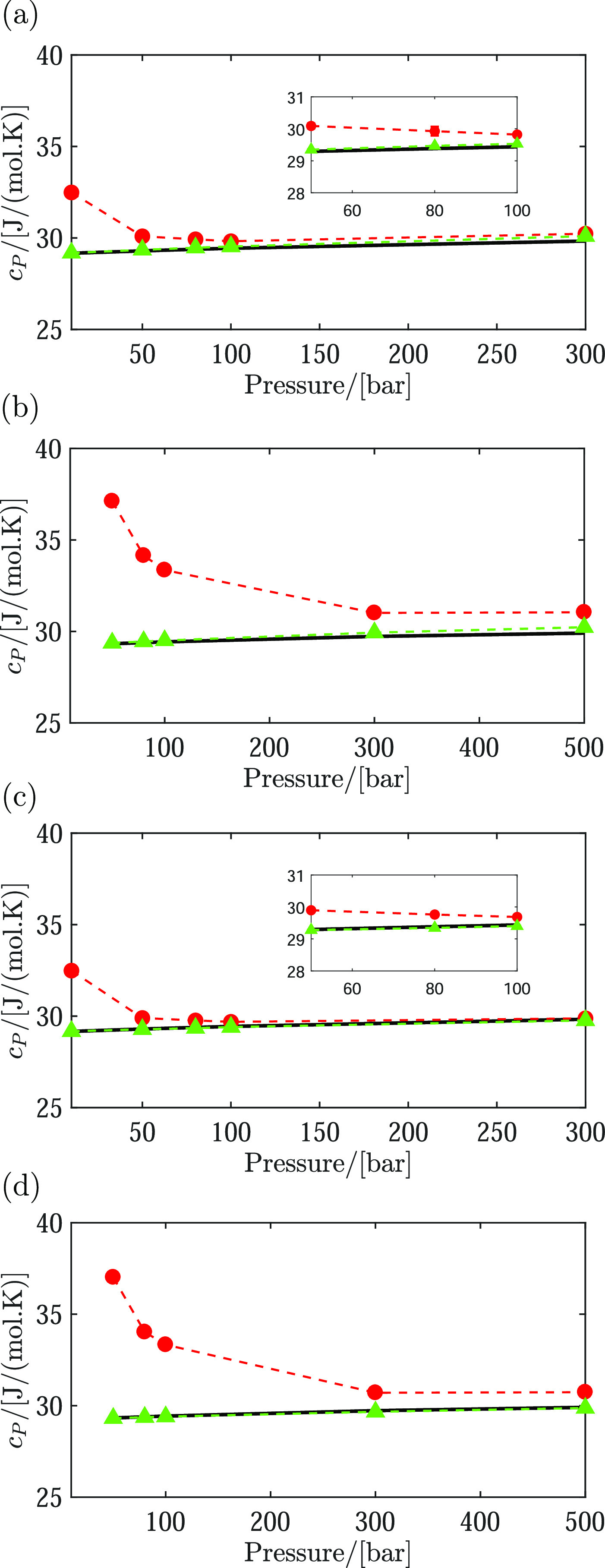
Heat capacities of hydrogen in the gas phase and hydrogen in the gas phase that is saturated with water. Triangles, pure hydrogen; circles, hydrogen–water mixtures; lines, empirical data for pure hydrogen from REFPROP.⁹² Heat capacities of mixtures computed using the TIP3P¹⁰⁰ and Marx⁹⁹ force fields are shown in subfigures (a) and (b) for T = 366 and 423 K, respectively. Heat capacities of mixtures computed using the TIP3P¹⁰⁰ and Vrabec¹⁰² force fields are shown in subfigures (c) and (d) for T = 366 and 423 K, respectively. The composition in the gas phase is obtained from VLE simulations of the water–hydrogen mixture at T = 423 and 366 K. Raw data obtained from molecular simulations (including the composition in the gas phase) are provided in Tables 4 and 5. Thermodynamic properties of pure hydrogen in the gas phase, obtained from REFPROP, are provided in Table S2 of the Supporting Information. Error bars are smaller than symbols.

Figure 5.

Joule–Thomson coefficients of hydrogen in the gas phase and hydrogen that is saturated with water. Triangles, pure hydrogen; circles, hydrogen–water mixtures; lines, empirical data for pure hydrogen obtained from REFPROP.⁹² Joule–Thomson coefficients of mixtures computed using the TIP3P¹⁰⁰ and Marx⁹⁹ force fields are shown in subfigures (a) and (b) for T = 366 and 423 K, respectively. Joule–Thomson coefficients of mixtures computed using the TIP3P¹⁰⁰ and Vrabec¹⁰² force fields are shown in subfigures (c) and (d) for T = 366 and 423 K, respectively. The composition in the gas phase is obtained from VLE simulations of the water–hydrogen mixture at T = 423 and 366 K. Raw data obtained from molecular simulations (including the composition in the gas phase) are provided in Tables 4 and 5. Thermodynamic properties of pure hydrogen in the gas phase, obtained from REFPROP, are provided in Table S2 of the Supporting Information. Error bars are smaller than symbols.

5.3. Chemical Potential of Ice, Water, and Hydrogen at the Melting Temperature

In Figure 6, the phase boundary diagram of water and ice Ih is shown. The corresponding data for this figure are obtained from experimental data.^91,92,108 The melting temperatures and pressures in Figure 6 are used for calculating chemical potentials of ice and water, from molecular simulation and empirical data. The IAPWS equation of state in REFPROP⁹¹ is used to calculate the chemical potential of ice and water along the melting line (T_m, P_m(T_m)). The results are shown in Figure 7, and the raw data are provided in Table 6. For hydrogen, excellent agreement is observed between the chemical potentials of the Marx force field and the chemical potentials obtained from REFPROP. The chemical potential computed with the TIP3P force field differs by a maximum of ca. 1 kJ/mol compared to the chemical potential obtained from the empirical equation of state of water.⁹¹ This difference does not cause significant deviation between the computed solubilities and the experimental solubilities of water in compressed hydrogen, as was shown in ref (38).

Figure 6.

Phase boundary diagram of water and ice Ih taken from experimental literature data.^91,92,108 The open circle indicates the solid–liquid–vapor triple point: P = 611.657 Pa and T = 273.16 K.⁹²

Figure 7.

Chemical potentials of pure hydrogen and water along the melting line of ice (T_m, P_m) computed from CFCMC simulations using the TIP3P¹⁰⁰ and Marx⁹⁹ force fields. Lines indicate the chemical potentials calculated from the empirical equation of states using REFPROP.⁹² Raw data are provided in Table 6. Error bars are smaller than symbols.

Table 6. Densities and Chemical Potentials of Pure Water and Pure Hydrogen along the Melting Line of Water^a.

pure water (TIP3P100)		CFCNPT		REFPROP92
Tm (K)	Pm (bar)	ρ (kg/m3)	(μ – μ0) (kJ/mol)	ρ (kg/m3)	(μ – μ0) (kJ/mol)
272.4	100	1010.6(4)	–34.4(1)	1004.8	–35.3491
270.79	300	1021.4(5)	–34.15(5)	1014.6	–35.0356
269.06	500	1032.1(4)	–33.80(3)	1024.1	–34.7292
266.73	750	1045.2(3)	–33.44(3)	1035.7	–34.3561
266.24	800	1047.1(5)	–33.40(6)	1038.0	–34.2829
264.21	1000	1056.9(4)	–33.12(5)	1046.9	–33.9943

pure hydrogen (Marx99)		CFCNPT		REFPROP92
Tm (K)	Pm (bar)	ρ (kg/m3)	(μ – μ0) (kJ/mol)	ρ (kg/m3)	(μ – μ0) (kJ/mol)
272.4	100	8.3906(4)	–13.304(5)	8.3665	–13.2887
270.79	300	22.5490(9)	–10.463(2)	22.317	–10.4301
269.06	500	33.860(3)	–8.944(4)	33.35	–8.89288
266.73	750	45.128(5)	–7.577(5)	44.315	–7.49641
266.24	800	47.094(5)	–7.338(5)	46.226	–7.25537
264.21	1000	54.203(4)	–6.466(8)	53.15	–6.36087

^aThe numbers in brackets indicate uncertainties in the last digit (95% confidence interval).

By changing the pressure, the equilibrium between ice and water shifts toward the most stable phase depending on the pressure. At different melting temperatures of ice, one can compute the chemical potentials of the most stable phase (liquid water or ice) as a function of pressure using eqs 12 and 14–16. This allows one to calculate the chemical potential of ice, based on empirical data without explicitly simulating the crystal structure of ice. The chemical potential of the most stable phase at each temperature can be calculated as a function of pressure using eqs 12 and 13. An example is provided in Figure 8 where the melting point of ice is at T = 266.73 K and P = 750 bar. It can be seen in Figure 8 that by increasing the pressure, the chemical potential of water would be lower than that of ice, which is the most stable phase for P > 750 bar. Decreasing the pressure would lead to having ice as the most stable phase.

Figure 8.

Chemical potentials of ice and water at T_m = 266.73 K as a function of pressure. Lines, crystalline ice; dashed lines, liquid phase. At this temperature, ice and water are in equilibrium at P_m = 750 bar. At P > P_m, the chemical potential of water is smaller than the chemical potential of ice, which indicates the most stable phase for that pressure range. For P < P_m, ice is the most stable phase. Raw data are provided in Table S3 of the Supporting Information, including different melting temperatures 264.21 K < T_m < 272.4 K. Equations 12 and 14–16 and the IAPWS equation of state for water⁹¹ were used to generate the data.

5.4. VLE of the Water–Hydrogen Mixtures at Freezing Temperature of Water

The VLE calculations of water–hydrogen mixtures are performed along the melting line of ice; see Figure 6. The corresponding melting temperatures and pressures for ice Ih are directly obtained from REFPROP.^91,92 One can obtain the same melting curve from ref (108). The melting temperatures selected in this work are between T = 272.4 and 264.21 K, which correspond to pressures between P = 100 and 1000 bar. It is crucial to consider the phase diagram of Figure 6 in precooling of the compressed hydrogen mixed with water (from the output of an EHC) and to calculate the amount of water dissolved in hydrogen at low temperatures. By performing independent simulations of the liquid phase (water) and the gas phase (hydrogen), the chemical potentials of water and hydrogen are computed along the melting line of ice. In Table 7, we provide an example to emphasize that the chemical potential of the solvent (water) is not affected by the chemical potential of the solute (hydrogen) at low concentrations. Due to the application of the EHC, the pressure range is limited to the range between P = 100 and 1000 bar. Using eqs 10 and 11, the VLEs of water–hydrogen mixtures were computed at the melting temperature of ice as a function of pressure. At each melting temperature, different pressures were considered for the VLE calculations (while remaining in the liquid water region). The results are shown in Figure 9. The raw data corresponding to the liquid phase are provided in Table 8, and the raw data corresponding to the gas phase are provided in Table 9. In Figure 9, only simulation results are provided, as to the best of our knowledge, no experimental VLE data of water and hydrogen, along the melting line of ice, are reported in the published literature. From simulations, the solubility of water is the highest at ca. 90 ppm (molar) at 272.4 K (and 100 bar) and the lowest at ca. 7 ppm (molar) at 264.21 K (and 1000 bar). Such low solubilities justify our choice of not using the Gibbs ensemble. The solubilities of hydrogen in the liquid phase vary between 0.01 and 0.001, corresponding to 272.4 and 264.21 K, respectively. It is well-known that to obtain solubilities in good agreement with experimental data, the accuracy of the chemical potentials of water and hydrogen obtained from the force fields is crucial. In the Supporting Information (Section S5), we provide an extended discussion on the importance of the chemical potentials (focusing on water) regarding the accuracy of solubility calculations for water–hydrogen systems. Additional VLE calculations of water–hydrogen mixtures were performed using the TIP3P and TIP4P/2005 force fields. For the purpose of this discussion, a modified force field based on the TIP4P/2005 force field is introduced in the Supporting Information, which improves the accuracy of solubility calculations simultaneously in the liquid and the gas phase.

Table 7. Computed Chemical Potentials of Water in Water–Hydrogen Mixtures Where the Mole Fraction of Hydrogen (x_H2) Is Close to Saturation^a.

T (K)	P (bar)	NH2	NH2O	xH2	(μ – μ0) (kJ/mol)
268	875	0	730	0	–33.2(2)
268	875	1	730	0.001	–33.3(2)
268	875	3	730	0.004	–33.3(2)
268	875	5	730	0.007	–33.3(2)
268	875	10	730	0.014	–33.1(2)
273	300	0	730	0	–34.1(2)
273	300	1	730	0.001	–34.1(2)
273	300	3	730	0.004	–34.1(2)
273	300	5	730	0.007	–34.1(2)
273	300	10	730	0.014	–34.1(2)
273	500	0	730	0	–33.8(2)
273	500	1	730	0.001	–33.7(2)
273	500	3	730	0.004	–33.7(2)
273	500	5	730	0.007	–33.7(2)
273	500	10	730	0.014	–33.7(3)
273	875	0	730	0	–33.1(2)
273	875	1	730	0.001	–33.1(2)
273	875	3	730	0.004	–33.1(3)
273	875	5	730	0.007	–33.2(2)
273	875	10	730	0.014	–33.1(3)
273	1000	0	730	0	–32.9(2)
273	1000	1	730	0.001	–32.9(2)
273	1000	3	730	0.004	–32.8(3)
273	1000	5	730	0.007	–32.9(2)
273	1000	10	730	0.014	–32.8(3)

^aThe mixture is defined using the TIP3P¹⁰⁰ and Marx⁹⁹ force fields.³⁸N_i is the number of molecules of component i. Numbers in brackets indicate uncertainties in the last digit (95% confidence interval).

Figure 9.

VLE of water–hydrogen at low temperatures as a function of pressure, obtained from eqs 10 and 11. (a) Mole fraction of water (y_H2O) in the gas phase. (b) Mole fraction of hydrogen (x_H2) in the liquid phase. For each temperature (T_m), the points on the dashed line correspond to the composition calculated at the melting pressure (P_m) of ice; see Table 6. For each value of T_m, solubility calculations are performed for pressures in the range between P_m and 1000 bar. The melting temperature and pressure were selected based on the values from the IAPWS equation of state.^91,92 Raw data, including the melting temperatures and pressures, are provided in Tables 8 and 9. Error bars are smaller than symbols.

Table 8. Densities of Water (ρ_H2O), Chemical Potentials of Water (μ_H2O – μ_H2O⁰), Excess Chemical Potentials of Hydrogen at Infinite Dilution in Liquid Water (μ_H2), and the Solubilities of Hydrogen in Liquid Water, Obtained from Simulations in the CFCNPT Ensemble^73,76,a.

T (K)	P (bar)	ρH2O (kg/m3)	(μH2O – μH2O0) (kJ/mol)	μH2ex (kJ/mol)	xH2/10–3
272.4*	100	1009.8(5)	–34.5(1)	9.18(3)	1.44(2)
272.4	300	1020.3(6)	–34.10(5)	9.58(5)	4.0(1)
272.4	500	1029.8(5)	–33.8(1)	10.01(4)	6.3(1)
272.4	750	1040.7(4)	–33.28(5)	10.46(3)	8.9(1)
272.4	1000	1051.5(5)	–32.89(4)	10.97(5)	11.2(3)
270.79*	300	1021.2(5)	–34.1(1)	9.56(4)	4.01(6)
270.79	500	1030.2(4)	–33.84(8)	9.93(4)	6.4(1)
270.79	750	1041.8(3)	–33.37(5)	10.45(4)	8.8(2)
270.79	1000	1052.5(3)	–32.85(7)	10.96(3)	11.0(2)
269.06*	500	1031.9(5)	–33.84(7)	9.90(4)	6.3(1)
269.06	750	1042.9(4)	–33.4(1)	10.38(4)	8.9(1)
269.06	1000	1053.6(1)	–32.96(6)	10.90(3)	11.0(1)
266.73*	750	1045.0(4)	–33.47(8)	10.35(6)	8.7(3)
266.73	1000	1055.1(6)	–33.1(1)	10.80(4)	11.2(2)
264.21*	1000	1056.9(3)	–33.15(6)	10.76(4)	11.0(2)

^aWater was simulated using the TIP3P force field, and a fractional molecule of hydrogen using the Marx force field⁹⁹ was added to the system. Stars indicate melting temperatures and the corresponding melting pressures for ice. x_H2 is the mole fraction of hydrogen in liquid water. Numbers in brackets indicate uncertainties in the last digit (95% confidence interval).

Table 9. Densities of Hydrogen (ρ_H2), Chemical Potentials of Hydrogen (μ_H2 – μ_H2⁰), Excess Chemical Potentials of Water at Infinite Dilution in Hydrogen (μ_H2O^ex), and the Solubilities of Water in Compressed Hydrogen, Obtained from Simulations in the CFCNPT Ensemble^73,76,a.

T (K)	P (bar)	ρH2 (kg/m3)	(μH2 – μH20) (kJ/mol)	μH2Oex (kJ/mol)	yH2O/10–6
272.4*	100	8.3776(6)	–13.31(1)	0.112(5)	87(5)
272.4	300	22.396(3)	–10.54(1)	0.394(9)	31(1)
272.4	500	33.475(2)	–9.10(1)	0.748(8)	20.8(5)
272.4	750	44.391(4)	–7.81(1)	1.24(1)	14.6(7)
272.4	1000	53.080(8)	–6.77(1)	1.746(7)	12.1(2)
270.79*	300	22.517(1)	–10.46(1)	0.400(7)	27.4(9)
270.79	500	33.635(3)	–9.02(1)	0.741(8)	18.7(8)
270.79	750	44.584(4)	–7.74(1)	1.228(9)	12.9(4)
270.79	1000	53.283(7)	–6.71(1)	1.73(1)	10.7(2)
269.06*	500	33.812(2)	–8.95(1)	0.73(1)	16.0(3)
269.06	750	44.788(2)	–7.67(1)	1.22(1)	11.7(4)
269.06	1000	53.505(3)	–6.65(1)	1.714(9)	9.5(5)
266.73*	750	45.072(5)	–7.58(1)	1.195(5)	10.1(3)
266.73	1000	53.808(3)	–6.56(1)	1.70(2)	8.1(3)
264.21*	1000	54.141(6)	–6.47(1)	1.671(5)	6.8(2)

^aHydrogen was defined using the Marx force field,⁹⁹ and a fractional molecule of water using the TIP3P force field¹⁰⁰ was added to the system. Stars indicate melting temperatures and the corresponding melting pressures for ice. y_H2O is the mole fraction of water in the gas phase. Numbers in brackets indicate uncertainties in the last digit (95% confidence interval).

Based on the solubility of hydrogen in liquid water along the melting line, one can calculate the freezing-point depression of water using eq 17. The results are shown in Table 10. The largest change in the freezing point of ice is around ΔT_F = 1 K, corresponding to 1.1% dissolved hydrogen in water at P = 1000 bar. At lower pressures, the freezing-point depression is less than 1 K.

Table 10. Freezing-Point Depression (ΔT_F) of Water as a Function of the Mole Fraction of Dissolved Hydrogen (x_H2)^57,a.

Tm (K)	Pm (bar)	xH2	ΔTF (K)
272.4	100	0.00144(2)	0.148(2)
270.79	300	0.00401(6)	0.407(6)
269.06	500	0.0063(1)	0.63(1)
266.73	750	0.0087(2)	0.86(2)
264.21	1000	0.011(2)	1.06(2)

^aT_m and P_m denote the freezing point of pure water. ΔT_F is obtained from eq 17. The mole fractions x_H2 are taken from Table 8. Numbers in brackets indicate uncertainty in the last digit.

6. Conclusions

In this work, we investigated the thermodynamic properties of hydrogen–water mixtures using molecular simulation. Using molecular-based modeling, we obtained important thermochemical properties of hydrogen–water mixtures, which are not readily available from experiments. Ensemble fluctuations were used to calculate thermodynamic derivatives from molecular simulation. The chemical potentials of water and ice were calculated along the melting line of ice. Different force fields for hydrogen (Cracknell,⁹⁷ Buch,¹⁰⁶ Hirschfelder,¹⁰⁷ Vrabec,¹⁰² and Marx⁹⁹) were used to calculate thermal expansivities, heat capacities, and the Joule–Thomson coefficients at high pressures. The heat capacities and thermal expansivities calculated using the Vrabec force field were in good agreement with experimental data. The results from other force fields agreed qualitatively well with the empirical results (e.g., following similar trends). No force field could very accurately calculate the Joule–Thomson coefficient of hydrogen; however, the qualitative behavior of the thermodynamic properties of hydrogen is correctly captured. The results obtained from the Vrabec and Marx force fields are closest to the experimental data. The TIP3P force field for water was used for simulating hydrogen–water mixtures and performing the VLE calculations, at temperatures and pressures corresponding to the melting line of ice Ih. From the commonly used rigid water models with point charges, the TIP3P force field is one of the best force fields for calculating the solubility calculations without using any binary interaction parameters. To examine the effect of the chemical potential on the VLE of water–hydrogen mixtures, a modified force field based on the TIP4P/2005 force field was introduced. Compared to the TIP4P/2005, the accuracy of the computed chemical potentials was significantly improved for the modified force field, which consequently led to some loss of accuracy for density predictions in the liquid phase. The computed solubilities of water in the gas phase using the modified TIP4P force field were similar to those obtained using the TIP3P force field. However, the modified TIP4P force field outperformed the TIP3P force field for the solubility of hydrogen in liquid water. Simulation results showed that thermodynamic properties of compressed hydrogen significantly change as the mole fraction of water in the gas phase is increased. For example, in sharp contrast to pure hydrogen, the Joule–Thomson coefficient of a saturated hydrogen–water mixture, containing 0.7% water (at T = 423.15 K and P = 100 bar), has a positive value, clearly showing that the effect of water cannot be neglected. At pressures above 700 bar, the solubility of water in hydrogen is low so that the behavior of the hydrogen–water mixture becomes very similar to the behavior of pure hydrogen. Experimental validation of the effect of water on thermodynamic properties of hydrogen would be very helpful and complementary to the simulations results. Unfortunately, to the best of our knowledge, such experimental data of the exact system at similar conditions are not available in the literature. The chemical potentials of water and ice along the melting of ice were obtained from molecular simulation and the IAPWS equation of state. For each melting temperature, the chemical potentials of water and ice were calculated as a function of pressure using experimental volumetric data. From the VLE of water–hydrogen, the compositions in the gas and liquid phase were obtained at low temperatures. The solubility calculations were performed in the pressure range between 100 and 1000 bar. The solubility of water in the gas phase is the highest at 100 bar (272.4 K), which is around 90 ppm (molar), and the solubility of hydrogen in the liquid phase is the highest at 1000 bar (264.21 K), which is around 1%. Based on the solubility data in the liquid phase, the freezing-point depression of water was calculated. The largest freezing-point depression is around 1.1 K corresponding to a pressure of 1000 bar and temperature of 264.21 K. For lower pressures, the freezing-point depression is very small. Our simulation results may have consequences for the energetics of a hydrogen refueling station using EHCs. This includes drying or precooling of the compressed hydrogen stream.

Supporting Information Available

The Supporting Information is available free of charge at https://pubs.acs.org/doi/10.1021/acs.jced.1c00020.

• Derivation of eqs 1 and 2; experimental data on the enthalpy difference between ice and water provided from the literature (Table S1); thermodynamic properties of pure hydrogen in the gas phase from REFPROP (fitted to experimental data) (Table S2); chemical potentials of ice and water as a function of temperature and pressure obtained from REFPROP (using the empirical equation of state for water) (Table S3); volumetric data of Ice Ih in Table S3 are obtained as a function of temperature using eqs 14–16;⁹³ discussion on the importance of the chemical potential of water to improve VLE calculations of water–hydrogen mixtures; parameters of the modified TIP4P force field (Table S5); VLE data of pure water and hydrogen–water mixtures using the modified TIP4P force field for water and the Marx force field for hydrogen (Tables S6 and S7) (PDF)

The authors declare the following competing financial interest(s): One of the authors (Julio C. Garcia-Navarro) was an employee of HyET Hydrogen BV, a Dutch company that is developing Electrochemical Hydrogen Compressors.

References

- Manoharan Y.; Hosseini S. E.; Butler B.; Alzhahrani H.; Senior B. T. F.; Ashuri T.; Krohn J. Hydrogen Fuel Cell Vehicles; Current Status and Future Prospect. Appl. Sci. 2019, 9, 2296 10.3390/app9112296. [DOI] [Google Scholar]
- Dincer I.; Acar C. Review and evaluation of hydrogen production methods for better sustainability. Int. J. Hydrogen Energy 2015, 40, 11094–11111. 10.1016/j.ijhydene.2014.12.035. [DOI] [Google Scholar]
- Jain I. Hydrogen the fuel for 21st century. Int. J. Hydrogen Energy 2009, 34, 7368–7378. 10.1016/j.ijhydene.2009.05.093. [DOI] [Google Scholar]
- Schorer L.; Schmitz S.; Weber A. Membrane based purification of hydrogen system (MEMPHYS). Int. J. Hydrogen Energy 2019, 44, 12708–12714. 10.1016/j.ijhydene.2019.01.108. [DOI] [Google Scholar]
- Wang D.; Liao B.; Zheng J.; Huang G.; Hua Z.; Gu C.; Xu P. Development of regulations, codes and standards on composite tanks for on-board gaseous hydrogen storage. Int. J. Hydrogen Energy 2019, 44, 22643–22653. 10.1016/j.ijhydene.2019.04.133. [DOI] [Google Scholar]
- Acar C.; Dincer I. Review and evaluation of hydrogen production options for better environment. J. Cleaner Prod. 2019, 218, 835–849. 10.1016/j.jclepro.2019.02.046. [DOI] [Google Scholar]
- Abe J.; Popoola A.; Ajenifuja E.; Popoola O. Hydrogen energy, economy and storage: Review and recommendation. Int. J. Hydrogen Energy 2019, 44, 15072–15086. 10.1016/j.ijhydene.2019.04.068. [DOI] [Google Scholar]
- Peschel A. Industrial Perspective on Hydrogen Purification, Compression, Storage, and Distribution. Fuel Cells 2020, 20, 385–393. 10.1002/fuce.201900235. [DOI] [Google Scholar]
- Sdanghi G.; Maranzana G.; Celzard A.; Fierro V. Review of the current technologies and performances of hydrogen compression for stationary and automotive applications. Renewable Sustainable Energy Rev. 2019, 102, 150–170. 10.1016/j.rser.2018.11.028. [DOI] [Google Scholar]
- Chen Y.; Zhang Z.; Tao F. Impacts of climate change and climate extremes on major crops productivity in China at a global warming of 1.5 and 2.0°C. Earth Syst. Dyn. 2018, 9, 543–562. 10.5194/esd-9-543-2018. [DOI] [Google Scholar]
- Dincer I. Environmental and sustainability aspects of hydrogen and fuel cell systems. Int. J. Energy Res. 2007, 31, 29–55. 10.1002/er.1226. [DOI] [Google Scholar]
- Dawood F.; Anda M.; Shafiullah G. M. Hydrogen production for energy: an overview. Int. J. Hydrogen Energy 2020, 45, 3847–3869. 10.1016/j.ijhydene.2019.12.059. [DOI] [Google Scholar]
- Casati C.; Longhi P.; Zanderighi L.; Bianchi F. Some fundamental aspects in electrochemical hydrogen purification/compression. J. Power Sources 2008, 180, 103–113. 10.1016/j.jpowsour.2008.01.096. [DOI] [Google Scholar]
- Muradov N.; Veziroğlu T. From hydrocarbon to hydrogen–carbon to hydrogen economy. Int. J. Hydrogen Energy 2005, 30, 225–237. 10.1016/j.ijhydene.2004.03.033. [DOI] [Google Scholar]
- Avendaño C.; Alejandro G.-V. Monte Carlo simulations of primitive models for ionic systems using the Wolf method. Mol. Phys. 2006, 104, 1475–1486. 10.1080/00268970600551155. [DOI] [Google Scholar]
- Kee B. L.; Curran D.; Zhu H.; Braun R. J.; DeCaluwe S. C.; Kee R. J.; Ricote S. Thermodynamic Insights for Electrochemical Hydrogen Compression with Proton-Conducting Membranes. Membranes 2019, 9, 77 10.3390/membranes9070077. [DOI] [PMC free article] [PubMed] [Google Scholar]
- Decourt B.; Lajoie B.; Debarre R.; Soupa O.. Hydrogen-Based Energy Conversion, More Than Storage: System Flexibility, 2014. http://www.4is-cnmi.com/feasability/doc-added-4-2014/SBC-Energy-Institute_Hydrogen-based-energy-conversion_Presentation.pdf (accessed Dec 1, 2020).
- Adolf J.; Balzer C. H.; Louis J.; Schabla U.; Fischedick M.; Arnold K.; Pastowski A.; Schüwer D.. Energy of the Future? Sustainable Mobility through Fuel Cells and H2; Shell Hydrogen Study; Shell Deutschland Oil, 2017; p 71. [Google Scholar]
- Murray L. J.; Dincǎ M.; Long J. R. Hydrogen storage in metal–organic frameworks. Chem. Soc. Rev. 2009, 38, 1294–1314. 10.1039/b802256a. [DOI] [PubMed] [Google Scholar]
- Najdi R. A.; Shaban T. G.; Mourad M. J.; Karaki S. H. In Hydrogen Production and Filling of Fuel Cell Cars, 3rd International Conference on Advances in Computational Tools for Engineering Applications (ACTEA), 2016; pp 43–48.
- Kuroki T.; Sakoda N.; Shinzato K.; Monde M.; Takata Y. Prediction of transient temperature of hydrogen flowing from pre-cooler of refueling station to inlet of vehicle tank. Int. J. Hydrogen Energy 2018, 43, 1846–1854. 10.1016/j.ijhydene.2017.11.033. [DOI] [Google Scholar]
- de Miguel N.; Acosta B.; Moretto P.; Ortiz Cebolla R. Influence of the gas injector configuration on the temperature evolution during refueling of on-board hydrogen tanks. Int. J. Hydrogen Energy 2016, 41, 19447–19454. 10.1016/j.ijhydene.2016.07.008. [DOI] [Google Scholar]
- de Miguel N.; Acosta B.; Baraldi D.; Melideo R.; Ortiz Cebolla R.; Moretto P. The role of initial tank temperature on refuelling of on-board hydrogen tanks. Int. J. Hydrogen Energy 2016, 41, 8606–8615. 10.1016/j.ijhydene.2016.03.158. [DOI] [Google Scholar]
- Hammerschlag R.; Mazza P. Questioning hydrogen. Energy Policy 2005, 33, 2039–2043. 10.1016/j.enpol.2004.04.010. [DOI] [Google Scholar]
- Das L. On-board hydrogen storage systems for automotive application. Int. J. Hydrogen Energy 1996, 21, 789–800. 10.1016/0360-3199(96)00006-7. [DOI] [Google Scholar]
- Bauer A.; Mayer T.; Semmel M.; Guerrero Morales M. A.; Wind J. Energetic evaluation of hydrogen refueling stations with liquid or gaseous stored hydrogen. Int. J. Hydrogen Energy 2019, 44, 6795–6812. 10.1016/j.ijhydene.2019.01.087. [DOI] [Google Scholar]
- Wical R. M.; Wical B.. Total Energy Independence for the United States: A Twelve-Year Plan, 1st ed.; iUniverse: Lincoln, England, 2007. [Google Scholar]
- Rohland B.; Eberle K.; Ströbel R.; Scholta J.; Garche J. Electrochemical hydrogen compressor. Electrochim. Acta. 1998, 43, 3841–3846. 10.1016/S0013-4686(98)00144-3. [DOI] [Google Scholar]
- Léon A.Hydrogen Technology: Mobile and Portable Applications, 1st ed.; Springer-Verlag: Berlin, Heidelberg, 2008. [Google Scholar]
- Bouwman P. Electrochemical Hydrogen Compression (EHC) solutions for hydrogen infrastructure. Fuel Cells Bull. 2014, 2014, 12–16. 10.1016/S1464-2859(14)70149-X. [DOI] [Google Scholar]
- HyET Hydrogen, Operating principle. https://hyethydrogen.com/technology/operating-principle/ (accessed Dec 1, 2020).
- Stolten D.Hydrogen and Fuel Cells: Fundamentals, Technologies and Applications, 1st ed.; Wiley-VCH Verlag GmbH & Co. KGaA: Weinheim, Germany, 2010. [Google Scholar]
- Nordio M.; Rizzi F.; Manzolini G.; Mulder M.; Raymakers L.; van Sint Annaland M.; Gallucci F. Experimental and modelling study of an electrochemical hydrogen compressor. Chem. Eng. J. 2019, 369, 432–442. 10.1016/j.cej.2019.03.106. [DOI] [Google Scholar]
- Ströbel R.; Oszcipok M.; Fasil M.; Rohland B.; Jörissen L.; Garche J. The compression of hydrogen in an electrochemical cell based on a PEM fuel cell design. J. Power Sources 2002, 105, 208–215. 10.1016/S0378-7753(01)00941-7. [DOI] [Google Scholar]
- Woodfield P. L.; Monde M.; Takano T. Heat Transfer Characteristics for Practical Hydrogen Pressure Vessels Being Filled at High Pressure. J. Therm. Sci. Technol. 2008, 3, 241–253. 10.1299/jtst.3.241. [DOI] [Google Scholar]
- Monde M.; Woodfield P.; Takano T.; Kosaka M. Estimation of temperature change in practical hydrogen pressure tanks being filled at high pressures of 35 and 70 MPa. Int. J. Hydrogen Energy 2012, 37, 5723–5734. 10.1016/j.ijhydene.2011.12.136. [DOI] [Google Scholar]; XII International Symposium on Polymer Electrolytes: New Materials for Application in Proton Exchange Membrane Fuel Cells.
- Fueling Protocols for Light Duty Gaseous Hydrogen Surface Vehicles; SAE International, 2020. https://www.sae.org/standards/content/j2601_202005/ (accessed Dec 1, 2020).
- Rahbari A.; Brenkman J.; Hens R.; Ramdin M.; van den Broeke L. J. P.; Schoon R.; Henkes R.; Moultos O. A.; Vlugt T. J. H. Solubility of water in hydrogen at high Pressures: a molecular simulation study. J. Chem. Eng. Data 2019, 64, 4103–4115. 10.1021/acs.jced.9b00513. [DOI] [Google Scholar]
- Kroenlein K. G.; Diky V.; Muzny C. D.; Chirico R. D.; Magee J. W.; Frenkel M. D.. ThermoLit: NIST Literature Report Builder for Thermophysical and Thermochemical Property Measurements; NIST, 2012. http://trc.nist.gov/thermolit (accessed Dec 1, 2020).
- Wiebe R.; Gaddy V. L. The solubility of hydrogen in water at 0, 50, 75 and 100° from 25 to 1000 atmospheres. J. Am. Chem. Soc. 1934, 56, 76–79. 10.1021/ja01316a022. [DOI] [Google Scholar]
- Meyer M.; Tebbe U.; Piiper J. Solubility of inert gases in dog blood and skeletal muscle. Pflügers Arch. 1980, 384, 131–134. 10.1007/BF00584428. [DOI] [PubMed] [Google Scholar]
- Gillespie P.; Wilson G.. Vapor–Liquid Equilibrium Data on Water-Substitute Gas Components: N2–H2O, H2–H2O, CO–H2O, H2–CO–H2O, and H2S–H2O, 1st ed.; Research Report; Gas Processors Association: Provo, Utah, 1980.
- Kling G.; Maurer G. The solubility of hydrogen in water and in 2-aminoethanol at temperatures between 323 K and 423 K and pressures up to 16 M Pa. J. Chem. Thermodyn. 1991, 23, 531–541. 10.1016/S0021-9614(05)80095-3. [DOI] [Google Scholar]
- Devaney W.; Berryman J. M.; Kao P.-L.; Eakin B.. High Temperature V–L–E Measurements for Substitute Gas Components, GPA Research Report; Gas Processors Association, 1978; pp 1–27.
- Jung J.Loslichkeit von Kohlenmonoxid und Wasserstoff in Wasser zwisen 0 C und 300 C. Ph.D. Thesis, RWTH: Aachen, 1962. [Google Scholar]
- Ipatev V.; Teodorovich V. Equilibrium compositions of vapor-gas mixtures over solutions. Zh. Obshch. Khim. 1934, 4, 395–399. [Google Scholar]
- Ugrozov V. V. Equilibrium compositions of vapor-gas mixtures over solutions. Russ. J. Phys. Chem. A 1996, 70, 1240–1241. [Google Scholar]
- Maslennikova V. Y.; Goryunova N.; Subbotina L.; Tsiklis D. The solubility of water in compressed hydrogen. Russ. J. Phys. Chem. B 1976, 50, 240–243. [Google Scholar]
- Bartlett E. P. The concentration of water vapor in compressed hydrogen, Nitrogen and a mixture of these gases in the presence of condensed water. J. Am. Chem. Soc. 1927, 49, 65–78. 10.1021/ja01400a010. [DOI] [Google Scholar]
- Dohrn R.; Brunner G. High-pressure fluid-phase equilibria: Experimental methods and systems investigated (1988-1993). Fluid Phase Equilib. 1995, 106, 213–282. 10.1016/0378-3812(95)02703-H. [DOI] [Google Scholar]
- Christov M.; Dohrn R. High-pressure fluid phase equilibria: Experimental methods and systems investigated (1994-1999). Fluid Phase Equilib. 2002, 202, 153–218. 10.1016/S0378-3812(02)00096-1. [DOI] [Google Scholar]
- Dohrn R.; Peper S.; Fonseca J. M. High-pressure fluid-phase equilibria: Experimental methods and systems investigated (2000-2004). Fluid Phase Equilib. 2010, 288, 1–54. 10.1016/j.fluid.2009.08.008. [DOI] [Google Scholar]
- Fonseca J. M.; Dohrn R.; Peper S. High-pressure fluid-phase equilibria: Experimental methods and systems investigated (2005–2008). Fluid Phase Equilib. 2011, 300, 1–69. 10.1016/j.fluid.2010.09.017. [DOI] [Google Scholar]
- Peper S.; Fonseca J. M.; Dohrn R. High-pressure fluid-phase equilibria: Trends, recent developments, and systems investigated (2009–2012). Fluid Phase Equilib. 2019, 484, 126–224. 10.1016/j.fluid.2018.10.007. [DOI] [Google Scholar]
- Frenkel D.; Smit B.. Understanding Molecular Simulation: From Algorithms to Applications, 2nd ed.; Academic Press: San Diego, California, 2002. [Google Scholar]
- Allen M. P.; Tildesley D. J.. Computer Simulation of Liquids, 2nd ed.; Oxford University Press: Oxford, United Kingdom, 2017. [Google Scholar]
- Sandler S. I.Chemical, Biochemical, and Engineering Thermodynamics; 4th ed.; John Wiley & Sons: Hoboken, NJ, 2006. [Google Scholar]
- Lagache M.; Ungerer P.; Boutin A.; Fuchs A. H. Prediction of thermodynamic derivative properties of fluids by Monte Carlo simulation. Phys. Chem. Chem. Phys. 2001, 3, 4333–4339. 10.1039/b104150a. [DOI] [Google Scholar]
- Moran M. J.; Shapiro H. N.. Fundamentals of Engineering Thermodynamics, 5th ed.; John Wiley & Sons: West Sussex, U.K., 2006. [Google Scholar]
- Schnell S. K.; Englebienne P.; Simon J.-M.; Krüger P.; Balaji S. P.; Kjelstrup S.; Bedeaux D.; Bardow A.; Vlugt T. J. H. How to apply the Kirkwood-Buff theory to individual species in salt solutions. Chem. Phys. Lett. 2013, 582, 154–157. 10.1016/j.cplett.2013.07.043. [DOI] [Google Scholar]
- Josephson T. R.; Singh R.; Minkara M. S.; Fetisov E. O.; Siepmann J. I. Partial molar properties from molecular simulation using multiple linear regression. Mol. Phys. 2019, 117, 3589–3602. 10.1080/00268976.2019.1648898. [DOI] [Google Scholar]
- Rahbari A.; Josephson T. R.; Sun Y.; Moultos O. A.; Dubbeldam D.; Siepmann J. I.; Vlugt T. J. H. Multiple Linear Regression and Thermodynamic Fluctuations are Equivalent for Computing Thermodynamic Derivatives from Molecular Simulation. Fluid Phase Equilib. 2020, 523, 112785 10.1016/j.fluid.2020.112785. [DOI] [Google Scholar]
- Jorgensen W. L. Optimized intermolecular potential functions for liquid alcohols. J. Phys. Chem. A 1986, 90, 1276–1284. 10.1021/j100398a015. [DOI] [Google Scholar]
- Becker T. M.; Wang M.; Kabra A.; Jamali S. H.; Ramdin M.; Dubbeldam D.; Infante Ferreira C. A.; Vlugt T. J. H. Absorption Refrigeration Cycles with Ammonia-Ionic Liquid Working Pairs Studied by Molecular Simulation. Ind. Eng. Chem. Res. 2018, 57, 5442–5452. 10.1021/acs.iecr.8b00442. [DOI] [PMC free article] [PubMed] [Google Scholar]
- Gutowski K. E.; Gurkan B.; Maginn E. J. Force field for the atomistic simulation of the properties of hydrazine, organic hydrazine derivatives, and energetic hydrazinium ionic liquids. Pure Appl. Chem. 2009, 81, 1799–1828. 10.1351/PAC-CON-08-09-24. [DOI] [Google Scholar]
- Reid R. C.; Prausnitz J. M.; Poling B. E.. The Properties of Gases and Liquids, 5th ed.; McGraw-Hill: New York, 2001. [Google Scholar]
- McQuarrie D. A.; Simon J. D.. Physical Chemistry: A Molecular Approach, 1st ed.; University Science Books: Sausalito, California, 1997. [Google Scholar]
- Johnson R. D., III, Ed. NIST Computational Chemistry Comparison and Benchmark Database, NIST Standard Reference Database Number 101, release 21; NIST, 2020. http://cccbdb.nist.gov/ (accessed Jan 7, 2021). [Google Scholar]
- Panagiotopoulos A. Z. Direct determination of phase coexistence properties of fluids by Monte Carlo simulation in a new ensemble. Mol. Phys. 1987, 61, 813–826. 10.1080/00268978700101491. [DOI] [Google Scholar]
- Panagiotopoulos A. Z.; Quirke N.; Stapleton M.; Tildesley D. Phase equilibria by simulation in the Gibbs ensemble: alternative derivation, generalization and application to mixture and membrane equilibria. Mol. Phys. 1988, 63, 527–545. 10.1080/00268978800100361. [DOI] [Google Scholar]
- Recht J.; Panagiotopoulos A. Z. Finite-size effects and approach to criticality in Gibbs ensemble simulations. Mol. Phys. 1993, 80, 843–852. 10.1080/00268979300102701. [DOI] [Google Scholar]
- Siepmann J. I.; McDonald I. R.; Frenkel D. Finite-size corrections to the chemical potential. J. Phys.: Condens. Matt 1992, 4, 679. 10.1088/0953-8984/4/3/009. [DOI] [Google Scholar]
- Rahbari A.; Hens R.; Ramdin M.; Moultos O. A.; Dubbeldam D.; Vlugt T. J. H. Recent advances in the continuous fractional component Monte Carlo methodology. Mol. Simul. 2020, 1–20. 10.1080/08927022.2020.1828585. [DOI] [Google Scholar]
- Shi W.; Maginn E. J. Continuous Fractional Component Monte Carlo: an adaptive biasing method for open system atomistic simulations. J. Chem. Theory Comput. 2007, 3, 1451–1463. 10.1021/ct7000039. [DOI] [PubMed] [Google Scholar]
- Shi W.; Maginn E. J. Improvement in molecule exchange efficiency in Gibbs ensemble Monte Carlo: development and implementation of the continuous fractional component move. J. Comput. Chem. 2008, 29, 2520–2530. 10.1002/jcc.20977. [DOI] [PubMed] [Google Scholar]
- Rahbari A.; Hens R.; Nikolaidis I. K.; Poursaeidesfahani A.; Ramdin M.; Economou I. G.; Moultos O. A.; Dubbeldam D.; Vlugt T. J. H. Computation of partial molar properties using Continuous Fractional Component Monte Carlo. Mol. Phys. 2018, 116, 3331–3344. 10.1080/00268976.2018.1451663. [DOI] [Google Scholar]
- Poursaeidesfahani A.; Torres-Knoop A.; Dubbeldam D.; Vlugt T. J. H. Direct free energy calculation in the Continuous Fractional Component Gibbs ensemble. J. Chem. Theory Comput. 2016, 12, 1481–1490. 10.1021/acs.jctc.5b01230. [DOI] [PubMed] [Google Scholar]
- Nezbeda I.; Kolafa J. A new version of the insertion particle method for determining the chemical Potential by Monte Carlo simulation. Mol. Simul. 1991, 5, 391–403. 10.1080/08927029108022424. [DOI] [Google Scholar]
- Smith J. M.; van Ness H. C.; Abbott M. M.. Introduction to Chemical Engineering Thermodynamics, 7th ed.; McGraw-Hill: New York, 2005. [Google Scholar]
- Pauling L. The Structure and Entropy of Ice and of Other Crystals with Some Randomness of Atomic Arrangement. J. Am. Chem. Soc. 1935, 57, 2680–2684. 10.1021/ja01315a102. [DOI] [Google Scholar]
- McBride C.; Vega C.; Sanz E.; MacDowell L. G.; Abascal J. L. F. The range of meta stability of ice-water melting for two simple models of water. Mol. Phys. 2005, 103, 1–5. 10.1080/00268970412331293820. [DOI] [Google Scholar]
- Buch V.; Sandler P.; Sadlej J. Simulations of H2O Solid, Liquid, and Clusters, with an Emphasis on Ferroelectric Ordering Transition in Hexagonal Ice. J. Phys. Chem. B 1998, 102, 8641–8653. 10.1021/jp980866f. [DOI] [Google Scholar]
- Parrinello M.; Rahman A. Crystal Structure and Pair Potentials: A Molecular-Dynamics Study. Phys. Rev. Lett. 1980, 45, 1196–1199. 10.1103/PhysRevLett.45.1196. [DOI] [Google Scholar]
- Espinosa J. R.; Vega C.; Sanz E. Ice-Water Interfacial Free Energy for the TIP4P, TIP4P/2005, TIP4P/Ice, and mW Models As Obtained from the Mold Integration Technique. J. Phys. Chem. C 2016, 120, 8068–8075. 10.1021/acs.jpcc.5b11221. [DOI] [Google Scholar]
- Frenkel D.; Ladd A. J. C. New Monte Carlo method to compute the free energy of arbitrary solids. Application to the fcc and hcp phases of hard spheres. J. Chem. Phys. 1984, 81, 3188–3193. 10.1063/1.448024. [DOI] [Google Scholar]
- Vega C.; Noya E. G. Revisiting the Frenkel-Ladd method to compute the free energy of solids: The Einstein molecule approach. J. Chem. Phys. 2007, 127, 154113 10.1063/1.2790426. [DOI] [PubMed] [Google Scholar]
- Vega C.; Sanz E.; Abascal J. L. F.; Noya E. G. Determination of phase diagrams via computer simulation: methodology and applications to water, electrolytes and proteins. J. Phys.: Condens. Matter. 2008, 20, 153101 10.1088/0953-8984/20/15/153101. [DOI] [Google Scholar]
- Vega C.; Abascal J. L. F.; Conde M. M.; Aragones J. L. What ice can teach us about water interactions: a critical comparison of the performance of different water models. Faraday Discuss. 2009, 141, 251–276. 10.1039/B805531A. [DOI] [PubMed] [Google Scholar]
- Wagner W.; Riethmann T.; Feistel R.; Harvey A. H. New Equations for the Sublimation Pressure and Melting Pressure of H2O Ice Ih. J. Phys. Chem. Ref. Data 2011, 40, 043103 10.1063/1.3657937. [DOI] [Google Scholar]
- Lemmon E. W.; Huber M. L.; McLinden M. O.. NIST Reference Fluid Thermodynamic and Transport Properties-REFPROP, version 7, NIST Standard Reference Database 23; NIST, 2002.
- Wagner W.; Pruß A. The IAPWS formulation 1995 for the thermodynamic properties of ordinary water substance for general and scientific use. J. Phys. Chem. Ref. Data 2002, 31, 387–535. 10.1063/1.1461829. [DOI] [Google Scholar]
- Lemmon E. W.; Huber M. L.; McLinden M. O.. NIST Reference Fluid Thermodynamic and Transport Properties-REFPROP, version 7, NIST Standard Reference Database 23; NIST, 2002. https://www.nist.gov/srd/refprop (accessed Jan 7, 2021).
- Marion G.; Jakubowski S. The compressibility of ice to 2.0 kbar. Cold Reg. Sci. Technol. 2004, 38, 211–218. 10.1016/j.coldregions.2003.10.008. [DOI] [Google Scholar]
- Petrenko V. F.; Whitworth R. W.. Physics of Ice, 1st ed.; Oxford University Press: U.K., 1999. [Google Scholar]
- Dickinson H. C.; Osborne N. S.. Specific Heat and Heat of Fusion of Ice, 1st ed., Bulletin of the Bureau of Standards 248; U.S. Department of Commerce, Bureau of Standards, 1916. [Google Scholar]
- Hens R.; Rahbari A.; Caro-Ortiz S.; Dawass N.; Erdős M.; Poursaeidesfahani A.; Salehi H. S.; Celebi A. T.; Ramdin M.; Moultos O. A.; Dubbeldam D.; Vlugt T. J. H. Brick-CFCMC: Open Source Software for Monte Carlo Simulations of Phase and Reaction Equilibria Using the Continuous Fractional Component Method. J. Chem. Inf. Model. 2020, 60, 2678–2682. 10.1021/acs.jcim.0c00334. [DOI] [PMC free article] [PubMed] [Google Scholar]
- Cracknell R. F. Molecular simulation of hydrogen adsorption in graphitic nanofibres. Phys. Chem. Chem. Phys. 2001, 3, 2091–2097. 10.1039/b100144m. [DOI] [Google Scholar]
- Deeg K. S.; Gutiérrez-Sevillano J. J.; Bueno-Pérez R.; Parra J. B.; Ania C. O.; Doblaré M.; Calero S. Insights on the Molecular Mechanisms of Hydrogen Adsorption in Zeolites. J. Phys. Chem. C 2013, 117, 14374–14380. 10.1021/jp4037233. [DOI] [Google Scholar]
- Marx D.; Nielaba P. Path-integral Monte Carlo techniques for rotational motion in two dimensions: quenched, annealed, and no-spin quantum-statistical averages. Phys. Rev. A 1992, 45, 8968–8971. 10.1103/PhysRevA.45.8968. [DOI] [PubMed] [Google Scholar]
- Jorgensen W. L.; Chandrasekhar J.; Madura J. D.; Impey R. W.; Klein M. L. Comparison of simple potential functions for simulating liquid water. J. Chem. Phys. 1983, 79, 926–935. 10.1063/1.445869. [DOI] [Google Scholar]
- Tsimpanogiannis I. N.; Moultos O. A.; Franco L. F. M.; Spera M. B. d. M.; Erdős M.; Economou I. G. Self-diffusion coefficient of bulk and confined water: a critical review of classical molecular simulation studies. Mol. Simul. 2019, 45, 425–453. 10.1080/08927022.2018.1511903. [DOI] [Google Scholar]
- Köster A.; Thol M.; Vrabec J. Molecular models for the hydrogen age: hydrogen, nitrogen, oxygen, argon, and water. J. Chem. Eng. Data 2018, 63, 305–320. 10.1021/acs.jced.7b00706. [DOI] [Google Scholar]
- Metropolis N.; Rosenbluth A. W.; Rosenbluth M. N.; Teller A. H.; Teller E. Equation of State Calculations by Fast Computing Machines. J. Chem. Phys. 1953, 21, 1087–1092. 10.1063/1.1699114. [DOI] [Google Scholar]
- Wang F.; Landau D. P. Efficient, multiple-range random walk algorithm to calculate the density of states. Phys. Rev. Lett. 2001, 86, 2050–2053. 10.1103/PhysRevLett.86.2050. [DOI] [PubMed] [Google Scholar]
- Rahbari A.; Hens R.; Dubbeldam D.; Vlugt T. J. H. Improving the accuracy of computing chemical potentials in CFCMC simulations. Mol. Phys. 2019, 117, 3493–3508. 10.1080/00268976.2019.1631497. [DOI] [Google Scholar]
- Buch V. Path integral simulations of mixed para-D2 and ortho-D2 clusters: the orientational effects. J. Chem. Phys. 1994, 100, 7610–7629. 10.1063/1.466854. [DOI] [Google Scholar]
- Hirschfelder C.; Curtiss F.; Bird R. B.. Molecular Theory of Gases and Liquids; Wiley: New York, 1954. [Google Scholar]
- IAPWS . Revised Release on the Pressure along the Melting and Sublimation Curves of Ordinary Water Substance; International Association for the Properties of Water and Steam, 2011. http://www.iapws.org/relguide/MeltSub2011.pdf (accessed Oct 1, 2020). [Google Scholar]
- Lemmon E. W.; Span R. Short fundamental equations of state for 20 industrial fluids. J. Chem. Eng. Data 2006, 51, 785–850. 10.1021/je050186n. [DOI] [Google Scholar]
Associated Data
This section collects any data citations, data availability statements, or supplementary materials included in this article.