

Abstract
Medical practitioners need to understand the critical features of ECG beats to diagnose and identify cardiovascular conditions accurately. This would be greatly facilitated by identifying the significant features of frequency components in temporal ECG wave-forms using computational methods. In this study, we have proposed a novel ECG beat classifier based on a customized VGG16-based Convolution Neural Network (CNN) that uses the time-frequency representation of temporal ECG, and a method to identify the contribution of interpretable ECG frequencies when classifying based on the SHapley Additive exPlanations (SHAP) values. We applied our model to the MIT-BIH arrhythmia dataset to classify the ECG beats and to characterise of the beats frequencies. This model was evaluated with two advanced time-frequency analysis methods. Our results indicated that for 2-4 classes our proposed model achieves a classification accuracy of 100% and for 5 classes it achieves a classification accuracy of 99.90%. We have also tested the proposed model using premature ventricular contraction beats from the American Heart Association (AHA) database and normal beats from Lobachevsky University Electrocardiography database (LUDB) and obtained a classification accuracy of 99.91% for the 5-classes case. In addition, SHAP value increased the interpretability of the ECG frequency features. Thus, this model could be applicable to the automation of the cardiovascular diagnosis system and could be used by clinicians.
Keywords: ECG, CNN, VGG16, ECG beats classification, SHAP value, ECG frequencies
Introduction
In recent years, the incidence of cardiovascular diseases (CVDs) have greatly increased worldwide, with CVDs now a leading cause of death in many countries [1]. Electrocardiograms (ECG) provide a non-invasive means of measuring the electrical activity of the heart and are commonly used to monitor and assess patient cardiac status. Unusual patterns of electrical activities in the heart occur with cardiac arrhythmia, and ECG can be used as part of the differential diagnosis process. Thus, for example, early detection of arrhythmia by analysis of ECG signals can greatly reduce the risk of death due to subsequent cardiac arrest.
Classification of normal and arrhythmia-associated ECG is an important goal to achieve better detection and proper identification of various CVDs. However, the small amplitude and duration of the ECG arrhythmia can make it challenging to classify using ECG data. Furthermore, variation in the normal ECG waveform of individual persons [2–5], the range of differences found in the patterns of ECG waveform associated with a particular CVD, and difficulties in distinguishing ECG waveform features seen in different patients with different CVDs make ECG rhythm classification challenging. The interpretation of the ECG and the management of the CVDs can be greatly improved with the assistance of computer-assisted diagnosis [6]. For this reason, there is great potential for deep learning-based computer-assisted tools to aid physicians in providing a better and more rapid diagnosis of arrhythmias. This can be achieved by developing such tools that can identify complex features in data, such as that seen in the beat characteristics of ECG signals.
In many studies [7–9], time-domain features of ECG signals, including RR intervals, QT segments, QRS complexes, and other morphological features have been identified by analyzing time-domain ECG signals. Using the peaks in ECG waveforms, an automatic monitoring system for the detection of normal, supraventricular ectopic beats and ventricular ectopic beats has been developed [8]. A previous study [10] used a linear prediction method, which detected ventricular premature contraction (VPC) with a sensitivity of 92%. Time-domain features were used to classify normal, supra-ventricular ectopic beats (SVEB) and ventricular ectopic beats (VEB) by applying a Hidden Markov Model (HMM) on various ECG segments [9]. Particle swarm optimization has been applied to ECG morphology and RR interval features to classify five types of arrhythmia beats, and this achieved an average accuracy of 93.27% [11]. Another study [12] addressed a six-class beats classification problem with an accuracy of 93.2% using the autoregressive model and generalized linear model classifier. Local fractal dimension has also been used to classify six types of ECG beats—atrial premature contraction (APC), left bundle branch block (LBBB), normal, paced beats, right bundle branch block (RBBB), and VPC—and classified with more than 97% sensitivity for normal, LBBB, RBBB, paced and VPC beats; more than 86% sensitivity for APC beats was seen [13]. Besides, Khazaee et al. [14] were able to classify five types of ECG beats (APC, LBBB, normal, RBBB, and VPC) with an accuracy of 93.97%. The ECG beats were classified with an accuracy of 96% using Hermite coefficients of ECG beats and neuro-fuzzy technique [15]. A Gaussian Mixture Model (GMM) has also been used to classify two types of abnormalities in the ECG and obtained accuracy greater than 94% [16]. In sum, a range of methods have been used to classify ECG beat data and have achieved good results, but with room for significant improvement.
The spectral domain of ECG signals offers another useful representation of the signal. Its parameters can give a distinctive signal representation which can be utilized for improving diagnostic accuracy. Some arrhythmia may cause time-domain changes that are subtle but greatly affect the ECG spectrum, which makes ECG beats more clearly distinct. A six-class classification was performed by Daamouche et al. using wavelet transform and particle swarm optimization technique to classify APC, LBBB, normal, paced beats, RBBB, and VPC, and this achieved an accuracy of 88.84% [17]. Another study [18] found that SVM (among a number of classifiers tested) performed best with an accuracy of 95.6% to classify normal and abnormal beats in ECG using features obtained by applying wavelet and PCA on ECG. Many studies have applied pre-processing techniques, feature extraction, and classification for ECG arrhythmia classification. In [19], Continuous Wavelet Transform (CWT) has been compared with DWT in ECG arrhythmia classification using multilayer percetron (MLP) and SVM machine learning model, it has been found that CWT based classifier improved the testing performance. A mixture of expert approached has been used to classify Normal, SVEB, VEB, and fusion beats and reported an accuracy of 94% [20]. The RR interval and morphological features were used in this classification. The block-based neural network on Hermite transform coefficients and RR interval features have also been used to classify five types of ECG beats and obtained 96.6% of accuracy [21]. Morphological wavelet transformation and time interval-based features were used to classify five ECG beats and obtained 95.16% accuracy [22]. Principal Component Analysis of normal, right bundle branch block, left bundle branch block, atrial premature contraction and ventricular premature contraction types ECG samples were performed in order to classify them and obtained an accuracy of 98.11% [23]. The principal components of bispectrum have been used to classify the same five types of ECG beats [24] and obtained an accuracy of 93.48%.
With the rise of deep learning techniques, a number of recent studies have used very deep networks for ECG beat classification, but many studies have not achieved 100% accuracy [20–31]. Acharya et al. [32] used a CNN algorithm to develop a method to detect myocardial infarction and obtained an average 95.22% classification accuracy. In another study, Acharya et al. [31] implemented a classifier based on a 9-layer deep CNN and classified five different types of heartbeats with an accuracy of 94.03%. Sannino and Pietro [27] presented a deep learning-based ECG beats classifier and obtained an overall accuracy of 99.83%. Isin et al. [33] used deep learning to classify ECG beats and obtained an accuracy of 92%. A deep learning-based automated diagnosis system for detecting congestive heart failure has also been developed using an 11-layer deep CNN model [34] and obtained 98.97% accuracy and sensitivity of 98.87%. However, the frequency components that are responsible for ECG beat variability were not reported in any of these studies. Identification of the frequency components could be crucial in better CVD management.
In this study, an accurate and optimal classification technique for ECG arrhythmia beat detection is proposed and a novel approach to identify differentiable frequency component features in ECG beats is also introduced. Our work offers two key contributions-
-
(i)
We proposed an adopted deep CNN, VGG16 [35], to classify 5 ECG beats using time-frequency representation of ECG signal. We evaluated the model with two advanced time-frequency representation techniques, CWT and Hilbert-Huang transform (HHT), to identify the best time-frequency representation of ECG beats for the CNN model.
-
(ii)
We harnessed explainable deep learning approach to identify crucial spectral features in ECG beats. We measured the SHapley Additive exPlanations (SHAP) value in the input image of the CNN model to find those pixel values in the scalogram which contribute most to the very high classification accuracy and map significant pixel values (wavelet coefficient) in the input image to corresponding frequency components in ECG beats.
The proposed adopted CNN with CWT scalogram achieved classification accuracies of 100% on MIT-BIH arrhythmia database for 2–4 classes and 99.90% for 5 classes. The American Heart Association (AHA) database and Lobachevsky University Electrocardiography database (LUDB) were also exploited for normal and ventricular contraction ECG beats, respectively, to test the proposed model and provided a classification accuracy of 99.91% for the 5-classes case. In addition, the SHAP-based identified spectral features in ECG show a considerably different band of frequencies in ECG beats that make them distinct to each other.
Materials and methods
The details of the datasets used in this study and the overall processing steps are summarized in Fig. 1. The ECG is segmented into pieces that contain three beats. Each ECG beat segment is fixed to 2.4 s long. Two signal-to-image conversion approaches were applied to produce input for classification model. The continuous wavelet transform was applied to each ECG segment to obtain the scalogram which represents the wavelet coefficient matrix of that segment. This scalogram was used as the input to the proposed classification model. Hilbert-huang tranform (HHT) was also applied to produce the model input in order to evaluate signal-to-image conversion approaches for the proposed classifier. An adopted deep learning model was trained using both the scalogram and HHT spectrum separately. The convolutional parts of the model extracted the feature map and classified the ECG segment into specific categories. Finally, we calculated the SHAP value to explain the significant frequency components in ECG beats. The classification results and SHAP-based significant components information is provided to the doctor/clinicians as report for patient treatment and management.
Fig. 1.

The schematic diagram of the proposed method
Database
In this study, the MIT-BIH arrhythmia database is used for the classification of the ECG arrhythmia and the detection of characteristic frequencies in ECG beats. The database consists of 48 records of half-hour. Two channels have been used to record the ECG. The ECG signals were obtained from 47 subjects between 1975 and 1979 at the BIH Arrhythmia Laboratory [36]. The first lead is modified lead II (MLII) that is used for 45 recordings, and for the remaining recording, modified lead V5 is used. The pericardial lead (V1 for 40 of them, V2, V4, or V5 for the others) is used as the second lead. In this study, only the MLII lead has been used. We have selected five different ECG beats, namely, normal (N), left bundle branch block (L), right bundle branch block (R), paced beat (PB), and premature ventricular contractions (V) for classification and analysis.
Data prepossessing
The MIT-BIH arrhythmia dataset is band-pass filtered at 0.1100 Hz and sampled at 360 Hz [37]. The annotation file in the MIT-BIH database contains information about the rhythms type and each individual heartbeat occurrence sample at the major local maxima. Thirty six files were chosen from the MIT-BIH arrhythmia database which contains the beats to be studied.
Beat segmentation
In the segmentation of the beat, we used the annotation files as a reference. For beat segmentation, first, the local maxima of each heartbeat (R peaks for most cases) are extracted from the annotation files, and a fixed number of samples are specified before and after each R peak. The box plot shown in Fig. 2a depicts distribution of duration of ECG segments in seconds that contains three consecutive beats obtained from all the files that contain all the beats to be analysed. Since we want to include at least one beat before and one beat after R peaks of the analyzed beat for 2-dimensional time-frequency representation, we choose a total of 865 sample points ( 1.2 s before and 1.2 s after R peaks). The choice of the window length of samples around the beats chosen is 2.4 s so that it contains approximately three cycles of cardiac activity. Total 8691 N beats segments, 8059 L beat segments, 7235 R beat segments, 7012 PB beat segments, and 7003 V beat segments were collected from 36 MIT-BIH files which includes files names 100, 101, 102, 103, 104, 105, 106, 107, 108, 109, 111, 114, 116, 118, 119, 124, 200, 201, 202, 203, 205, 207, 208, 210, 212, 213, 214, 215, 217, 219, 221, 223, 228, 231, 232, and 233. All of the records came from total 35 subjects; 34 records from 34 individual subjects and two records (201 and 202) from a single subject.
Fig. 2.
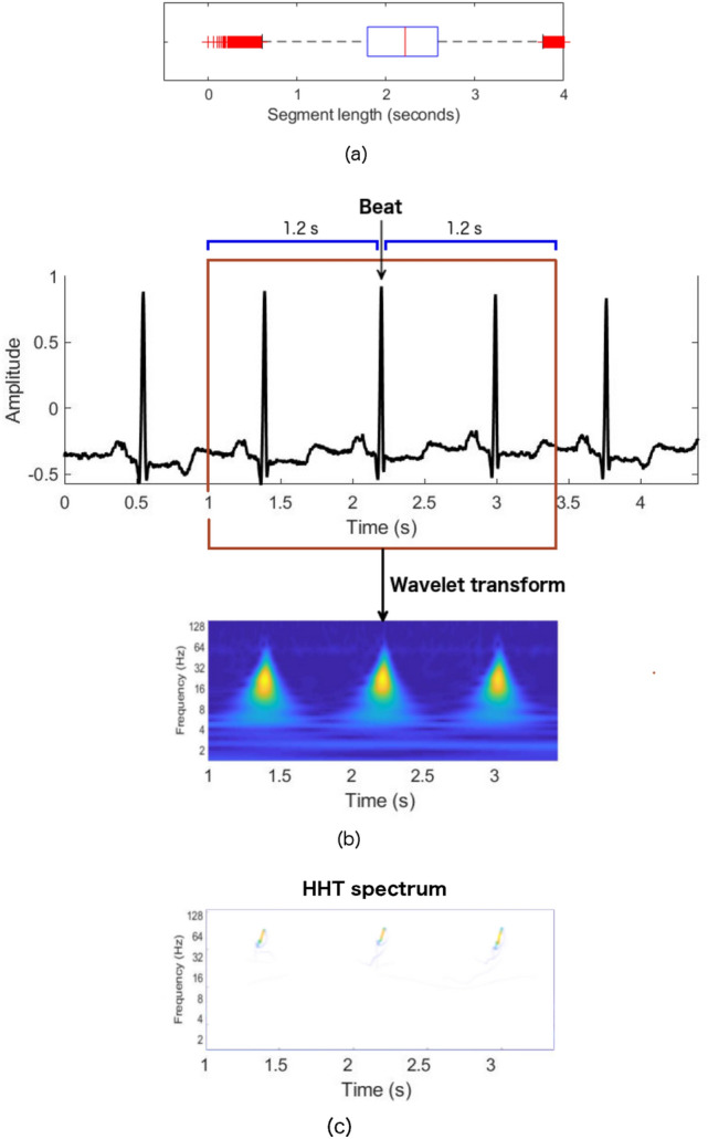
a Box plot of the distribution of the duration of ECG segments that contains three consecutive beats. b ECG beats segmentation and its scalogram, c Hilbert-Huang spectrum
From the MIT BIH database, a total of 38000 beat segments were considered for analysis. Figure 3 shows the stacked bar plots of the number of beat segments of each type obtained from 36 files. Four different datasets were prepared using these beat segments. The first dataset (DB I) contains ECG beat segments from two categories: N and L. The second dataset (DB II) contains ECG beat segments from three categories: N, L, and R. The third dataset (DB III) contains ECG beat segments for the N, L, R, and PB ECG beat classes. The fourth dataset (DB IV) consists of ECG beat segments corresponding to five different categories: N, L, R, PB, and V. The distribution of the number of beat segments from each of the classes and the datasets are given in Table 1. In this study, the entire dataset (38000 beat segments) was randomly sub-sampled into training, validation, and testing. In total 8291, 7659, 6835, 6612, and 6603 samples for N, L, R, PB, and V, respectively, beat segments were used for training the model. The remaining beat segments were used for testing and validation of the model. From the remaining beat segments 200 beat segments of each type are randomly selected to create a test set. There are a total of 1000 beat segments for validation and 1000 beat segments for testing of the model.
Fig. 3.

Stacked bar plot of the number of beat segments of each types collected from 36 files (35 subjects). Total 38000 beat segments are collected for five beat types
Table 1.
The datasets, class names, distribution of the number of beat segments in each dataset. The N, L, R, PB, and V beats are taken from 36 MIT-BIH files
| Dataset | Beat classes | ||||
|---|---|---|---|---|---|
| N | L | R | PB | V | |
| DB I | 8691 | 8059 | N/A | N/A | N/A |
| DB II | 8691 | 8059 | 7235 | N/A | N/A |
| DB III | 8691 | 8059 | 7235 | 7012 | N/A |
| DB IV | 8691 | 8059 | 7235 | 7012 | 7003 |
Continuous wavelet transform (CWT) for feature image preparation
Here, we present the feature image of ECG beats that we used for classification. The time-frequency representation of the ECG signal is produced using CWT for the classification.
The continuous wavelet transform has emerged as one of the most powerful tools for the high-resolution decomposition in the time-frequency plane of a signal. CWT is also a widely used method for the time-frequency analysis of a signal. It overcomes the limitations of Fourier transformation (FT), where no time information is available in the frequency domain representation. Wavelet transform is particularly crucial due to its capacity to elucidate simultaneously local spectral and temporal information from a non-stationary signal. The wavelet transforms isolates the signal component to produce a time-frequency representation of the signal by using a variable-length window, and this is more accurate than the traditional short-time Fourier transform (STFT) where a sliding time window of fixed length is used. Wavelet transform is a suitable choice for non-stationary signals, like ECG, and can be an alternative to the widely-used STFT. The lower frequency component in long duration signal and higher frequency component in the shorter duration signal are also captured simultaneously because of the flexible temporal-spectral aspect of the transform, which enables a local-dependent spectral analysis of individual signal components. We can decompose the ECG signal onto a set of basis functions, which are termed wavelets. All the basic functions are derived from a prototype wavelet by dilations and scaling, and translations. In fact, in wavelet transform, the frequency is considered to be an alternative to scale, leading to a time-frequency representation of the time-domain signal.
The prototype wavelet, used in this study to take the wavelet transform of the ECG signal, is defined as
| 1 |
Then the CWT of a signal x(t) is defined as:
| 2 |
where a is the scaling parameter and b is the translation parameter.
Using Morlet wavelet base in obtaining wavelet coefficient matrix by continuous wavelet transform showed promising result in a study [38] to classify ECG arrhythmia using deep learning model. In this study, we have determined to use the Morlet wavelet basis function which is defined as:
| 3 |
We can obtain the characteristic frequency of the wavelet from the wavelet scale a. The spectral components f’s are inversely proportional to the scale a’s, i.e. . The frequency associated with a wavelet of arbitrary scale a is given by
| 4 |
where the constant is the characteristic frequency of the mother wavelet at and , is the sampling frequency of x(t), and f is the frequency of the wavelet at arbitrary scale a.
After calculating the characteristic frequency, a time-frequency representation of the signal is obtained. The image form of the CWT time-frequency representation of the signal is called a scalogram. The scalograms were generated by performing CWT to all the segmented ECG beats. The segmented ECG beat and its corresponding scalogram are shown in Fig. 2b. The duration of the segmented ECG is 2.4 s (1 s to 3.4 s); the x-axes of the scalogram corresponds to the same time duration as the segmented ECG. The x and y axes of the scalogram represent time and frequency information of ECG, respectively, where the color represents the magnitude of the frequency components at that time point. The dark color represents the lower, and bright color represents the higher magnitude of the frequency.
Hilbert-Huang transform for feature image preparation
We evaluated the classifier used in this study with the Hilber-Huang transform spectrum. The Hilbert-Huang transform (HHT) [39] has widely been used for non-stationary signal processing as a powerful time-frequency technique. The HHT performs a data adaptive decomposition to decompose the signals into a set of nearly orthogonal components. The Hilbert-Huang spectrum is obtained by producing a time-frequency distribution of the signals.
HHT functions in two steps, namely, empirical mode decomposition (EMD) and Hilbert transform. The EMD decomposes a signal into a series of oscillatory modes called intrinsic mode function (IMF), and a residue. After applying EMD to a x(t), we have a collection of n number of IMFs denoted as and residue as-
| 5 |
After obtaining all the IMFs, we apply Hilbert transform to each IMF. This can be done by performing a convolution operation of the signal x(t) with the function , i.e.,
| 6 |
Now the analytic signal z(t) of x(t) can be defined by combining x(t) and H(t) as
| 7 |
where
| 8 |
Here a(t) and are the instantaneous amplitude and the instantaneous phase of x(t), respectively.
According to the property of Hilbert transform if x(t) is monocomponent, then the instantaneous frequency of x(t) can be defined as-
| 9 |
The IMFs of x(t) generated applying EMD are monocomponent. By calculating the instantaneous frequency and amplitude of each IMF, x(t) can be expressed as follows
| 10 |
The signal x(t) can be represented by a three dimensional time-frequency plane using Eq. 10. This time-frequency representation of the signal is called the Hilbert-Huang spectrum.
The Hilbert-Huang spectrum of each of the segmented ECG signals is obtained to evaluate the performance of the beat classification model.
Convolutional neural network (CNN)
The CNNs are one of the most advanced forms of deep artificial neural network architectures specifically designed for 3D image inputs. A CNN mainly consists of input layers, convolutional layers, activation layer, pooling layer, dense layer, and softmax (output) layer. There may be many hidden layers in the CNN, because of that, it is categorized as deep learning.
The input layer is associated with the input of the neural network. The input layer is a tensor of the dimensions of the input image. One of the critical layers is the convolutional layer, which comprises with a set of kernels (filters). The convolutional layers carry out the convolutional operation taking data from the previous layer. The convolutional operation is implemented by an inner product between the kernel and the image section that it covers. The computed convolutional operation produces a feature map, which is the response of the filter at every pixel location in the image. There are many such kernels in the convolutional layer, thus producing many 2D feature maps. After the completion of the convolution operations using the kernels, a stack of feature maps is produced, which are fed into the next layer. The activation function works in the activation layer. Rectified Linear Unit (ReLu) is the activation function usually used in the convolutional layer. The operation of this function is straightforward, it only remains a positive value the same but changes the negative input value to zero.
The pooling layer reduces the size of the feature map by downsampling the extracted features in the convolution layer. Two types of pooling layers, max pooling and average pooling, are widely used in many CNNs. The feature maps are segmented into non-overlapping squares in the pooling layer. In the max-pooling layer, the maximum values of the segments are taken, whereas, in the average pooling layer, the average values from the segments are computed, thus producing the reduced dimensional feature matrices. After the last process of pooling in the convolutional layers, the image is flattened and fed into a dense layer in the feed-forward neural network. The dense (fully connected) layers are the artificial neural networks that take input from the previous convolutional layers of the networks. The activation function in this layer is also ReLu, except for the last layer activated with the softmax function. The dense layer combines all local features into global features to obtain the probability of each of the desired classes. The softmax activated the top layer of the model can decide on the image class. This layer is used to learn non-linear combinations in high-level feature coming from the previous dense layers.
Once the model of CNN is completed, it is ready to update the network weights using the training dataset. Since CNN has many parameters that need to be updated, it takes a considerable time to train, and graphical processing units (GPUs) are required for faster training. To avoid computational complexity, it is recommended to use a pre-trained model that showed a good performance on a related task. We can do this by transfer learning. The classifier parts of the model are customized in order to have better performance. Fine-tuning the model by initializing the network weights with transfer learning provides a better model performance than the model being used without fine-tuning.
The customized classification model consists of VGG16 architecture used in this study is shown in Fig. 4. The VGG16 is a convolutional neural network (CNN) consists of 16 layers to classify a 224 x 224 input image. The customized classifier layers possess five fully-connected layers, the last of which is a softmax layer that provides the probability of each input to belong to a beat class. The first FC layer in the dense layers of the adopted CNN is consisted of 256 relu activated nodes. The second FC layer is consisted of 512 relu activeted nodes. The third FC layer is a dropout layer with a 50% dropout. The last layer provides the class probability of each input sample. The weights of the VGG16 parts of the model are initialized using transfer learning and the rest of the model, the dense layers, are randomly initialized. The whole model is now fine-tuned using the training datasets to get the optimized weights of the networks in order to obtain desired performance.
Fig. 4.

The proposed classification model consists of VGG16 and customized classifier layers
The input of the VGG16 is the segmented ECG beats images. In the first convolutional layer, 64 kernels were used with a very small receptive field (3 × 3 filter size) for feature extraction from the input images. The convolution stride size is 1 pixel. The input image size of the VGG16 is 224 × 224 RGB. In order to preserve the spatial resolution after convolution, the spatial padding of the convolution input layer is fixed to 1 pixel for 3 × 3 filter size. Max-pooling operation functions over a 2 × 2 pixel window, with a 2-pixel stride size.
Performance metrics
The performance metrics of sensitivity (Se), Specificity (Sp), Area Under the ROC curve (ROC), and Accuracy (Acc) are used to evaluate the ECG beats classifier. Sensitivity is a measure of the proportion of true positive beats to the total of true positive (TP) and false negative (FN) beats. Mathematically, sensitivity (Se) can be defined as:
| 11 |
Specificity (Sp) is defined as the proportion of true negative (TN) beats and to total of true negative (TN) and false positive (FP) beats. Mathematically, specificity can be defined as:
| 12 |
The accuracy (Acc) is defined as:
| 13 |
The ROC curve is drawn using sensitivity and specificity and the model performance is determined using the Area under the ROC curve (AUC). Here we use the micro averaging metric for AUC calculation.
Higher values of Se, Sp, Acc, and AUC indicate a better model.
Gradient based method for explaining important features
The black-box nature of CNN makes it difficult to explain the significance of input features that lead to high classification performance. A model interpretation method was used to reveal the importance of the features based on the model prediction results. The main objective of the interpretation process is to measure the SHAP (SHapley Additive exPlanations) [40] of the input features. Consider a set of N features Q and a function determines the outcome of the model when feature subset is used. The SHAP values are determined by quantifying the total contribution of each feature to the result of the model when all features are considered. For a given feature j, Shapley value can be computed as-
| 14 |
where is the contribution of feature j to the model prediction and it can be interpreted as its’ average marginal contribution.
Model interpretation approaches that are commonly used for CNN can be divided into two major groups. The first method is the gradient-based approach where the gradient is calculated using backpropagation, and the contribution score of input features for the target class is measured from this gradient. The second is the additive attribution method, which allows a description of the complex model by constructing a simpler model by alternative means. A gradient-based approach has been used in this study, discussed below.
The SHAP value for the feature in the input layer of the VGG16 model was calculated using the expected gradients [41]. Expected gradients are an improved version of integrated gradients [42], which use a small selection of hyperparameters. Integrated gradient attempts to explain the difference between the current prediction of the model and the model prediction with a given baseline input. In order to represent any uninformative reference information, the baseline input is used. Sometimes, the baseline input choice is made arbitrarily. However, the expected gradients model avoids using an arbitrary baseline and chooses baseline by integrating the value of the feature over a dataset.
The integrated gradient value of a feature i for a given model h is defined as:
| 15 |
where t and are the target and baseline inputs, respectively, and
| 16 |
In order to avoid specifying , the expected gradient (ExG) value for the feature i is defined as:
| 17 |
where D is the underlying data distribution. Since integrating over the training distribution is difficult, the integral is defined in expectation:
| 18 |
where
| 19 |
Finally, the expected based formula takes the sample t from the training dataset and from U(0, 1). It computes the expected value for each t and calculate the average overall drawn samples.
Results
The model training platform consisted of a gaming laptop computer with Intel(R) Core (TM) i7-7700HQ (2.80 GHz, 2808 Mhz, 4 Cores and 8 Logical processors) CPU, and a GPU of NVIDIA GeForce GTX 1060 6GB GPU and 16 GB of memory, running on a Windows 10 64-bit system. The experiments were conducted using the Matlab and Python programming languages. The software tools used in this study included Python 3.5, CUDA 9.0, and Matlab R2018a. The classification and explanation experiments were implemented using the Keras [43] library.
Accuracy and loss plots at each epoch of model training and validation with training and validation scalograms, respectively, are shown in Fig. 5. For the first few epochs of training and validation, the accuracy is slightly lower than that of the next epochs. The blue and red curves reach a final accuracy of 100% after 21 epochs and 3 epochs, respectively, and show the benefits of using the VGG16 CNN based classifier in the classification.
Fig. 5.

Classification accuracy and loss while training and validating the classifier using scalograms. The blue, red, green, and purple curves show training accuracy, validation accuracy, training loss, and validation loss, respectively. (Color figure online)
Table 2 shows test accuracy for all the test datasets using VGG16 without any modification and transfer learning, VGG16 without any modification and fine-tuning, modified VGG16 and fine-tuning. In order to compare the CWT scalogram with the HHT spectrum in deep learning based arrhythmia detection, the test results were obtained for both imaging techniques. The original VGG16 with transfer learning only and HHT spectrum showed a classification accuracy of 95.75%, 89%, 81.38%, and 72.70% for DB I, DB II, DB III, and DB IV, respectively. The accuracy trends to reduce with the increase in the number of test classes in the data sets. The VGG16 with original classifier and CWT scalogram presented a sensitivity of 100%, specificity of 100%, accuracy of 100% and AUC of 100% with test data of DB I and DB II. However, with test data of DB III and DB IV, which contains 4 and 5 classes of beats, respectively, the original classifier with scalogram shows relatively less accuracy than with the test data of DB I and DB II. For DB III, a sensitivity of 96.63%, specificity of 98.88%, accuracy of 96.63% and AUC of 97.75% was achieved. For DB IV, it presented a sensitivity of 95.10%, specificity of 98.78%, accuracy of 95.10% and AUC of 96.94%. For original VGG16 and transfer learning CWT scalogram showed better performance than the HHT spectrum.
Table 2.
Experimental results obtained with test dataset using VGG16 with original classifier layers in [35] and transfer learning, fine-tuned VGG16 with original classifier layers, and fine-tuned VGG16 with proposed customized classifier layers
| VGG16 model and training method | Imaging method | Dataset | Acc (%) | Se (%) | Sp (%) | AUC (%) |
|---|---|---|---|---|---|---|
| Transfer learning only | HHT | Dataset I | 95.75 | 95.75 | 95.75 | 95.75 |
| Dataset II | 89 | 89 | 94.5 | 91.75 | ||
| Dataset III | 81.38 | 81.38 | 93.79 | 87.58 | ||
| Dataset IV | 72.70 | 72.70 | 93.17 | 82.93 | ||
| CWT | Dataset I | 100 | 100 | 100 | 100 | |
| Dataset II | 100 | 100 | 100 | 100 | ||
| Dataset III | 96.63 | 96.63 | 98.88 | 97.75 | ||
| Dataset IV | 95.10 | 95.10 | 98.78 | 96.94 | ||
| Fine-tuning with original FC layers | HHT | Dataset I | 99.25 | 99.25 | 99.25 | 99.3 |
| Dataset II | 97.83 | 97.83 | 98.92 | 98.38 | ||
| Dataset III | 96.25 | 96.25 | 98.75 | 97.5 | ||
| Dataset IV | 95.70 | 95.70 | 98.93 | 97.3 | ||
| CWT | Dataset I | 100 | 100 | 100 | 100 | |
| Dataset II | 100 | 100 | 100 | 100 | ||
| Dataset III | 99.50 | 99.50 | 99.83 | 99.67 | ||
| Dataset IV | 98 | 98 | 99.5 | 98.75 | ||
| Fine-tuning with proposed customized FC layers | HHT | Dataset I | 100 | 100 | 100 | 100 |
| Dataset II | 97.83 | 97.83 | 98.92 | 98.38 | ||
| Dataset III | 97 | 97 | 99 | 98 | ||
| Dataset IV | 96.70 | 96.70 | 99.17 | 97 | ||
| CWT | Dataset I | 100 | 100 | 100 | 100 | |
| Dataset II | 100 | 100 | 100 | 100 | ||
| Dataset III | 100 | 100 | 100 | 100 | ||
| Dataset IV | 99.90 | 99.90 | 99.98 | 99.94 |
Bold texts indicate significant results
A classifier model with fine-tuned VGG16 with original FC layers was also evaluated for both scalogram and HHT spectrum. In this case, the CWT scalogram showed better performance than the HHT spectrum, details in Table 2.
In order to analyze the performance of the proposed classifier (fine-tuned VGG16 with customized FC layers), the test results were obtained for all the datasets with the CWT scalogram and HHT spectrum. For all the four test datasets, the classifier shows very high performance with the CWT scalogram. The sensitivity and specificity values tested for DB I, DB II, and DB III datasets are 100% and the accuracy is very high, 100%, in all the three cases. The classifier has an AUC of 100% for the DB I, DB II, and DB III datasets. For DB IV, the customized fine-tuned model with the CWT scalogram showed an accuracy of 99.90% with an AUC of 99.94%. The same model is also evaluated for the HHT spectrum. For all the cases, the CWT scalogram overperformed the HHT spectrum. It can also be observed that the proposed model is basically better than the model with the original VGG16 according to the accuracy of the classification. The ROC curves of the proposed model tested on the test datasets consisted of the CWT scalogram are shown in Fig. 6. The AUC for prediction of classes (N, L) from dataset I, classes (N, L, R) from dataset II, and classes (N, L, R, PB) from dataset III was 100%, and for classes (N, L, R, PB, V) from dataset IV was 99.9%. The confusion matrix is also used to show the classification results of the model. Figure 7 gives the confusion matrix showing the classification performance of the proposed classifier using test datasets of scalograms. The test dataset consists of 200 ECG beat segments for each type. The results indicate that the model can successfully separate the ECG beats.
Fig. 6.

Receiver operating characteristic (ROC) curves of customized VGG16 based CNN model tested on the various test ECG arrhythmia datasets. The ROC curves show the performance of the classifier for classifying ECG beats. The model presents the micro averaged AUC of 1.00 for the DB I, DB II, DB III test data and 0.999 for the DB IV test set
Fig. 7.
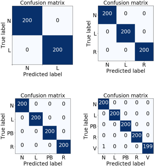
Confusion matrix of the beats classification for the proposed model in this study. 200 beats for each type of beat were considered in this experiment
We also obtained classification results using the pre-trained weight of fine-tuned modified VGG16 and CWT scalogram to understand whether the classification performance was affected by different input dimensions of ECG beat segments. We observed that for the input ECG segment dimension of 2.2, 2.3, 2.4, 2.5 s the test results remained the same, see Table 3. This indicates the proposed model can also classify ECG beat segments of slightly different dimensions very accurately.
Table 3.
Classification results obtained using pretrained weight of fine-tuned VGG16 with proposed customized classifier layers and CWT scalogram. The model was tested with the scalogram prepared with ECG beat-segments of various lengths
| Beat segments length (s) | Acc (%) | AUC | Se (%) | Sp (%) |
|---|---|---|---|---|
| 2 | 99.2 | 0.995 | 99.2 | 99.8 |
| 2.1 | 99.8 | 0.9988 | 99.8 | 99.95 |
| 2.2 | 99.9 | 0.9994 | 99.9 | 99.98 |
| 2.3 | 99.9 | 0.9994 | 99.9 | 99.98 |
| 2.4 | 99.9 | 0.9994 | 99.9 | 99.98 |
| 2.5 | 99.9 | 0.9994 | 99.9 | 99.98 |
| 2.6 | 99.3 | 0.9956 | 99.3 | 99.83 |
| 2.7 | 97.2 | 0.9825 | 97.2 | 99.3 |
| 2.8 | 93.5 | 0.9594 | 93.5 | 98.34 |
We also evaluated the proposed CWT-based fine-tuned model performance using ECG beats collected from the American Heart Association (AHA) Ventricular Arrhythmia ECG Database [44] and the Lobachevsky University Electrocardiography Database [45]. We used a total of 228 PVC (V type) beats obtained from the ‘0001’ and ‘0201’ files of the AHA database. The original ECG signals from the first channel were resampled to 360 Hz to keep the consistency of the classifier’s input before obtaining the scalogram. We collected 1431 normal (N) ECG beats from the lead ii from the Lobachevsky University Electrocardiography Database, which was also resampled to 360 Hz before obtaining the scalogram. The proposed CWT based fine-tuned model was tested with the new test set consisted of 1431, 200, 200, 200, and 228 samples for N, L, R, PB, and V beat types, respectively. An accuracy of 99.91%, F1 Macro of 99.90%, F1 Micro of 99.91%, sensitivity/recall of 99.83%, a specificity of 99.95%, ROC macro 99.89%, and ROC micro of 99.94% were obtained from the proposed model.
The contributions of the frequency components in ECG beats for classification are described as the SHAP value of the input image. Figure 8 shows the SHAP value on the scalogram, where the red colors on the time-frequency representation of the ECG signal indicate their positive contributions for being correctly separated from other beats. The figure shows that the 5–15 Hz frequency band is the most important for Left Bundle Branch Block beat (L), which can be considered as the distinguishable feature of it from the other ECG beats. For Right Bundle Branch Block beat (R), a small frequency band, 10 Hz to 14 Hz, is significant for classification. A vast range of frequency bands, 4 Hz to 100 Hz, in Paced Beat (PB) ECG arrhythmia is an important feature. A very lower band frequency, 2 Hz to 8 Hz, is the crucial frequency feature in Premature Ventricular Contraction (V) ECG beat.
Fig. 8.

SHAP values and frequency mapping in the time domain ECG. The beat on the top-left corner shows left bundle branch block beat (L) and its significant frequency contents based on the SHAP value in CWT-based scalogram. Bottom-left corner beat is a right bundle branch block beat (R) in which 10 Hz to 14 Hz frequency band is the key feature. On the top-right corner, paced beat (PB) shows 4 Hz to 100 Hz frequencies are notable. On the bottom-right corner, premature ventricular contraction (V) beat has very small range of frequency range, 2 Hz to 8 Hz, which resulted in high classification accuracy; thus distinct feature than other beats
Both the obtained beat classification results and the information about the characteristics frequency components in ECG beat can be used to produce test reports for patient treatment and managements.
Discussion
In this paper, the CWT feature of five classes of ECG beats collected from the MIT-BIH arrhythmia database was classified in order to measure the performance of the proposed deep CNN based classifier. The model also evaluated with the HHT feature of the same ECG arrhythmia. Later, we measured the SHAP value of the scalogram features to obtain the significant frequency components in the ECG beats which resulted in the highest classification accuracy. The observed frequency bands in the ECG may have some practical applications including monitoring the development of cardiac disease and monitoring the effectiveness of ongoing treatment.
Understanding the critical features of ECG beats in the frequency domain can be helpful for a deeper understanding of cardiac arrhythmias and their classification. Arrhythmia classification has shaped a center of consideration for academia and medical practitioners.
In this work, CWT is considered as the time-frequency representation (scalogram) of the ECG signal. Due to the non-stationary and non-linear nature of the ECG signal Morlet wavelet function has been used in this study. In the wavelet transform domain, the latent dynamics in frequency components of the ECG signal were more apparent than the standard time domain. We also evaluated the proposed classifier with spectral images of ECG beat segments obtained from the HHT, a modern signal-to-image conversion technique. The CWT scalogram over-performed the HHT spectrum in all the cases. Our proposed model coupled with scalogram demonstrated an accuracy of 100%, sensitivity of 100%, specificity of 100% and AUC of 100% for all the test cases of the datasets DB I, DB II, and DB III, and accuracy of 99.90%, sensitivity of 99.90%, specificity of 99.98% and AUC of 99.94% for the test cases of the DB IV dataset; thus, the model can be used as a powerful tool for assisting medical practitioners to diagnosis ECG arrhythmia.
We compared the classification accuracy obtained at previous studies to see the power of VGG16 and CWT scalogram in ECG beats classification. The proposed method, VGG16 based CNN with customized classifier layers model, showed superior performance compared to other studies that categorized similar beats from the same dataset, see Table 4.
Table 4.
The classification performance comparison of proposed methodology with some very recently published deep learning based existing methods
| Types of ECG beats | Literature | Feature | Classifiers | Se (%) | Sp (%) | Acc (%) |
|---|---|---|---|---|---|---|
| 2 (VT, VF) | Acharya et al. [25] | Time domain feature | CNN | 95.32 | 91.04 | 93.18 |
| 2 | Saninno et al. [27] | RR intervals | Deep learning | 99.52 | ||
| 2 (N, V) | Inan et al. [22] | WT and timing interval | Neural Network | 95.16 | ||
| 2 | Mathew et al. [28] | simple features | Deep belief network | 95.57 | ||
| 2 (N, L) | OUR STUDY | CWT t-f representation | VGG16 CNN | 100 | 100 | 100 |
| 3 (Normal, R, PB) | Isin et al. [33] | R-T interval | CNN | 92 | ||
| 3 (N, L, R) | Rai et al. [46] | Discrete Wavelet Transform (DWT) | Multilayer Probabilistic Neural Network (MPNN) | 99.01 | 99.53 | 99.07 |
| 3 (AF, A.Flut., VF) | Acharya et al. [29] | Time domain | CNN | 98.09-99.13 | 81.44–93.13 | 92.5–94.9 |
| 3 (N, L, R) | Jambukia et al. [30] | R peak and QRS complex | PSO-FFNN | 99.41 | ||
| 3 (N, L, R) | OUR STUDY | CWT t-f representation | VGG16 CNN | 100 | 100 | 100 |
| 4 | Gler et al. [47] | DWT coefficients | NN | 97.78 | 96.94 | |
| 4 | Taji et al. [48] | time domain | restricted Boltzman Machine | 73.1–100 | 75–99.5 | |
| 4 (N, L, R, PB) | Jambukia et al. [30] | R peak and QRS complex | PSO-FFNN | 98.68 | ||
| 4 | Wu et al. [38] | CWT based image | CNN | 97.56 | 99.19 | 97.56 |
| 4 (N, L, R, PB) | OUR STUDY | CWT t-f representation | VGG16 CNN | 100 | 100 | 100 |
| 5 | Kiranyaz et al. [49] | time domain | CNN | 64.4-95.9 | 98.1–99.5 | 96.6–99 |
| 5 | Acharya et al. [31] | time domain | CNN | 96.01 | 91.64 | 93.47 |
| 5 (N, L, R, V, A) | Oh et al. [50] | time domain | CNN and LSTM | 97.50 | 98.70 | 98.10 |
| 5 (N, L, R, PB, V) | OUR STUDY | CWT t-f representation | VGG16 CNN | 99.90 | 99.98 | 99.90 |
Bold texts indicate significant results
To improve the two-class arrhythmia classification accuracy, several machine and deep learning techniques like CNN, neural network, deep belief network have been used [22, 25, 27, 28]. Our proposed technique shows higher classification accuracy compared to those previous studies. The over performances of the proposed technique can be attributed to the appropriate deep learning model and CWT scalogram time-frequency input features which perfectly capture distinguishing frequency components in ECG beats.
In order to classify normal (N), left bundle branch block (L), and right bundle branch block (R) beats, some studies [30, 46] employed multilayer probabilistic neural network (MPNN) and PSO-CNN with the discrete wavelet transform (DWT), and R peak and QRS complex features. Our proposed model coupled with scalogram obtained at least 0.56% improved classification accuracy than the existing studied methods. In the case of four and five class classification, the customized VGG16 coupled with CWT scalogram input shows better classification than previous studies [30, 50]. All of these comparisons of the proposed technique with previous studies show the suitability of using the proposed model and CWT scalogram images for automated ECG beats classification.
The time-frequency power distribution over the frequencies is changed in the ECG arrhythmia beats [51–53]. The high frequency and power in the Ischemic cardiomyopathy ECG signal QRS complex are discovered [54]. We used SHAP to identify and visualize the wavelet coefficient in the scalogram and mapped that coefficient to the frequency in the ECG beats. We have found that the frequency components between 5 Hz and 18 Hz in the QRS complex of the previous beat of the left bundle block beat (L), between 5 Hz and 15 Hz in the QRS complex of L type arrhythmia beat, and between 5 Hz and 15 Hz in the QRS complex of next beat are significant. In the L type beats, we have found a lower band of the frequencies responsible for differentiating them from other beats. Similarly, for the right bundle branch block beat (R) lower band frequencies are responsible for differentiating them from other beats. A very small range of frequencies, from 10 Hz to 14 Hz, are most significant in the R beats. Immediately before and after the R beat, 5 Hz to 16 Hz frequencies are notable frequency features. In the premature ventricular contraction (V) beats, a very lower frequency band 2 Hz to 8 Hz, played a positive role for achieving excellent classification performance, thus frequency band of 2 Hz to 8 Hz in V beat is significant. In contrast to other beats, Paced Beat (PB) showed a frequency band with a very high range, 4 Hz to 100 Hz, responsible for the achieved classification accuracy.
The notable key features of this study are as follows: 1) it uses a single operation in the preprocessing stage, signal-to-image conversion which reduces preprocessing time and efforts. 2) the proposed CNN-based model shows very prominent results in ECG beat classification 3) The novel idea of using SHAP to identify frequency features in ECG beats.
Although we used the ECG dataset that is collected from 35 subjects, the main limitation of this study lies in not using different databases. Training the same proposed model with various databases, the statistical significance of characteristics frequency components in ECG beats need to be performed. However, based on the obtained results of this study, the proposed systems can be used in either stand-alone or cloud based automated ECG arrhythmia detection systems for cardiovascular disease diagnosis, patient treatment and managements.
Conclusion
In this paper, we have proposed an adopted VGG16-based CNN using the time-frequency representation of the ECG signal for cardiac arrhythmia classification. We have also identified frequency features in ECG that resulted in high classification accuracy. The results show 100% accuracy for two, three, and four class beat classification cases, and 99.90% for five class case. The VGG16-based CNN has proven to be effective and useful for heartbeat classification. We found that certain frequency components in the ECG were discriminative and helped the classifier distinguish between the ECG beats. In some beats low frequencies were responsible for different classification from other beats while in others it was higher frequency components that mainly determined the between-beat differences. Thus this CNN model could be useful for the diagnosis of the cardiovascular conditions and could be used by the health practitioners and clinicians.
Compliance with ethical standards
Conflict of interest
The authors declare that they have no conflict of interest.
Ethical approval
We have used publicly available data in our experiment. Therefore we do not need any ethical consent for this study.
Footnotes
Publisher's Note
Springer Nature remains neutral with regard to jurisdictional claims in published maps and institutional affiliations.
Contributor Information
Md. Rashed-Al-Mahfuz, Email: ram@ru.ac.bd
Mohammad Ali Moni, Email: m.moni@unsw.edu.au.
Pietro Lio’, Email: pl219@cam.ac.uk.
Sheikh Mohammed Shariful Islam, Email: shariful.islam@deakin.edu.au.
Shlomo Berkovsky, Email: shlomo.berkovsky@mq.edu.au.
Matloob Khushi, Email: matloob.khushi@sydney.edu.au.
Julian M. W. Quinn, Email: j.quinn@garvan.org.au
References
- 1.Benjamin EJ, Muntner P, Sommer MB. Heart disease and stroke statistics-2019 update: a report from the American heart association. Circulation. 2019;139(10):e56–e528. doi: 10.1161/CIR.0000000000000659. [DOI] [PubMed] [Google Scholar]
- 2.Narain SY, Kumar SSS, Kumar RA. Bioelectrical signals as emerging biometrics: issues and challenges; 2012. p. 2012.
- 3.Mohamed EAB, Dong GL, Makki AA, Gyeong MY, Eun-jong C, Jang-whan B, Myeong CC, Keun HR. Highlighting the current issues with pride suggestions for improving the performance of real time cardiac health monitoring. In: International Conference on Information Technology in Bio-and Medical Informatics, pp 226–233. Springer, 2010.
- 4.Shweta HJ, Vipul KD, Harshadkumar BP. Classification of ecg signals using machine learning techniques: a survey. In: 2015 International Conference on Advances in Computer Engineering and Applications, pp. 714–721. IEEE, 2015.
- 5.Rajendra AU, Paul JK, Kannathal N, Lim CM, Suri JS. Heart rate variability: a review. Med Biol Eng Comput. 2006;44(12):1031–51. doi: 10.1007/s11517-006-0119-0. [DOI] [PubMed] [Google Scholar]
- 6.Marwa MAH, Mohamed IE, Ahmed F. Computer aided diagnosis of cardiac arrhythmias. In: 2006 International Conference on Computer Engineering and Systems, pp. 262–265. IEEE, 2006.
- 7.De Chazal P, O’Dwyer M, Reilly RB. Automatic classification of heartbeats using ecg morphology and heartbeat interval features. IEEE Trans Biomed Eng. 2004;51(7):1196–206. doi: 10.1109/TBME.2004.827359. [DOI] [PubMed] [Google Scholar]
- 8.Terrill F, David HW. A minicomputer system for direct high speed analysis of cardiac arrhythmia in 24 h ambulatory ecg tape recordings. IEEE Trans Biomed Eng. 1980;12:685–693. doi: 10.1109/TBME.1980.326593. [DOI] [PubMed] [Google Scholar]
- 9.Coast Douglas A, Stern Richard M, Cano Gerald G, Briller SA. An approach to cardiac arrhythmia analysis using hidden markov models. IEEE Trans Biomed Eng. 1990;37(9):826–36. doi: 10.1109/10.58593. [DOI] [PubMed] [Google Scholar]
- 10.Lin K-P, Chang WH. Qrs feature extraction using linear prediction. IEEE Trans Biomed Eng. 1989;36(10):1050–5. doi: 10.1109/10.40806. [DOI] [PubMed] [Google Scholar]
- 11.Farid M, Yakoub B. Classification of electrocardiogram signals with support vector machines and particle swarm optimization. IEEE Trans Inf Technol Biomed. 2008;12(5):667–77. doi: 10.1109/TITB.2008.923147. [DOI] [PubMed] [Google Scholar]
- 12.Ge D, Srinivasan N, Krishnan SM. Cardiac arrhythmia classification using autoregressive modeling. Biomed Eng. 2002;1(1):5. doi: 10.1186/1475-925X-1-5. [DOI] [PMC free article] [PubMed] [Google Scholar]
- 13.Mishra AK, Raghav S. Local fractal dimension based ecg arrhythmia classification. Biomed Signal Process Control. 2010;5(2):114–23. doi: 10.1016/j.bspc.2010.01.002. [DOI] [Google Scholar]
- 14.Ali K, Ataollah E. Classification of electrocardiogram signals with support vector machines and genetic algorithms using power spectral features. Biomed Signal Process Control. 2010;5(4):252–63. doi: 10.1016/j.bspc.2010.07.006. [DOI] [Google Scholar]
- 15.Linh TH, Osowski S, Stodolski M. On-line heart beat recognition using hermite polynomials and neuro-fuzzy network. IEEE Trans Instrum Meas. 2003;52(4):1224–311. doi: 10.1109/TIM.2003.816841. [DOI] [Google Scholar]
- 16.Martis RJ, Chakraborty C, Ray AK. A two-stage mechanism for registration and classification of ecg using gaussian mixture model. Pattern Recognit. 2009;42(11):2979–88. doi: 10.1016/j.patcog.2009.02.008. [DOI] [Google Scholar]
- 17.Abdelhamid D, Latifa H, Naif A, Farid M. A wavelet optimization approach for ecg signal classification. Biomed Signal Process Control. 2012;7(4):342–9. doi: 10.1016/j.bspc.2011.07.001. [DOI] [Google Scholar]
- 18.Martis RJ, Muthu RKM, Chakraborty C, Pal S, Sarkar D, Mandana KM, Ray AK. Automated screening of arrhythmia using wavelet based machine learning techniques. J Med Syst. 2012;36(2):677–88. doi: 10.1007/s10916-010-9535-7. [DOI] [PubMed] [Google Scholar]
- 19.Hamid K, Majid M. A comparative study of dwt, cwt and dct transformations in ecg arrhythmias classification. Expert Syst Appl. 2010;37(8):5751–7. doi: 10.1016/j.eswa.2010.02.033. [DOI] [Google Scholar]
- 20.Yu HH, Palreddy S, Tompkins WJ. A patient-adaptable ecg beat classifier using a mixture of experts approach. IEEE Trans Biomed Eng. 1997;44(9):891–900. doi: 10.1109/10.623058. [DOI] [PubMed] [Google Scholar]
- 21.Jiang W, Kong SG. Block-based neural networks for personalized ecg signal classification. IEEE Trans Neural Netw. 2007;18(6):1750–61. doi: 10.1109/TNN.2007.900239. [DOI] [PubMed] [Google Scholar]
- 22.Inan OT, Giovangrandi L, Kovacs GTA. Robust neural-network-based classification of premature ventricular contractions using wavelet transform and timing interval features. IEEE Trans Biomed Eng. 2006;53(12):2507–15. doi: 10.1109/TBME.2006.880879. [DOI] [PubMed] [Google Scholar]
- 23.Martis RJ, Rajendra AU, Mandana KM, Ray AK, Chakraborty C. Application of principal component analysis to ecg signals for automated diagnosis of cardiac health. Expert Syst Appl. 2012;39(14):11792–800. doi: 10.1016/j.eswa.2012.04.072. [DOI] [Google Scholar]
- 24.Martis RJ, Rajendra AU, Mandana KM, Ray AK, Chakraborty C. Cardiac decision making using higher order spectra. Biomed Signal Process Control. 2013;8(2):193–203. doi: 10.1016/j.bspc.2012.08.004. [DOI] [Google Scholar]
- 25.Rajendra AU, Fujita H, Shu LO, Raghavendra U, Tan JH, Adam M, Gertych Arkadiusz HY. Automated identification of shockable and non-shockable life-threatening ventricular arrhythmias using convolutional neural network. Fut Gen Comput Syst. 2018;79:952–9. doi: 10.1016/j.future.2017.08.039. [DOI] [Google Scholar]
- 26.De Chazal P, Reilly RB. A patient-adapting heartbeat classifier using ecg morphology and heartbeat interval features. IEEE Trans Biomed Eng. 2006;53(12):2535–43. doi: 10.1109/TBME.2006.883802. [DOI] [PubMed] [Google Scholar]
- 27.Sannino G, De Pietro G. A deep learning approach for ecg-based heartbeat classification for arrhythmia detection. Fut Gen Comput Syst. 2018;86:446–55. doi: 10.1016/j.future.2018.03.057. [DOI] [Google Scholar]
- 28.Mathews SM, Kambhamettu C, Barner KE. A novel application of deep learning for single-lead ecg classification. Comput Biol Med. 2018;99:53–62. doi: 10.1016/j.compbiomed.2018.05.013. [DOI] [PubMed] [Google Scholar]
- 29.Rajendra AU, Hamido FO, Lih S, Hagiwara Y, Tan JH, Adam M. Automated detection of arrhythmias using different intervals of tachycardia ecg segments with convolutional neural network. Inf Sci. 2017;405:81–90. doi: 10.1016/j.ins.2017.04.012. [DOI] [Google Scholar]
- 30.Jambukia Shweta H, Dabhi Vipul K, Prajapati HB. Ecg beat classification using machine learning techniques. Int J Biomed Eng Technol. 2018;26(1):32–533. doi: 10.1504/IJBET.2018.089255. [DOI] [Google Scholar]
- 31.Rajendra AU, Shu LO, Hagiwara Y, Tan JH, Adam M, Gertych A, Tan RS. A deep convolutional neural network model to classify heartbeats. Comput Biol Med. 2017;89:389–96. doi: 10.1016/j.compbiomed.2017.08.022. [DOI] [PubMed] [Google Scholar]
- 32.Rajendra AU, Fujita H, Shu LO, Hagiwara Y, Tan JH, Adam M. Application of deep convolutional neural network for automated detection of myocardial infarction using ecg signals. Inf Sci. 2017;415:190–8. [Google Scholar]
- 33.Ali I, Selen O. Cardiac arrhythmia detection using deep learning. Procedia Comput Sci. 2017;120:268–75. doi: 10.1016/j.procs.2017.11.238. [DOI] [Google Scholar]
- 34.Rajendra AU, Fujita H, Shu LO, Hagiwara Y, Tan JH, Adam M, Tan RS. Deep convolutional neural network for the automated diagnosis of congestive heart failure using ecg signals. Appl Intell. 2019;49(1):16–27. doi: 10.1007/s10489-018-1179-1. [DOI] [Google Scholar]
- 35.Karen S, Andrew Z. Very deep convolutional networks for large-scale image recognition. 2014. arXiv preprint arXiv:1409.1556
- 36.Moody George B, Mark RG. The impact of the mit-bih arrhythmia database. IEEE Eng Med Biol Mag. 2001;20(3):45–50. doi: 10.1109/51.932724. [DOI] [PubMed] [Google Scholar]
- 37.R Mark, G Moody. Mit-bih database and software catalog, 1997.
- 38.Ziqian W, Xujian F, Cuiwei Y. A deep learning method to detect atrial fibrillation based on continuous wavelet transform. In: 2019 41st Annual International Conference of the IEEE Engineering in Medicine and Biology Society (EMBC), pp. 1908–1912. IEEE, 2019. [DOI] [PubMed]
- 39.Norden EH, Zheng S, Steven RL, Manli CW, Hsing HS, Quanan Z, Nai-Chyuan Y, Chi CT, Henry HL. The empirical mode decomposition and the hilbert spectrum for nonlinear and non-stationary time series analysis. Proc R Soc Lond Ser A Math Phys Eng Sci. 1998;454(1971):903–995. doi: 10.1098/rspa.1998.0193. [DOI] [Google Scholar]
- 40.Scott M L, Su-In L. A unified approach to interpreting model predictions. In I. Guyon, U. V. Luxburg, S. Bengio, H. Wallach, R. Fergus, S. Vishwanathan, R. Garnett, editors, Advances in Neural Information Processing Systems 30, pp. 4765–4774. Curran Associates, Inc., 2017.
- 41.Gabriel E, Joseph DJ, Pascal S, Scott L, Su-In L. Learning explainable models using attribution priors. 2019. arXiv preprint arXiv:1906.10670
- 42.Mukund S, Ankur T, Qiqi Y. Axiomatic attribution for deep networks. In: Proceedings of the 34th International Conference on Machine Learning-Volume 70, pp. 3319–3328. JMLR. org, 2017.
- 43.François C et al. Keras. https://github.com/fchollet/keras, 2015.
- 44.Ary LG, Luis ANA, Leon G, Jeffrey MH, Plamen CI, Roger GM, Joseph EM, George BM, Chung-Kang P, Stanley HE. Physiobank, physiotoolkit, and physionet: components of a new research resource for complex physiologic signals. Circulation. 2000;101(23):e215–e220. doi: 10.1161/01.cir.101.23.e215. [DOI] [PubMed] [Google Scholar]
- 45.Kalyakulina A, Yusipov II, Moskalenko VA, Nikolskiy AV, Kozlov AA, Kosonogov KA, Zolotykh NY, Ivanchenko MV. Lobachevsky university electrocardiography database (version 1.0. 0). PhysioNet, 2020.
- 46.Rai HM, Chatterjee K. A novel adaptive feature extraction for detection of cardiac arrhythmias using hybrid technique mrdwt & mpnn classifier from ecg big data. Big Data Res. 2018;12:13–22. doi: 10.1016/j.bdr.2018.02.003. [DOI] [Google Scholar]
- 47.Güler İnan, Übeylı Elif D. Ecg beat classifier designed by combined neural network model. Pattern Recognit. 2005;38(2):199–208.
- 48.Bahareh T, Adrian DCC, Shervin S. Classifying measured electrocardiogram signal quality using deep belief networks. In: 2017 IEEE International Instrumentation and Measurement Technology Conference (I2MTC), pp. 1–6. IEEE, 2017.
- 49.Serkan K, Turker I, Moncef G. Real-time patient-specific ecg classification by 1-d convolutional neural networks. IEEE Trans Biomed Eng. 2015;63(3):664–75. doi: 10.1109/TBME.2015.2468589. [DOI] [PubMed] [Google Scholar]
- 50.Shu LO, Ng EYK, Tan RS, Rajendra AU. Automated diagnosis of arrhythmia using combination of cnn and lstm techniques with variable length heart beats. Comput Biol Med. 2018;102:278–87. doi: 10.1016/j.compbiomed.2018.06.002. [DOI] [PubMed] [Google Scholar]
- 51.Gramatikov B, Brinker J, Yi-Chun S, Thakor NV. Wavelet analysis and time-frequency distributions of the body surface ecg before and after angioplasty. Comput Methods Progr Biomed. 2000;62(2):87–988. doi: 10.1016/S0169-2607(00)00060-2. [DOI] [PubMed] [Google Scholar]
- 52.Takano NK, Tsutsumi T, Suzuki H, Okamoto Y, Nakajima T. Time frequency power profile of qrs complex obtained with wavelet transform in spontaneously hypertensive rats. Comput Biol Med. 2012;42(2):205–12. doi: 10.1016/j.compbiomed.2011.11.009. [DOI] [PubMed] [Google Scholar]
- 53.Takeshi T, Yoshiwo O, Nami K-T, Daisuke W, Hiroshi S, Kazunori S, Kuniaki I, Toshiaki N. Time-frequency analysis of the qrs complex in patients with ischemic cardiomyopathy and myocardial infarction. IJC Heart Ves. 2014;4:177–87. doi: 10.1016/j.ijchv.2014.04.008. [DOI] [Google Scholar]
- 54.Ernest W, Reynolds JR, Muller B, Anderson GJ, Muller BT. High-frequency components in the electrocardiogram: a comparative study of normals and patients with myocardial disease. Circulation. 1967;35(1):195–206. doi: 10.1161/01.CIR.35.1.195. [DOI] [PubMed] [Google Scholar]