A Trial Emulation Approach for Policy Evaluations with Group-level Longitudinal Data

Supplemental Digital Content is available in the text.

Abstract

To limit the spread of the novel coronavirus, governments across the world implemented extraordinary physical distancing policies, such as stay-at-home orders. Numerous studies aim to estimate the effects of these policies. Many statistical and econometric methods, such as difference-in-differences, leverage repeated measurements, and variation in timing to estimate policy effects, including in the COVID-19 context. Although these methods are less common in epidemiology, epidemiologic researchers are well accustomed to handling similar complexities in studies of individual-level interventions. Target trial emulation emphasizes the need to carefully design a nonexperimental study in terms of inclusion and exclusion criteria, covariates, exposure definition, and outcome measurement—and the timing of those variables. We argue that policy evaluations using group-level longitudinal (“panel”) data need to take a similar careful approach to study design that we refer to as policy trial emulation. This approach is especially important when intervention timing varies across jurisdictions; the main idea is to construct target trials separately for each treatment cohort (states that implement the policy at the same time) and then aggregate. We present a stylized analysis of the impact of state-level stay-at-home orders on total coronavirus cases. We argue that estimates from panel methods—with the right data and careful modeling and diagnostics—can help add to our understanding of many policies, though doing so is often challenging.

To limit the spread of the novel coronavirus, governments across the world implemented extraordinary nonpharmaceutical interventions, such as closing nonessential businesses and imposing quarantines. The specific policies—and the decisions to lift them—varied widely, with particularly dramatic variation within the United States.¹ Learning about the impact of these policies is important both to inform future policy decisions and to construct accurate forecasts of the pandemic.

There are well-established epidemiologic methods for estimating the impact of an intervention that occurs in a single location and at a single time point, dating back to John Snow and the cholera epidemic in London.^2,3 Often known as difference-in-differences, the basic approach constructs counterfactual outcomes using group-level longitudinal data from the pre and postpolicy change time periods and from localities (e.g., states) that did and did not implement the policy. Variants of this approach are known as panel data methods and include event studies and comparative interrupted time series models.

There is no clear consensus in epidemiology, however, on how to proceed when many localities implement a policy over time, sometimes known as staggered adoption. Fortunately, epidemiologic researchers are well accustomed to handling similar complexities in studies of individual-level interventions, with decades of research on strong nonexperimental study designs, including methods that handle confounding and variation in timing of treatment across individuals. So-called target trial emulation emphasizes the need to carefully design a nonexperimental study in terms of inclusion and exclusion criteria, covariates, exposure definition, and outcome measurement—and the timing of all of those variables.^4,5

In this article, we argue that policy evaluations using panel data need to take a similarly careful approach, which we refer to as policy trial emulation, to study design. The main idea is to construct target trials separately for each treatment cohort (states that implement the policy at the same time) and then aggregate.⁶ We illustrate this approach by presenting a stylized analysis of the impact of state-level stay-at-home orders on total coronavirus cases. We believe this new connection to trial emulation is an important conceptual advance, though the underlying statistical methods we discuss are well established,⁷ and many of these points have been made in other contexts.⁸ We argue that estimates from panel methods—with the right data and careful modeling and diagnostics—can help add to our understanding of policy impacts. The underlying assumptions, however, are often strong and the application to COVID-19 anticontagion policies is particularly challenging.

The Elements of Policy Trial Emulation

We now describe key steps in conducting policy trial emulation that are necessary and obvious when designing a randomized trial and that are becoming more common in the design of nonexperimental studies. We argue that these steps are just as important when evaluating policies with aggregate longitudinal panel data.

We illustrate the key idea with a stylized policy evaluation: measuring the impact of US states adopting a shelter-in-place or stay-at-home policy on COVID-19 case counts. These orders urge or require citizens to remain at home except to conduct essential business, for example, grocery shopping or exercise; we use the New York Times Tracker to define policy enactment dates and obtain daily case counts.⁹ No institutional review board approval was needed for this use of publicly available aggregate data.

Defining Units and Exposures

First, we must have a consistent definition of the exposure. Specifically, there is only one form of treatment, and the outcome we see under a particular policy environment is equal to the potential outcome under that policy environment.¹⁰ For stay-at-home policies, different states enacted different requirements that broadly fall under this header, and the New York Times definition is just one. This introduces a trade-off. We could consider multiple types of treatment separately, such as closing schools versus closing nonessential businesses. However, this greatly expands the dimensionality of the specific exposure under consideration. Instead, we consider packaging interventions together, allowing for some variation in the specific implementation of the policy across units. As a result, the estimated effect averages over different policy-specific effects within the data, which may be less interpretable and may violate the consistency assumption.^8,11

Second, there is growing evidence that stay-at-home orders had only modest impacts on individual behavior—in many states, individuals reduced their mobility even in the absence of official policy changes.¹² Thus, we focus here on emulating an intent-to-treat (ITT) analysis, where individuals are randomized to treatment conditions, but the amount of treatment actually received (e.g., the dose) may differ across people. The ITT is often relevant for examining whether the policy is effective overall, regardless of specific implementation. If we had data on, for example, state-wide implementation of the policy or the level of adherence as determined by mobility measures, we could conduct an analysis analogous to a per-protocol effect, for example, estimating the effect of full policy implementation (i.e., all individuals following the stay-at-home guidelines).¹³ The trial emulation framework helps clarify the additional assumptions necessary for conducting a per-protocol analysis in this context.

Finally, an important complication is reasoning about interactions between units, for example, people with COVID-19 traveling across state lines and spreading infection. The trial emulation framework makes clear that we must pay close attention to this when defining our target trials: nearly all standard tools for policy evaluation assume no interference between units, that is, a state’s outcome only depends on that state’s intervention. Violations of this assumption, sometimes known as spillovers or contagion, complicate the definitions of units and exposures and can lead to bias.¹⁴ Understanding and explicitly modeling these violations is paramount when studying policies to control infectious diseases. For example, Holtz et al. use travel and social network information to account for spillovers across states.¹⁵ We refer interested readers to the large literature on observational causal inference with interference in general¹⁶ and on panel data methods in particular.¹⁷

Causal Contrasts of Interest

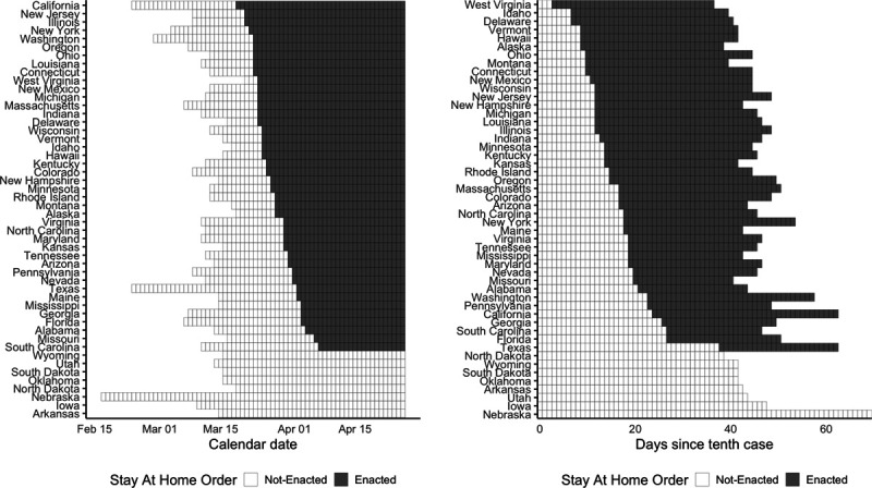
After defining units and exposures, the next step in the trial emulation framework is to define the estimand of interest.¹³ As discussed above, we focus on the ITT for treated states. Formally, let be an indicator that state i has a stay-at-home order at time t; and let be the corresponding observed outcome. We can express the causal quantity of interest via potential outcomes: 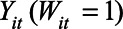is the outcome if the stay-at-home order is enacted, and 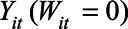is the outcome if the order is not enacted. The causal contrast of interest is then a difference between these potential outcomes, 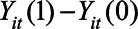, averaged over the states that implemented the policy and over posttreatment time periods.⁷

We also focus on the impact of “turning on” these policies, but of course states also turn them “off.” Just as in the individual exposure case, modeling individuals or locations turning exposures both on and off is complex. If that seems ambitious in a trial setting it is often even more ambitious in a nonexperimental context.

Defining Time Zero

The next step in trial emulation is to define time zero, that is, the point in time when individuals or states would have been randomized to treatment conditions.⁶ This is crucial for clearly distinguishing baseline (pretreatment) measures from outcomes (posttreatment): inappropriately conditioning on or selecting on posttreatment variables can cause as much bias (including immortal time bias) as can confounding.^5,18

In standard target trial emulation, time zero is often defined based on when individuals meet the specified eligibility criteria and is applied equally to both treated (exposed) and control (unexposed) units. In policy trial emulation, states are often eligible to implement a policy at any point, though this can also occur in standard target trial emulation.¹³ For treated states, we typically use the date the policy is enacted as time zero; for comparison states, however, analysts essentially need to identify the moment in time that a state was eligible to implement the policy but did not.

One option is to align states based on calendar time. For instance, below we focus on a target trial for states that enact stay-at-home orders on 23 March; we similarly set 23 March as time zero for the comparison states. In the COVID setting, however, we might instead want to measure time since the start of the pandemic in a specific location—given the sudden emergence of the pandemic, case counts are essentially undefined before this time. This presentation is in line with many of the epidemiologic models.¹⁹ We refer to this as case time and, as an illustration, index time according to the number of days since the 10th confirmed case.

Figure 1 (left panel) shows the timing of state-wide orders in calendar time beginning in mid-March with “early adopters” such as California, New Jersey, Illinois, and New York. State-wide orders continued through early April, with “late adopters” including Florida and Alabama. Several states, including Iowa and Arkansas, never enacted a state-wide order. Figure 1 (right panel) shows the timing in case time. From this perspective, early adopters, including West Virginia and Idaho, enacted stay-at-home orders within days of the tenth case, while California—the first state to enact a state-wide stay-at-home order—was relatively late to do so.

FIGURE 1.

Timing of state-wide stay-at-home orders, by calendar date (left) and case time (right). Calendar dates with fewer than 10 cases and case times after 26 April 2020 are blank.

The choice of time zero will depend on the context. In the COVID setting, case time is more consistent with models of infectious disease growth but is also more sensitive to the measurement error. Calendar time is more natural for accounting for “common shocks” to states, such as changes in federal policy, which occur on a specific date. Moreover, for some specific questions, such as impacts on employment outcomes, this distinction might not be relevant. For ease of exposition, we focus on calendar time in the main text and give analogous results in case time in the eAppendix; http://links.lww.com/EDE/B810.

Defining Outcomes

The next step in policy trial emulation is to clearly define the outcomes, both the measures themselves and their timing (t in the notation above). In a typical trial, an outcome might be something like mortality within 6 months. In our COVID case study we focus on two different outcome measures: (1) the (log) number of cases and (2) the log of the ratio of the current day’s case count to the previous day’s case count. The first is a measure of the cumulative effect, whereas the latter is a measure of the day-by-day changes in growth. We focus on log-transformed data because exponential disease growth can result in different preintervention trends on the raw outcome scale; we further discuss the risk of pre-trends below, and present results for raw case counts and case growth in the eAppendix; http://links.lww.com/EDE/B810. Data quality is also a key concern. Care needs to be taken to select outcomes that can be measured accurately; in particular, differential changes in the testing regime across states over time can lead to the illusion of an effect. Finally, we focus on outcomes that are measured at the aggregate (e.g., state) level, which is natural given the outcomes we examine. However, it is sometimes more reasonable to consider targeting a cluster- (rather than individual-) randomized trial in which treatment occurs at some aggregate level but outcome data are measured at the individual level.²⁰ The same trial emulation principles apply, and hierarchical modeling can be used to account for the multilevel structure.

Single Target Trial

We now describe a single target trial, and then turn to describing a sequence of nested target trials, which more fully captures the staggered adoption setting. Here, the goal is to estimate the impact for a single cohort of states that enact a stay-at-home order at the same time. For now, we focus on the five states that enacted the policy on 23 March 2020: Connecticut, Louisiana, Ohio, Oregon, and Washington.

Selecting Treated and Comparison States

In a randomized trial, researchers have the luxury of knowing that the exposed and unexposed units are similar on all baseline characteristics in expectation. This is not the case in nonexperimental studies such as policy evaluations. Thus, a key step in policy trial emulation is carefully selecting comparison units. We discuss statistical approaches for adjusting for differences in the next section.

An important consideration in selecting comparison units is the length of follow-up—once a comparison state enacts the treatment, it is no longer a useful comparison without strong modeling assumptions. Only 19 days passed between when the first and last states enacted stay-at-home orders, and if we compare the March 23 cohort to late-adopting states, we can observe effects for at most 10 days. In general, across cohorts, the longer the follow-up, the fewer available comparison states. The choice of time scale is especially important if comparing with late adopters, since a state might be a valid comparison in calendar time but not case time: Ohio’s stay-at-home order was enacted after California in calendar time but before California in case time.

Due to the lag between virus exposure, symptoms, and testing, we expect stay-at-home-orders to have delayed or gradual effects on the number of confirmed cases and case growth. How we define the start of the outcome time period (to then allow for different patterns of effects) is intimately related to the question of defining time zero, discussed above. Therefore, we compare the treated cohort to the eight never-treated states (Arkansas, North Dakota, South Dakota, Iowa, Nebraska, Oklahoma, Wyoming, and Utah), allowing for estimates of longer-term effects. In principle, we could use not-yet-treated states in the comparison group, dropping states from the comparison group at the time they enact the policy. However, the set of not-yet-treated states will change throughout the follow-up period. It may then be difficult to assess whether changes in outcomes are merely due to the changing composition of the comparison states. Additionally, for each set of comparison states at each follow-up period we will need to perform the diagnostic checks we describe below, potentially leading to an unwieldy number of diagnostics.

Estimating Treatment Effects

Once we have specified the target trial, the final stage is estimating the treatment effects and evaluating diagnostics for underlying assumptions. Although similar to standard trial emulation contexts in many ways, there are particular nuances and complications in the policy trial emulation setting given the longitudinal time series nature of the data and the relatively small number of units (e.g., 50 states). We illustrate this setup with simple estimators, especially the canonical difference-in-differences estimator; we discuss alternative estimators below.

Difference-in-differences Fundamentals

The basic building block of traditional panel data estimation is difference-in-differences. To build up to the difference-in-differences estimator, consider two possible (flawed) comparisons. We could compare the growth rate in the 23 March cohort before and after the stay-at-home order; The Table shows these growth rates, implying a decrease in the average log growth rate of 0.22, a reduction of about 20 percentage points. However, this simple comparison relies on the heroic assumption that the stay-at-home order is the only change affecting the growth rate following 23 March. Instead, we could directly compare the post 23 March growth rates for the two cohorts. From 23 March to 26 April, the treated states’ average log growth rate was 0.01 (1 percentage point) lower than the never treated states. Although this approach protects against shared “shocks” between the two cohorts—for example, changes in national policy or testing—it does not adjust for any differences in preintervention cases.

TABLE.

Average Log Growth Rate in Daily Case Counts for the 23 March Cohort and the Never-treated States (% Day-over-day Growth in Parentheses)

	Stay-at-Home Order		Difference
	Pre	Post
23 March cohort	0.31 (37%)	0.09 (10%)	−0.22 (−20%)
Never treated cohort	0.24 (27%)	0.10 (11%)	−0.14 (−12%)
Difference	+0.07 (+10%)	−0.01 (−1%)	−0.08 (−8%)

The preperiod is from 8 March to 22 March; the postperiod is from 23 March to 26 April.

Difference-in-differences combines these two approaches. First take the pre/post estimate of a decrease in the log growth rate by 0.22 in the 23 March cohort and compare it to a pre/post change in the never treated states, a decrease of 0.14. Taking the difference of these differences (hence difference-in-differences) yields an estimated reduction of the log growth rate by 0.08, or an 8 percentage point decrease in the growth rate (Table). Formally, this estimator is:

where and denote the pre and posttreatment average outcomes for cohort g, and denotes the never treated cohort.

The key to the differences-in-differences framework is a parallel counterfactual trends assumption: loosely, in the absence of any treatment, the trends for the treated cohort would be the same as the trends for the never-treated states, on average.^3,21 This assumption is inherently dependent on the outcome scale: if trends in log cases are equal, then trends in untransformed case numbers cannot also be equal. This assumption would be violated if there are anticipatory effects or time-varying confounding.

Anticipatory effects would imply that there are behavior changes before the state-wide shutdown, which would lead to bias since pretime zero measures would no longer truly be pretreatment. In the case of stay-at-home orders, there is strong evidence of such anticipatory behavior.¹²

Time-varying confounding would occur if the policy implementation decision making process depends on features other than baseline levels, that is, the average level of the outcome of interest in the baseline time period. For example, this would be violated if governors enacted stay-at-home orders in response to trends in case counts.

Finally, this approach relies entirely on outcome modeling and therefore differs from many common methods in epidemiology that instead model treatment, especially inverse probability of treatment weighting. Recent doubly robust implementations of difference-in-differences also incorporate inverse probability of treatment weighting and therefore rest on different assumptions than outcome modeling alone, including the positivity assumption that all units have a non-zero probability in being in each of the treatment conditions. Standard difference-in-difference models avoid positivity by instead relying on a parametric outcome model that potentially extrapolates across groups.^7,22

Diagnostics and Allowing Effects to Vary Over Time

The basic 2×2 table difference-in-differences estimator is a blunt tool: it estimates the effect averaged over the entire posttreatment period. By combining various 2×2 difference-in-differences estimators we can estimate how effects phase in after 23 March. First, we pick a common reference date, often the time period immediately preceding treatment (here, 22 March). Then for every other time period we estimate the 2×2 difference-in-differences relative to that date. Concretely, to estimate the effect k periods before and after treatment, we compute the 2×2 estimator:

where is the average for cohort g, periods before/after treatment. Figure 2 shows these estimates for the 23 March cohort, sometimes known as event study plots,²³ with uncertainty quantified via a leave-one-unit-out jackknife.⁷

FIGURE 2.

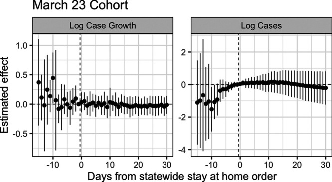
Difference-in-differences estimates for the effect of state-wide stay-at-home orders on log daily case growth and log cases for states in the March 23 cohort. Standard errors computed via jackknife.

This procedure has several advantages. First, this provides a diagnostic of the parallel trends assumption, similar in spirit to a balance check. The estimated difference-in-differences for (to the left of the dotted line) are “placebo” estimates of the impact of treatment k periods before treatment is enacted; if the parallel trends assumption holds, these should be close to zero. Although this is not a direct test of the actual assumption (since that involves counterfactual outcomes in the postpolicy period) assessing the preperiod trends can be thought of as a proxy for evaluating the assumption. As with all diagnostics, these are not a panacea: there is often limited statistical power to detect differences, and noisy estimates around zero do not absolve researchers from making the case for why the assumptions should hold.²⁴

As we see in Figure 2, in the week before 23 March the placebo estimates are near zero, but 2 weeks prior, there is higher variance and some evidence that growth rates were systematically higher in the treated cohort than the never-treated cohort, relative to March 22. For log cases, we see even more stark violations of the parallel trends assumption. Relative to the never-treated states, the March 23 cohort saw a larger increase in the number of cases, possibly evidence of time-varying confounding, although with such few units there is a large amount of uncertainty.

Finally, for , we estimate a different treatment effect for each period succeeding treatment, without imposing any assumptions on how we expect the treatment effects to phase in or out. From Figure 2 we see that in this single target trial there is insufficient precision to differentiate the effects from zero, let alone to distinguish a trend.

NESTED TARGET TRIALS

Selecting Units

We now estimate the overall average impact by repeating the trial emulation approach for all 42 states that eventually adopt a stay-at-home order. As above, the first step is to divide treated states into 17 cohorts based on adoption date. For each cohort, we then emulate a single target trial, selecting the same eight never-treated states as comparisons for every target trial. Finally, we aggregate results across these target trials.

These are nested target trials in the sense that each target trial can have a different starting point and length of follow-up.²⁵ This approach is sometimes known as stacking or event-by-event analysis in the econometrics literature.²⁶ The specific approach we implement here is equivalent to that in Abraham and Sun (2020)²³ and Callaway and Sant’Anna (2019)⁷ without any covariates.

Treatment Effect Estimation

In each single target trial, we estimate a series of two-period difference-in-differences estimates for that cohort as in the previous section. There are many ways to aggregate these estimates across cohorts.⁷ Here, we aggregate based on days since treatment (sometimes called event time):

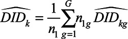where G is the total number of cohorts, is the number of treated units in cohort g, and is the total number of treated states. We refer to these as nested estimates.

Figure 3 shows the estimates from this approach, both for the effect on log case growth and on log cases. As with the single target trial, estimates to the right of zero are the treatment effects of interest, and estimates to the left of zero are “placebo estimates” of the impact of the treatment before the treatment itself. For the left panel (log case growth), the placebo estimates for the ten days before a state enacts a stay-at-home order are precisely estimated near zero; however, placebo effects prior to this are highly variable and show a downward trend over time. This suggests caution in interpreting the negative estimates to the right of zero. For the right panel (log cases), the placebo estimates are even more starkly different from zero, suggesting that this would not be an appropriate analysis and that the estimated effects are likely merely a reflection of these differential trends.

FIGURE 3.

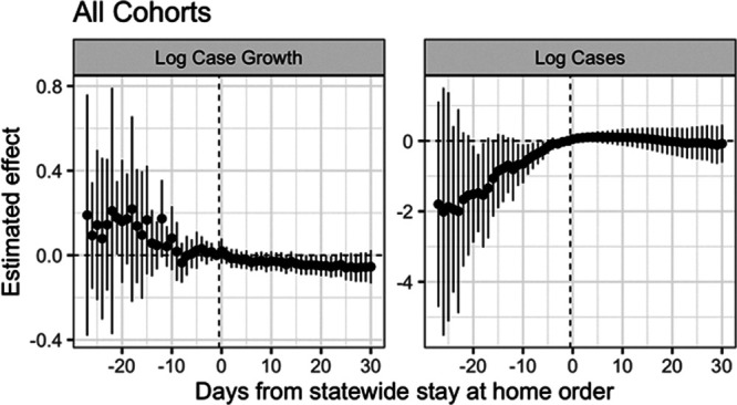
Nested estimates of the impact of state-wide stay-at-home orders on log cases and log case growth, in calendar time. Standard errors estimated with the jackknife.

DISCUSSION

In this article, we have introduced the idea of policy trial emulation as an approach for rigorous and careful policy evaluation, with a case study estimating the effects of stay-at-home orders during the beginning of the COVID-19 pandemic.

Epidemiologists regularly confront settings where multiple jurisdictions adopt a policy over time and the data available are aggregate longitudinal data on those and other jurisdictions. Policy trial emulation provides a principled framework for estimating causal effects in this setting.

The specific approach we advocate is not new; there is a growing literature in statistics and econometrics proposing robust methods for panel data. Here, we show that these ideas fit naturally into the trial emulation framework, especially the notion of aggregating across multiple target trials. As a result, we can leverage recent methodologic advances to enable more sophisticated estimation that allows for looser assumptions (e.g., parallel trends conditioned on covariates), including inverse propensity score weighting, doubly robust estimation, synthetic controls, and matching.^7,27–29 We could also impose stronger modeling assumptions on the time series, for example, a linear trend, such as in Comparative Interrupted Time Series.³⁰

One approach we caution against is the common practice of using regression to fit a longitudinal model to all the data, with fixed effects for state and time. As with individual data with time-varying treatments and confounders, naive regression models can mask important issues. In particular, it has been shown that the coefficient in this pooled model estimates a weighted average over all possible 2×2 difference-in-differences estimates, where the weights can be negative.²² Moreover, some of these estimates are not in the spirit of trial emulation, for example, by comparing two states that are entirely posttreatment. In practice, these complications mean that the sign of the estimated effect can be flipped relative to the nested estimate. Although some approaches, such as event study models, are less susceptible to this criticism,²³ we believe that the trial emulation framework we outline here is more transparent and less prone to error, partly by being explicit about all the causal contrasts.

The issues that we highlight are just some of many major challenges in estimating policy effects more generally, including: differences in the characteristics of states that do and don’t implement the policy and challenges in identifying the timing of effects, including limited statistical power.³¹ The COVID-19 pandemic adds additional complexities to these policy evaluations.⁸ For example, the disease transmission process, and the up to 2-week lag in the time from exposure to symptoms, makes it difficult to identify the precise timing of expected effects. Data on outcomes of interest are also limited or problematic; for example, case rates need to be considered within the context of the extent of testing.³² Finally, methods that do not account for spillovers and contagion are likely to be biased in this setting, and so properly addressing interference is a key methodologic and practical concern.

These issues—and the strong underlying assumptions—suggest caution in using difference-in-difference methods for estimating impacts of COVID-19 physical distancing policies. At the same time, the policy trial emulation framework suggests a rubric by which we can assess the quality of evidence presented in these studies. We anticipate that high-quality panel data methods will add to our understanding of these policies, especially when considered alongside other sources of evidence.

ACKNOWLEDGMENTS

We thank Elizabeth Stone, Ian Schmid, and Elena Badillo Goicoechea at Johns Hopkins for editorial help and constructive comments.

REFERENCES

- 1.The New York Times. See how all 50 states are reopening. Available at: https://www.nytimes.com/interactive/2020/us/states-reopen-map-coronavirus.html. Accessed 2 August 2020.
- 2.Wing C, Simon K, Bello-Gomez RA. Designing difference in difference studies: best practices for public health policy research. Annu Rev Public Health. 2018;39:453–469. [DOI] [PubMed] [Google Scholar]
- 3.Zeldow B, Hatfield LA. Confounding and regression adjustment in difference-in-differences. 2019https://arxiv.org/abs/1911.12185. [DOI] [PMC free article] [PubMed]
- 4.Danaei G, García Rodríguez LA, Cantero OF, Logan RW, Hernán MA. Electronic medical records can be used to emulate target trials of sustained treatment strategies. J Clin Epidemiol. 2018;96:12–22. [DOI] [PMC free article] [PubMed] [Google Scholar]
- 5.Dickerman BA, García-Albéniz X, Logan RW, Denaxas S, Hernán MA. Avoidable flaws in observational analyses: an application to statins and cancer. Nat Med. 2019;25:1601–1606. [DOI] [PMC free article] [PubMed] [Google Scholar]
- 6.Hernán MA, Robins JM. Per-protocol analyses of pragmatic trials. N Engl J Med. 2017;377:1391–1398. [DOI] [PubMed] [Google Scholar]
- 7.Callaway B, Sant’Anna Pedro HC. Difference-in-Differences with Multiple Time Periods. Forthcoming, Journal of Econometrics. 2019. Available at SSRN: https://ssrn.com/abstract=3148250 or doi: 10.2139/ssrn.3148250 [Google Scholar]
- 8.Goodman-Bacon A, Marcus J. Using difference-in-differences to identify causal effects of COVID-19 policies. Surv Res Methods. 2020;14:153–158. [Google Scholar]
- 9.The New York Times. Coronavirus (Covid-19) Data in the United States. Available at: https://github.com/nytimes/covid-19-data/blob/master/README.md. Accessed 2 August 2020.
- 10.Cole SR, Frangakis CE. The consistency statement in causal inference: a definition or an assumption? Epidemiology. 2009;20:3–5. [DOI] [PubMed] [Google Scholar]
- 11.Hernán MA. Does water kill? A call for less casual causal inferences. Ann Epidemiol. 2016;26:674–680. [DOI] [PMC free article] [PubMed] [Google Scholar]
- 12.Goolsbee A, Syverson C. Fear, lockdown, and diversion: comparing drivers of pandemic economic decline 2020. J Public Econ. 2021;193:104311. [DOI] [PMC free article] [PubMed] [Google Scholar]
- 13.Danaei G, Rodríguez LA, Cantero OF, Logan R, Hernán MA. Observational data for comparative effectiveness research: an emulation of randomised trials of statins and primary prevention of coronary heart disease. Stat Methods Med Res. 2013;22:70–96. [DOI] [PMC free article] [PubMed] [Google Scholar]
- 14.Halloran ME, Hudgens MG. Dependent happenings: a recent methodological review. Curr Epidemiol Rep. 2016;3:297–305. [DOI] [PMC free article] [PubMed] [Google Scholar]
- 15.Holtz D, Zhao M, Benzell SG, et al. Interdependence and the cost of uncoordinated responses to COVID-19. Proc Natl Acad Sci. 2020;117:19837–19843. [DOI] [PMC free article] [PubMed] [Google Scholar]
- 16.Ogburn EL, VanderWeele TJ. Vaccines, contagion, and social networks. Ann Appl Stat. 2017;11–12:919–948. [Google Scholar]
- 17.Di Gennaro D, Pellegrini G. Policy Evaluation in presence of interferences: a spatial multilevel DiD approach, CREI Università degli Studi Roma Tre. 2020; Working Paper. 0416. [Google Scholar]
- 18.Lévesque LE, Hanley JA, Kezouh A, Suissa S. Problem of immortal time bias in cohort studies: example using statins for preventing progression of diabetes. BMJ. 2010;340:b5087. [DOI] [PubMed] [Google Scholar]
- 19.Flaxman S, Mishra S, Gandy A, et al. Estimating the effects of non-pharmaceutical interventions on COVID-19 in Europe. Nature. 2020584:257–261. [DOI] [PubMed] [Google Scholar]
- 20.Page LC, Lenard MA, Keele L. The design of clustered observational studies in education. AERA Open. First published September 9, 2020. doi: 10.1177/2332858420954401 [Google Scholar]
- 21.Angrist JD, Pischke JS. Mostly Harmless Econometrics: An Empiricist’s Companion. 2009:Economics Books, Princeton University Press; 8769. [Google Scholar]
- 22.Goodman-Bacon A. Difference-in-differences with variation in treatment timing. National Bureau of Economic Research. Working Paper, 2018; 25018. Available at: https://www.nber.org/papers/w25018. Accessed 11 May 2021.
- 23.Sun L, Abraham S. Estimating dynamic treatment effects in event studies with heterogeneous treatment effects. 2020. Available at: https://arxiv.org/abs/1804.05785. Accessed 11 May 2021.
- 24.Rambachan A, Roth J. An Honest Approach to Parallel Trends. 2020. Available at: https://jonathandroth.github.io/assets/files/HonestParallelTrends_Main.pdf. Accessed 11 May 2021.
- 25.Hernán MA, Sauer BC, Hernández-Díaz S, Platt R, Shrier I. Specifying a target trial prevents immortal time bias and other self-inflicted injuries in observational analyses. J Clin Epidemiol. 2016;79:70–75. [DOI] [PMC free article] [PubMed] [Google Scholar]
- 26.Cengiz D, Dube A, Lindner A, Zipperer B. The effect of minimum wages on low-wage jobs. Q J Econ. 2019;13:1405–1454. [Google Scholar]
- 27.Arkhangelsky D, Athey S, Hirshberg DA, Imbens GW, Wager S. Synthetic difference in differences. 2019; Working Paper. Available at: https://arxiv.org/pdf/1812.09970.pdf. Accessed 11 May 2021. [Google Scholar]
- 28.Ben-Michael E, Feller A, Rothstein J. The augmented synthetic control method. 2020. Available at: https://arxiv.org/abs/1811.04170. Accessed 11 May 2021. [Google Scholar]
- 29.Daw JR, Hatfield LA. Matching and regression to the mean in difference-in-differences analysis. Health Services Res. 2018;53:4138–4156. [DOI] [PMC free article] [PubMed] [Google Scholar]
- 30.Health Policy Data Science Lab. Difference-in-Differences. 2019. Available at: https://diff.healthpolicydatascience.org. Accessed 11 May 2021.
- 31.Schell TL, Griffin BA, Andrew RM. Evaluating Methods to Estimate the Effect of State Laws on Firearm Deaths: A Simulation Study. 2018. RAND Corporation; Available at: https://www.rand.org/pubs/research_reports/RR2685.html. Accessed 11 May 2021. [Google Scholar]
- 32.Jagodnik JM, Ray F, Giorgi FM, Lachmann A. Correcting under-reported COVID-19 case numbers: estimating the true scale of the pandemic. 2020. medRxiv. 2020.03.14.20036178. [Google Scholar]
Associated Data
This section collects any data citations, data availability statements, or supplementary materials included in this article.