

Abstract
Transfer learning has been successfully used in the early diagnosis of Alzheimer’s disease (AD). In these methods, data from one single or multiple related source domain(s) are employed to aid the learning task in the target domain. However, most of the existing methods utilize data from all source domains, ignoring the fact that unrelated source domains may degrade the learning performance. Also, previous studies assume that class labels for all subjects are reliable, without considering the ambiguity of class labels caused by slight differences between early AD patients and normal control subjects. To address these issues, we propose to transform the original binary class label of a particular subject into a multi-bit label coding vector with the aid of multiple source domains. We further develop a robust multi-label transfer feature learning (rMLTFL) model to simultaneously capture a common set of features from different domains (including the target domain and all source domains) and to identify the unrelated source domains. We evaluate our method on 406 subjects from the Alzheimer’s Disease Neuroimaging Initiative (ADNI) database with baseline magnetic resonance imaging (MRI) and cerebrospinal fluid (CSF) data. The experimental results show that the proposed rMLTFL method can effectively improve the performance of AD diagnosis, compared with several state-of-the-art methods.
Keywords: Transfer learning, Multi-label learning, Feature learning, Alzheimer’s disease (AD)
Introduction
Alzheimer’s disease (AD) is the most common cause of dementia, which is a degenerative brain disease and characterized by a decline in memory, language, problem-solving and other cognitive skills that affects a person’s ability to perform everyday activities (Association 2015). This decline occurs because neurons and their connections in parts of the brain have been appeared progressive impairment. According to a recent report by Alzheimer’s Association, about 5.3 million Americans have AD, 5.1 million are age ≥ 65 years, and approximately 200,000 are age < 65 years and have Mild Cognitive Impairment (MCI), known as a prodromal stage of AD (Association 2015).
In recent years, much effort has been made to design computer-aided diagnosis systems, to allow early interventions that may prevent or delay the onset of AD/MCI. Especially, the prediction of whether an MCI subject will progress to AD (i.e., Progressive MCI, PMCI) or not (i.e., Stable MCI, SMCI) within a period is particularly important in practice. In the last decades, neuroimaging has been successfully used to investigate the characteristics of neurodegenerative progression in the spectrum from normal controls (NCs) to AD. For example, Magnetic Resonance Imaging (MRI) scans (Chao et al. 2010; Chetelat et al. 2005; deToledo-Morrell et al. 2004; Misra et al. 2009; Risacher et al. 2009) can measure the structural brain atrophy, and have been widely applied to the early diagnosis of MCI (Liu et al. 2016b). Cerebrospinal fluid (CSF) levels of Aβ42, total-tau (t-tau), and phosphor-tau (p-tau) have also been considered as effective biomarkers in tracking MCI progression (Bouwman et al. 2007; Davatzikos et al. 2011; Lehmann et al. 2012; Vemuri et al. 2009a, b). Recently, many machine learning methods have been proposed to fuse multi-modal biomarkers for the diagnosis of MCI, which generally achieve better learning performances than the conventional methods using single-modal biomarkers (Cheng et al. 2015a; Davatzikos et al. 2011; Dukart et al. 2016; Hao et al. 2016; Jie et al. 2015; Liu et al. 2014, 2017; Suk et al. 2014; Westman et al. 2012; Zhang and Shen 2012a, b; Zhang et al. 2011).
However, a major challenge in multi-modal biomarker based methods is that there are often limited samples and a large number of features, called the small-sample-size problem. To address this problem, many studies focus on feature learning for reducing the feature dimensionality (Cheng et al. 2015b; Eskildsen et al. 2013; Jie et al. 2015; Liu et al. 2014; Ota et al. 2015; Ye et al. 2012; Zhang and Shen 2012a; Zhou et al. 2013; Zhu et al. 2014, 2015). For instance, in Zhang and Shen 2012a, a multi-task learning method is proposed for fusing MRI, fluorodeoxyglucose positron emission tomography (FDG-PET), and CSF biomarkers. Then, a multi-task feature learning strategy is used for multi-modal feature selection in AD/MCI diagnosis (Jie et al. 2015; Liu et al. 2014; Zhu et al. 2014). However, in these studies, the training samples are often obtained from one particular learning domain, ignoring data in the other related learning domains. To enhance the generalization capability of models, several studies (Cheng et al. 2017, 2015a, b; Filipovych and Davatzikos 2011; Schwartz et al. 2012; Young et al. 2013) have utilized data from related learning domains for the model training in a target domain in a transfer learning manner. The basic idea is utilizing the knowledge learned from one or more source domains to aid the learning task in a target domain (Duan et al. 2012; Pan and Yang 2010; Yang et al. 2007), with the assumption that these source domains are related to the target domain. These studies suggested that the transfer learning methods using multi-modal biomarkers can improve AD/MCI classification performance. However, previous transfer learning based studies (Cheng et al. 2017, 2015a, b) directly used data from all source domains to aid the learning task in the target domain, without considering the negative effects of unrelated source domains. To address this issue, in this paper, we develop a robust multi-label transfer feature learning (rMLTFL) model to simultaneously capture a common set of features among multiple relevant domains and identify the unrelated source domains.
On the other hand, since AD is the progressive impairment of neurons, there are small differences between early AD patients and NC in neuroimaging. This phenomenon is more pronounced in patients with PMCI and SMCI, and thus the true class labels for subjects could be ambiguous. However, in practice, physicians often label one subject in a binary manner (i.e., belonging to the category of patients or not), and hence we assume that there could be errors in the human annotated class labels for subjects. Inspired by the recent error-correcting output coding strategy (Liu et al. 2016a; Pujol et al. 2006), we propose to transform the original binary class label of a particular subject into a multi-bit label coding vector to avoid the negative effects caused by ambiguous class labels.
In this paper, we consider four classification tasks for the early diagnosis of AD/MCI, including the classification of (1) AD vs. NC, (2) MCI vs. NC, (3) AD vs. MCI, and (4) PMCI vs. SMCI. We also illustrate the relationship between the target domain and the corresponding multi-source domains in Fig. 1. For instance, in AD vs. NC classification, we regard data in the other three tasks (i.e., MCI vs. NC, AD vs. MCI, and PMCI vs. SMCI) as source domains. We then develop a multi-label prediction approach for subjects in the target domain with the aid of multi-source domains, via a transfer learning technique (Pan and Yang 2010). Finally, we propose a robust multi-label transfer feature learning (rMLTFL) model to select a common set of features among multiple relevant domains, by using the multi-bit coding vector as the label for each training subject. The proposed method is evaluated on 406 subjects from the Alzheimer’s Disease Neuroimaging Initiative (ADNI) with both MRI and CSF data. The experimental results demonstrate that the proposed method can further improve the performance of early diagnosis of the AD, compared to several state-of-the-art methods.
Fig. 1.

Illustration of relationships between target domain and multiple source domains in four classification tasks
Materials
The Alzheimer’s Disease Neuroimaging Initiative (ADNI) unites researchers with study data as they work to define the progression of Alzheimer’s disease. ADNI researchers collect, validate and utilize data such as MRI and PET images, genetics, cognitive tests, CSF and blood biomarkers as predictors of the disease. Data from the North American ADNI’s study participants, including Alzheimer’s disease patients, mild cognitive impairment subjects and elderly controls, are available from this site (http://adni.loni.usc.edu/). In addition, ADNI researchers collect several types of data from study volunteers throughout their participation in the study. Data collection is performed using a standard set of protocols and procedures to eliminate inconsistencies. This information is available for free to authorized investigators through the Image Data Archive (IDA).
Alzheimer’s Disease (AD) is an irreversible neurodegenerative disease that results in a loss of mental function due to the deterioration of brain tissue. It is the most common cause of dementia among people over the age of 65, affecting an estimated 5.3 million Americans, yet no prevention methods or cures have been discovered. For more information about Alzheimer’s disease, visit the Alzheimer’s Association. The goal of the ADNI study is to track the progression of the disease using biomarkers to assess the brain’s structure and function over the course of four disease states. The ADNI study will assess participants in the following stages:
CN (i.e., Normal Aging/Cognitively Normal), from ADNI1 and ADNI2, CN participants are the control subjects in the ADNI study. They show no signs of depression, mild cognitive impairment or dementia.
SMC (i.e., Significant Memory Concern), from ADNI2, SMC participants score within the normal range for cognition (or Clinical Dementia Rating, i.e., CDR = 0) but indicate that they have a concern, and exhibit slight forgetfulness. The informant does not equate this as progressive memory impairment nor considers this as consistent forgetfulness.
MCI (i.e., Mild Cognitive Impairment), from ADNI1 and ADNI2, MCI participants have reported a subjective memory concern either autonomously or via an informant or clinician. However, there are no significant levels of impairment in other cognitive domains, essentially preserved activities of daily living and there are no signs of dementia. MCI is a prodromal stage of the AD, where some MCI patients will convert to AD, i.e., progressive MCI (PMCI), and other MCI patients remain stable, i.e., stable MCI (SMCI). Levels of MCI (early or late) are determined using the Wechsler Memory Scale Logical Memory II.
AD (i.e., Alzheimer’s disease), from ADNI1 and ADNI2, AD participants have been evaluated and meet the National Institute of Neurological and Communicative Disorders and Stroke and the Alzheimer’s Disease and Related Disorders Association (NINCDS/ADRDA) criteria for the probable AD.
Here, ADNI2 has added a new cohort, the Significant Memory Concern (SMC). Subjective memory concerns have been shown to be correlated with a higher likelihood of progression, thereby minimizing the stratification of risk among normal controls and addressing the gap between healthy elderly controls and MCI. The key inclusion criteria that distinguish the Significant Memory Concern cohort are a self-report significant memory concern from the participant, quantified by using the Cognitive Change Index and the Clinical Dementia Rating (CDR) of zero.
In this work, we focus on using the ADNI1 database with baseline MRI and CSF data. Specifically, the structural MR scans were acquired that participants were previously scanned using either a 1.5T or 3T scanner. Imaging for ongoing participants occurs annually, within two weeks before or two weeks after the in-clinic assessments. We downloaded the baseline CSF Aβ42, t-tau and p-tau data from the ADNI web site (http://adni.loni.usc.edu/) in December 2009. The CSF collection and transportation protocols are provided in the ADNI procedural manual on http://www.adni-info.org. The more detailed description can be found in (Zhang et al. 2011). In this study, CSF Aβ42, CSF t-tau and CSF p-tau are used as the features.
Method
In this section, we first briefly introduce our proposed feature learning method, and then present the image pre-processing and feature extraction methods from MR images. Finally, we present our proposed robust multi-label transfer feature learning (rMLTFL) model, as well as an optimization algorithm for solving the proposed objective function.
Overview
In Fig. 2, we illustrate the proposed feature learning framework for the early diagnosis of AD/MCI. Specifically, our framework consists of three main components, i.e., (1) image pre-processing and feature extraction, (2) robust multi-label transfer feature learning (rMLTFL), and (3) brain disease classification using SVM. As shown in Fig. 2, we first pre-process all MR images, and extract features from MR images. Then, we select informative features via the proposed rMLTFL method. We finally train an SVM classifier using the dimension-reduced data in the target domain for the diagnosis of AD and MCI.
Fig. 2.

Illustration of our proposed robust multi-label transfer feature learning (rMLTFL) framework for early diagnosis of AD. Here, X is the feature matrix, and Y denotes the multi-bit label coding matrix with each row denoting the label for a particular subject
Image preprocessing and feature extraction
All MR images were pre-processed by following the pipeline in (Zhang et al. 2011), then extracted the regions-of-interest (ROIs)-based features. Specifically, the pre-processing flow is showed in Fig. 3. After registration, each subject image was labeled and gets the 93 manually-labeled ROIs. Then, for each of 93 ROIs, we computed its GM tissue volume as a feature. As a result, for each subject, we have a 93-dimensional feature vector for representing it. For multi-modal data fusion, we simply concatenated the features of MRI and CSF into a long feature vector.
Fig. 3.
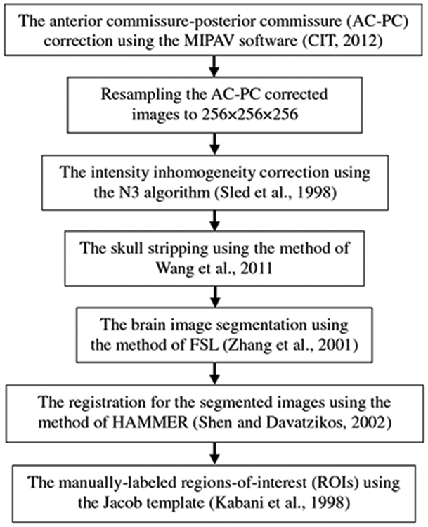
The pre-processing flow of MR images
Robust multi-label transfer feature learning (rMLTFL)
To reasonably utilize more data from multiple related source domains (multi-source domains for short), we propose a robust Multi-Label Transfer Feature Learning (rMLTFL) model which simultaneously captures a common set of features among multiple relevant domains and identifies the unrelated domains. Specifically, the proposed rMLTFL model consists of two key components: (1) multi-bit label coding matrix construction via the technique of transfer learning, and (2) the proposed robust multi-label transfer feature learning (rMLTFL) model and an optimization algorithm for solving the objective function.
Multi-bit label coding
As a progressive disease, there may be slight differences between early AD patients and NC on neuroimaging. Hence, the class label for one subject could be ambiguous. Unlike previous studies that label one subject in a binary manner (i.e., patient or not), we propose to transform the original binary class label of a particular subject into a multi-bit label coding vector with the aid of data from multi-source domains, inspired by the recent error-correcting output coding strategy (Liu et al. 2016a; Pujol et al. 2006). Also, previous studies have suggested that the learning task of AD diagnosis is related to the learning task of MCI diagnosis (Cheng et al. 2015b; Coupé et al. 2012; Da et al. 2014; Filipovych and Davatzikos 2011; Westman et al. 2013; Young et al. 2013), and transfer learning methods improve the classification accuracy of AD and MCI (Cheng et al. 2015a, b; Filipovych and Davatzikos 2011; Schwartz et al. 2012; Young et al. 2013). Hence, in this work, we adopt data in multi-source domains for generating the multi-bit label coding vector for each subject in a transfer learning manner.
Specifically, the multi-bit label coding matrix for subjects is generated via the technique of transductive transfer learning (Pan and Yang 2010). Throughout the whole paper, we denote the target domain as X with true label yt and those k source domains as S = {S1, S2, … , Sk}. For clarity, we illustrate in Fig. 4 the process of using multi-source domain data for the generation of multi-bit label matrix. As can be seen from Fig. 4, there are three steps for achieving the multi-bit label matrix. In the first step, we treat each of multi-source domain data as the training set, and data in the target domain as the testing set. In the second step, we train a support vector machine (SVM) classifier using data from each source domain, and achieve k SVM classifiers. Finally, we feed a subject xp in the target domain to each of k SVMs, and obtain the estimated label vector . Given xp in the target domain and its estimated labels, we construct its estimated multi-bit label matrix . In this way, for a particular subject in the target domain, we have a k-bit vector as its new label. Considering the true label vector yt, we denote as the multi-bit label coding matrix for all subjects in the target domain, where n is the number of subjects in the target domain.
Fig. 4.

Illustration of the generation process for multi-bit label coding matrix with the aid of data from multi-source domains. We first treat each of multi-source domain data as the training set, and data in the target domain as the testing set. We then train k SVMs based on data in k source domains, and apply the learned SVMs to each testing subject (e.g., xp) to get the estimated class labels (i.e., ). For each subject in the target domain, we finally combine k predicted labels as a multi-bit label matrix
Robust multi-label transfer feature learning model (rMLTFL)
Inspired by the robust multi-task feature learning (Gong et al. 2012), we propose a robust multi-label transfer feature learning model (rMLTFL), which can simultaneously capture a common set of features among multiple learning domains and identify the unrelated domains. In the following subsections, we first introduce the formulation of rMLTFL model and then employ the accelerated gradient descent (AGD) method (Gong et al. 2012; Nesterov 2004, 2007) to solve the optimization problem of rMLTFL model. In the end of this section, we present a two-stage procedure on the feature selection step of using rMLTFL model and call this two-stage procedure as 2S-rMLTFL.
Formulation
Assume that we have a training set from the target domain, with the i-th element and its human-annotated class label, where n denotes the number of training samples and d is the number of training sample feature. Different from the conventional feature learning models using only a single response variable, our proposed rMLTFL model can learn a weight matrix from the target-domain training set X and its multi-bit label coding matrix Y. In order to identify the unrelated domains and select the common set of features among multiple learning domains simultaneously, the weight matrix W is decomposed into the sum of two components P and Q. We make use of two L2,1-norm based regularization terms on P and Q to exploit relationships among multiple domains. Also, in order to simultaneously learn the weight vector learning of wt and each , we introduce an L2-norm regularizer (i.e., ) in the proposed objective function, which is used for capturing the correlation information between the true label vector yt and each estimated multi-bit label vector via square distance minimization. Formally, our rMLTFL model is formulated as:
| (1) |
where the first term is the empirical loss of the training data, the term ∥·∥F denotes the Frobenius norm for a matrix and the term QT denotes the transpose of a matrix Q. The second term is used to encourage the similarity between the distance from the predicted target-domain label Xwt to each predicted multi-bit label (i.e., ) and the distance from the true target-domain label yt to each estimated multi-bit label (i.e., ). For clarity, we illustrate the meaning of the second term in Eq. (1) in Fig. 5. The third term ∥P∥2,1 is used to capture the shared features among multiple domains; the last term ∥QT∥2,1 is utilized to discover the unrelated domains, and then the weight matrix W is the sum of two components P and Q that is illustrated in Fig. 6. In addition, parameters of λ1, λ2 and λ3 are nonnegative and be used to control these three regularization terms. It is worth noting that the third term in Eq. (1) is the well-known group Lasso penalty which restricts the rows of the optimal solution P* to have all zero or nonzero elements (Argyriou et al. 2008). In this way, all related domains would select a common set of features. Similarly, we introduce the fourth regularization term based on the group Lasso penalty on columns of Q to discover these unrelated source domains. In this way, we can select features corresponding to non-zero rows in P for feature selection, and identify those unrelated or less informative source domains corresponding to non-zero columns in Q.
Fig. 5.
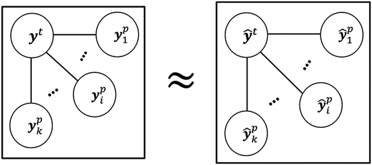
Illustration of measuring the similarity among residual vectors in Eq. (1). Each node represents a column vector of the target-domain label or the multi-bit label that estimated by multi-source domain data, edges represent the distance between nodes. Here, and
Fig. 6.

Illustration of weight matrix decomposition for rMLTFL, where squares with white background denote zero entries. Here, is a weight matrix, and the weight matrix of W is decomposed into the matrix sum of two components P and Q. Each column is corresponding to a specific domain. There are four domains, where the second domain is an unrelated domain
The proposed rMLTFL model is different from the robust multi-task feature learning (rMTFL) model in (Gong et al. 2012). Specifically, we propose a new regularization term to capture the correlation of inter-multi-bit label coding term (i.e., ) in the model of rMLTFL. In addition, these two models (i.e., rMTFL and rMLTFL) have different sources of training data. That is, training data from multiple learning tasks are used the input for rMTFL, while only the single learning task data is used for the model training of rMLTFL. In brief, our proposed rMLTFL model can utilize the correlation information between inter-multi-bit label coding and inter-samples, but rMTFL does not considered the correlation between training samples from multiple learning tasks.
Optimization algorithm
To solve the optimization problem of Eq. (1), we employ the accelerated gradient descent algorithm (Gong et al. 2012; Nesterov 2004, 2007). To be specific, the proposed objective function in Eq. (1) can be transformed as follows:
| (2) |
where is a (k + 1) × k sparse matrix and defined as follows: Hi,j = 1 if i = 1, Hi,j = −1 if i = j + 1, and Hi,j = 0 otherwise.
To solve the formulation in Eq. (2) efficiently, we decompose the objective function in Eq. (2) into two parts, i.e., a differential term L(P,Q) and a non-differential term R(P,Q), as follows:
| (3) |
where L(P,Q) is the loss function and R(P,Q) is the regularization term. Since the loss function L(P,Q) is differentiable, we can compute its gradient function. However, the term of R(P,Q) is non-differential function, it cannot compute the gradient function of R(P,Q). Some studies employ the accelerated gradient descent method to solve the kind of optimization problem (Chen et al. 2009; Liu et al. 2009a, b). Specifically, we can obtain the first order Taylor expansion of L(P,Q) at(), with the squared Euclidean distance between (P,Q) and () being treated as the regularization term as follows:
| (4) |
The accelerated gradient descent method is used in this work, which generates the solution at the t-th iteration (t ≥ 1) by computing the following proximal operator (Liu et al. 2009b, c):
| (5) |
where , and , for t ≥ 1. The coefficient βt is with respect to the convergence of the algorithm, and then we set βt = (bt−1 − 1)/bt, where b0 = 1, for t ≥ 1 (Gong et al. 2012). In addition, the coefficient γt (t ⩾ 1) is set as γt = 2γt−1, and γ0 is set as the lower bound of L. According to the research work of Gong et al. 2012, we set the lower bound of L as L ⩾ min in this paper.
Due to the decomposable property of Eq. (5), we can cast Eq. (5) into the following two separate proximal operator problems:
| (6) |
where and are the partial derivatives of with respect to and at . The above proximal operator problems admit closed form solutions as follows:
| (7) |
where (u(t))i denote the i-th row of Ut, denote the j-th column of Vt , and , . Finally, these initialization of variables (i.e., , ) can be obtained from the study of Gong et al. 2012.
Two-stage procedure for rMLTFL (2S-rMLTFL)
Our proposed rMLTFL model can be directly used for feature selection. Specifically, for the procedure of feature selection, we select those features corresponding to non-zero rows in the optimal solution P* that is learned by rMLTFL model with the AGD algorithm. In this way, all multi-bit label vectors are included in model training of rMLTFL so that those unrelated domains should make negative effects for classification.
To avoid negative effects of those unrelated domains and inspired by the work of 2S-rMTFL (Gong et al. 2012), we also present a two-stage procedure for rMLTFL and illustrate this process in Fig. 7. Specifically, we first run the rMLTFL on the target domain training set X with its multi-bit label coding matrix Y and then observe that certain multi-bit label vectors can be selected and identified as unrelated label vectors. Then, we remove these unrelated label vectors, obtaining a new multi-bit label coding matrix . Finally, we run rMLTFL on this ‘clean’ multi-label feature learning problem. We call this two-stage procedure as 2S-rMLTFL. In this paper, we use the procedure of 2S-rMLTFL for feature selection.
Fig. 7.
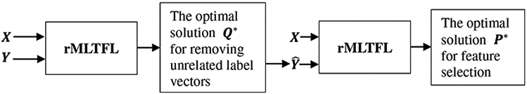
Illustration of our proposed two-stage feature selection procedure using rMLTFL (called 2S-rMLTFL). X represents the target domain training data and its multi-bit label coding matrix Y, is a new multi-bit label coding matrix that is learned by rMLTFL model
Results
In this section, we first describe experimental settings in our experiments. Then, we show the classification results on the ADNI database by comparing our proposed method with several state-of-the-art methods. In addition, we illustrate the most discriminative features identified by our proposed method.
Experimental settings
We use 406 subjects (102 AD, 192 MCI, and 112 NC) with baseline MRI and CSF data from the ADNI database. It is worth noting that, for all 192 MCI subjects, during the 24-month follow-up period, 86 MCI subjects converted to AD (PMCI for short) and 106 MCI subjects remained stable (SMCI for short). In addition, we consider four binary classification tasks, i.e., AD (+ 1) vs. NC (−1) classification, MCI (+ 1) vs. NC (−1) classification, AD (+ 1) vs. MCI (−1) classification, and PMCI (+ 1) vs. SMCI (−1) classification.
In all experiments, we adopt a 10-fold cross-validation strategy to partition the target domain data into training and testing subsets. To avoid the possible bias occurred during sample partitioning, we repeat this 10-fold cross-validation 10 times, and report the average performances in terms of area under the receiver operating characteristic curve (AUC), accuracy (ACC), sensitivity (SEN), and specificity (SPE).
We first compare the proposed rMLTFL method with a baseline method using the standard SVM (denoted as Baseline). Then, we compare rMLTFL with four state-of-the-art methods, including (1) Lasso (Tibshirani 1996), (2) MTFS (Liu et al. 2009b; Obozinski et al. 2006), (3) MLFS (Liu et al. 2009c), and (4) rMTFL (Gong et al. 2012). These methods are listed as follows.
Baseline: is diagramed in Fig. 8a, training data are only from the target domain, without any feature selection stage. The linear SVM with C = 1 is used as the classifier.
Lasso: (Tibshirani 1996) is diagramed in Fig. 8b, training data are only from the target domain, and the L1-norm based feature selection is performed before classification. Finally, a linear SVM is used for classification.
MLFS: Multi-Label Lasso feature selection (Liu et al. 2009c) is diagramed in Fig. 8c, training data are only from the target domain, and the target multi-label response matrix is computed by our proposed method of multi-bit label coding matrix construction. Then, the MLFS algorithm is used for feature selection, followed by a linear SVM classifier.
MTFS: Multi-Task Lasso feature selection (Liu et al. 2009b; Obozinski et al. 2006) is diagramed in Fig. 8d, training data are from both the target domain and multi-source domains, and the MTFS algorithm is conducted for feature selection before using linear SVM for classification.
rMTFL: robust Multi-Task Feature Learning (Gong et al. 2012) is diagramed in Fig. 8e. The rMTFL method is proposed in Gong et al. 2012. Besides the original rMTFL method, we further compare our method with its two-stage version, called 2S-rMTFL. Specifically, training data are from both the target domain and multi-source domains, we first run the rMTFL algorithm on the training set and observe that certain domains can be selected and identified as an unrelated domain. Then, we remove these unrelated domains, and only keep those related source domains. Finally, we run the rMTFL algorithm on this ‘clean’ multi-domain data for feature selection. The linear SVM is used for classification.
Fig. 8.
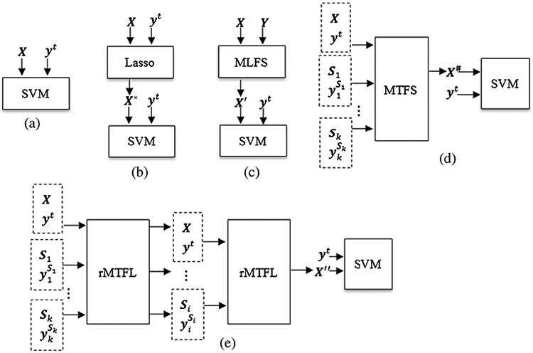
Illustration of five competing methods, X represents the target domain training data and its multi-bit label coding matrix Y, yt is the true label vector of target domain training data, S1, … , S1, … , Sk denote k source domains and their true label vectors , and X*, X′, X*, X″ denote dimension-reduced training data of target domain via procedures of Lasso, MLFS, MTFS and 2S-rMTFL respectively
The SVM is implemented using the LIBSVM toolbox (Chang and Lin 2001) with a linear kernel and a default value for the parameter C = 1. For the Lasso and MLFS methods, we adopt the SLEP toolbox (Liu et al. 2009c) to solve the optimization problem. There are multiple regularization parameters of these methods (including Lasso, MTFS, MLFS, rMTFL, and our proposed rMLTFL) to be optimized. All regularization parameters of these methods are chosen from the range of Z1 by a nested 10-fold cross-validation on the training data. Before training models, we normalized features by following (Zhang et al. 2011).
Comparison between rMLTFL and other methods
Table 1 shows the classification results achieved by six methods, including Baseline, Lasso, MTFS, MLFS, rMTFL, and the proposed rMLTFL method. Note that each value in Table 1 is the averaged result of the 10-fold cross validation. We also use DeLong’s method (DeLong et al. 1988) on the AUC between the proposed method and each of other five competing methods, and list the corresponding P-values in Table 1. In addition, we plot the ROC curves achieved by six methods in four classification tasks in Fig. 9.
Table 1.
Comparison of our proposed method (rMLTFL) and five state-of-the-art methods (Baseline, Lasso, MTFS, MLFS, and rMTFL) for four classification tasks
| Method | ACC | SEN | SPE | AUC | P-value |
|---|---|---|---|---|---|
| AD vs. NC | |||||
| Baseline | 0.887 | 0.881 | 0.892 | 0.960 | < 0.0001 |
| Lasso | 0.916 | 0.912 | 0.920 | 0.976 | < 0.0005 |
| MTFS | 0.916 | 0.912 | 0.919 | 0.972 | < 0.0005 |
| MLFS | 0.912 | 0.908 | 0.916 | 0.970 | < 0.0001 |
| rMTFL | 0.927 | 0.926 | 0.928 | 0.978 | < 0.005 |
| rMLTFL (Ours) | 0.952 | 0.952 | 0.953 | 0.983 | – |
| MCI vs. NC | |||||
| Baseline | 0.731 | 0.787 | 0.635 | 0.809 | < 0.0001 |
| Lasso | 0.765 | 0.814 | 0.681 | 0.832 | < 0.0001 |
| MTFS | 0.768 | 0.816 | 0.685 | 0.833 | < 0.0005 |
| MLFS | 0.761 | 0.810 | 0.675 | 0.830 | < 0.0001 |
| rMTFL | 0.783 | 0.836 | 0.677 | 0.840 | < 0.001 |
| rMLTFL (Ours) | 0.824 | 0.867 | 0.738 | 0.865 | – |
| PMCI vs. SMCI | |||||
| Baseline | 0.664 | 0.624 | 0.697 | 0.716 | < 0.0001 |
| Lasso | 0.711 | 0.676 | 0.739 | 0.790 | < 0.0005 |
| MTFS | 0.687 | 0.649 | 0.717 | 0.749 | < 0.0001 |
| MLFS | 0.707 | 0.672 | 0.735 | 0.757 | < 0.0001 |
| rMTFL | 0.731 | 0.725 | 0.734 | 0.794 | < 0.001 |
| rMLTFL (Ours) | 0.763 | 0.734 | 0.786 | 0.810 | – |
| AD vs. MCI | |||||
| Baseline | 0.657 | 0.506 | 0.738 | 0.696 | < 0.0001 |
| Lasso | 0.704 | 0.574 | 0.774 | 0.753 | < 0.0005 |
| MTFS | 0.712 | 0.585 | 0.780 | 0.742 | < 0.0001 |
| MLFS | 0.709 | 0.580 | 0.777 | 0.743 | < 0.0005 |
| rMTFL | 0.728 | 0.545 | 0.792 | 0.782 | < 0.001 |
| rMLTFL (Ours) | 0.767 | 0.614 | 0.818 | 0.820 | – |
ACC ACCuracy, SEN SENsitivity, SPE SPEcificity, AUC Area Under the receiver operating characteristic Curve
Fig. 9.

ROC curves of six different methods in four classification tasks
As can be seen from Table 1 and Fig. 9, we can have the following observations. First, for four binary classification problems, the proposed rMLTFL method consistently outperforms those five competing methods regarding all measures. Second, our proposed rMLTFL method and the rMTFL method outperform the other methods, which implies that removing unrelated domains can achieve better classification performance. Also, these results show our proposed assumption (that several unrelated domains often exist in multi-domain learning) is reasonable. Third, rMLTFL consistently achieves better classification performance than rMTFL, which suggests that our proposed regularization term on is useful in promoting classification performance. In addition, Lasso method slightly outperforms MLFS and MTFS methods in four binary classification problems, which implies that one or more unrelated domains will cause negative effects and restrict the improvement of classification performance. This further proves that the motivation of our approach (i.e., eliminating the negative effects of these irrelevant domains to further improve the diagnostic performance of AD and MCI) is reasonable.
Discussion
In this paper, we propose a robust multi-label transfer feature learning (rMLTFL) method for early diagnosis of AD, which can simultaneously capture a common set of features from the multi-source domain and target domain data and identify the unrelated domains. We evaluate the performance of our method on 406 subjects from the publicly available ADNI database and compare our method with state-of-the-art methods. The experimental results show that the proposed method can consistently and sub-stantially improve the performance of early diagnosis of AD.
Robust multi-label transfer feature learning
In the field of neuroimaging-based early diagnosis of AD, multi-task multi-model learning methods have been widely used for feature selection and classification (Cheng et al. 2015a, b; Dukart et al. 2016; Hao et al. 2016; Hinrichs et al. 2011; Jie et al. 2015; Liu et al. 2014; Suk et al. 2014; Wang et al. 2016; Ye et al. 2012; Zhang and Shen 2012a; Zhang et al. 2011; Zhu et al. 2014), showing improved performance in AD diagnosis. The multi-task learning is based on the assumption that all these learning tasks should enable correlation. However, one or several unrelated learning tasks often exist in multiple learning tasks, and most of the existing studies haven’t considered this case. On the other hand, there are small differences between early AD patients and NC on neuroimaging, especially slight differences between PMCI and SMCI patients, so we consider that some errors often exist in the true labels while labeling neuroimages. To avoid negative effects from unreliable class labels, we develop a multi-bit label coding method using the technique of transductive transfer learning. Also, we consider that one or several unrelated label vectors exist in the multi-label matrix. In this paper, we propose a robust multi-label transfer feature learning (rMLTFL) method that can simultaneously capture a common set of features among multi-label matrix and identify the unrelated label vectors. Different from multi-task learning, the rMLTFL method requires that data from multi-source domains are not used directly in model training. In Table 1 and Fig. 6, MTFS and rMTFL using multi-task learning are inferior to rMLTFL using multi-label learning for the classification performance, which implies that our proposed robust multi-label transfer learning is more suitable for early diagnosis of AD based on multi-source domain data.
There are three regularization parameters (i.e., λ1, λ2, λ3) in the proposed rMLTFL model. We further investigate the contribution of each regularization term by setting the respective parameters to be zero, and show the results in Table 2. For example, we set the regularization parameter λ1 as zero (i.e., λ1 = 0), which is used for evaluating the contribution of the first regularization term. As can be seen from Table 2, combining three regularization terms (i.e., λ1, λ2, λ3 > 0) can achieve better performance for early diagnosis of AD. These results suggest the importance of selecting unrelated domains and capturing structured information between the true label vector and the predicted multi-label vectors.
Table 2.
Comparison of our proposed rMLTFL method using different settings of regularization parameters
| Regularization parameter | AD vs. NC | MCI vs. NC | PMCI vs. SMCI | AD vs. MCI | ||||
|---|---|---|---|---|---|---|---|---|
| ACC | AUC | ACC | AUC | ACC | AUC | ACC | AUC | |
| λ1 = 0 | 0.928 | 0.974 | 0.792 | 0.851 | 0.737 | 0.795 | 0.727 | 0.768 |
| λ2 = 0 | 0.948 | 0.981 | 0.813 | 0.867 | 0.762 | 0.809 | 0.759 | 0.808 |
| λ3 = 0 | 0.920 | 0.971 | 0.784 | 0.834 | 0.729 | 0.786 | 0.719 | 0.764 |
| λ1, λ2, λ3 > 0 | 0.952 | 0.983 | 0.824 | 0.865 | 0.763 | 0.810 | 0.767 | 0.820 |
In this work, we use a square loss function in the rMLTFL model that is suitable for both regression and classification learning tasks. To evaluate the influence of different loss functions, we further compare rMLTFL with its variant (called rMLTFL_log). Different from rMLTFL that is a linear regression model, rMLTFL_log is a logistic regression model using a logistic loss function. The experimental results achieved by two competing methods (i.e., rMLTFL, and rMLTFL_log) are reported in Table 3. From Table 3, we can observe that the performance of rMLTFL_log with a logistic loss function is slightly superior to rMLTFL having a square loss function. We have further employed DeLong’s method (DeLong et al. 1988) on the AUC values achieved by rMLTFL and rMLTFL_log, and obtained p-values that are greater than 0.05 in four classification tasks (AD vs. NC, MCI vs. NC, PMCI vs. SMCI, and AD vs. MCI). This demonstrates that there is no statistically significant difference between the AUC values obtained by rMLTFL and rMLTFL_log between our proposed rMLTFL model (with a square loss function) and its variant rMLTFL_log with a logistic loss function.
Table 3.
Comparison between our proposed rMLTFL model (with a square loss function) and its variant rMLTFL_log with a logistic loss function
| Model | AD vs. NC | MCI vs. NC | PMCI vs. SMCI | AD vs. MCI | ||||
|---|---|---|---|---|---|---|---|---|
| ACC | AUC | ACC | AUC | ACC | AUC | ACC | AUC | |
| rMLTFL_log | 0.955 | 0.986 | 0.833 | 0.876 | 0.772 | 0.824 | 0.771 | 0.832 |
| rMLTFL | 0.952 | 0.983 | 0.824 | 0.865 | 0.763 | 0.810 | 0.767 | 0.820 |
Discriminative features detection
The proposed rMLTFL model can be used for identifying the most discriminative features (corresponding to ROIs), which are helpful for early diagnosis of AD in clinical practice. Since we adopt a 10-fold cross-validation strategy to evaluate the efficacy of rMLTFL model and the feature selection in each fold was performed only based on the current training set, the selected features could vary across different cross-validations. We thus define the most discriminative features based on the selected frequency of each feature among 10-fold cross-validation. In Tables 4 and 5, we list all selected features with the highest frequency of occurrence (i.e., each feature selected across all folds and all runs) by rMLTFL on concatenated multi-modal biomarkers (i.e., MRI + CSF) in four classification tasks. From Tables 4 and 5, we can observe that our proposed rMLTFL model successfully selects the most discriminative features, since the corresponding ROIs are known to be related to Alzheimer’s disease (Davatzikos et al. 2011; Eskildsen et al. 2013; Jie et al. 2015; Ye et al. 2012; Zhang and Shen 2012a; Zhang et al. 2011; Zhu et al. 2014). The features (i.e., t-tau and p-tau) that are from CSF biomarker are selected for four classification tasks, and brain regions that are related to early diagnosis of AD (e.g., amygdala, hippocampal formation, entorhinal cortex, uncus, peripheral cortex, and cuneus) are also selected from MRI biomarker, which imply that combining MRI and CSF biomarkers are able to provide complementary and discriminative information in the early diagnosis of AD.
Table 4.
The most discriminative features identified by the rMLTFL model for the classification tasks of AD vs. NC and AD vs. MCI
| AD vs. NC | AD vs. MCI |
|---|---|
| Middle frontal gyrus right | Precentral gyrus right |
| Lateral front-orbital gyrus right | Lateral front-orbital gyrus right |
| Angular gyrus right | Superior frontal gyrus right |
| Fornix left | Angular gyrus right |
| Middle frontal gyrus left | Fornix left |
| Uncus left | Posterior limb of internal capsule inc. Cerebral peduncle left |
| Occipital lobe WM left | Posterior limb of internal capsule inc. Cerebral peduncle right |
| Precentral gyrus left | Superior occipital gyrus right |
| Perirhinal cortex left | Middle frontal gyrus left |
| Amygdala right | Middle occipital gyrus right |
| Inferior temporal gyrus right | Middle temporal gyrus left |
| Lateral occipitotemporal gyrus left | Precentral gyrus left |
| Aβ42 | Lateral front-orbital gyrus left |
| t-tau | Inferior temporal gyrus left |
| p-tau | Lateral occipitotemporal gyrus right Entorhinal cortex right |
| Insula left | |
| Medial frontal gyrus right | |
| Middle temporal gyrus right | |
| Corpus callosum | |
| Amygdala right | |
| Inferior temporal gyrus right | |
| Superior temporal gyrus right | |
| Occipital pole left | |
| t-tau | |
| p-tau |
Table 5.
The most discriminative features identified by the rMLTFL model for the classification tasks of MCI vs. NC and PMCI vs. SMCI
| MCI vs. NC | PMCI vs. SMCI |
|---|---|
| Medial front-orbital gyrus right | Nucleus accumbens right |
| Middle frontal gyrus right | Anterior limb of internal capsule left |
| Lateral front-orbital gyrus right | Caudate nucleus right |
| Medial frontal gyrus left | Precuneus left |
| Uncus right | Postcentral gyrus left |
| Fornix left | Precentral gyrus left |
| Hippocampal formation right | Perirhinal cortex right |
| Cuneus left | Perirhinal cortex left |
| Lingual gyrus left | Inferior temporal gyrus right |
| Postcentral gyrus left | Aβ42 |
| Precentral gyrus left | t-tau |
| Superior occipital gyrus left | p-tau |
| Lateral occipitotemporal gyrus right Hippocampal formation left | |
| Medial occipitotemporal gyrus left | |
| Medial occipitotemporal gyrus right | |
| Thalamus right | |
| Occipital pole left | |
| Aβ42 | |
| t-tau | |
| p-tau |
In Table 4, there are nine features that are selected together for the classification tasks of AD vs. NC and AD vs. MCI, such as lateral front-orbital gyrus right, angular gyrus right, fornix left, middle frontal gyrus left, precentral gyrus left, amygdala right, inferior temporal gyrus right of MRI biomarker, and t-tau, p-tau of CSF biomarker, which indicate that those brain regions have been onset of the lesions in the stage of MCI (Davatzikos et al. 2011; Zhang et al. 2011). Also, there are four brain regions (i.e., lateral front-orbital gyrus right, fornix left, middle frontal gyrus right and precentral gyrus left) that are selected together for the classification tasks of AD vs. NC, and MCI vs. NC, which imply that the three brain regions are to shrink in early stage of AD (Davatzikos et al. 2011; Eskildsen et al. 2013; Zhang et al. 2011). In addition, those features (i.e., precentral gyrus left, perirhinal cortex left, inferior temporal gyrus right, Aβ42, t-tau, and p-tau) are selected together for the classification tasks of AD vs. NC and PMCI vs. SMCI, which show that CSF and brain atrophy are effective for early diagnosis of AD and also tracking of MCI progression. In a word, these conclusions suggest that brain structure and function have changed with the progression of AD. The common most discriminative features are existed in all four classification tasks, which validate that the four classification tasks are related to each other.
Unrelated source domains detection
Identifying one or several unrelated label vectors from all multi-bit label coding vectors is useful and novel work for our proposed rMLTFL model. Since multi-source domain data are used for the training of rMLTFL model, we consider that one or several unrelated source domains possible exist in multi-source domains. For identifying unrelated source domains, we use the rMLTFL model to select unrelated label vectors, and then those selected label vectors are corresponding to unrelated domains.
Specifically, we adopt the group Lasso penalty on the columns of Q to discover these unrelated label vectors, and then affirm corresponding unrelated domains via these zero columns in Q. Since we adopt a 10-fold cross-validation strategy to evaluate the efficacy of rMLTFL model and also the unrelated domain selection in each fold is performed only based on the current training set, the selected domains could vary across different cross-validations. Also, we repeat the 10-fold cross-validation with 10 times, in order to avoid the possible bias occurred during sample partitioning. Therefore, we record the ratio of each domain that is identified as the unrelated domain among ten folds in each classification task, with results shown in Table 6. Because the true label is rarely selected as unrelated domain (all selected ratios are under the 5%), we only list the selected ratios of unrelated source domains in Table 6.
Table 6.
The unrelated source domains identified by the rMLTFL model for four classification tasks
| Target Domain | Multi-source Domains | ||
|---|---|---|---|
| AD vs. NC | MCI vs. NC | PMCI vs. SMCI | AD vs. MCI |
| 75% | 43% | 22% | |
| MCI vs. NC | AD vs. NC | PMCI vs. SMCI | AD vs. MCI |
| 20% | 46% | 73% | |
| PMCI vs. SMCI | AD vs. NC | MCI vs. NC | AD vs. MCI |
| 17% | 75% | 48% | |
| AD vs. MCI | AD vs. NC | MCI vs. NC | PMCI vs. SMCI |
| 74% | 50% | 15% | |
As can be seen from Table 6, for the target domain of AD vs. NC, the source domain of MCI vs. NC is selected as unrelated domain in most cases (the selected ratio is 75%). For the target domain of MCI vs. NC, the source domain of AD vs. MCI is selected as unrelated domain in most cases (the selected ratio is 73%). For the target domain of PMCI vs. SMCI, the source domain of MCI vs. NC is selected as unrelated domain in most cases (the selected ratio is 75%). For the target domain of AD vs. MCI, the source domain of AD vs. NC is selected as unrelated domain in most cases (the selected ratio is 74%). Also, we provide results produced by rMLTFL and 2S-rMLTFL approaches in Table 7. These results suggest that one or several unrelated domains exist in the multi-source domains, and removing unrelated domains can improve the classification performance.
Table 7.
Comparison between the rMLTFL model using 2S-rMLTFL strategy (‘2S-rMLTFL’) and the rMLTFL model without using 2S-rMLTFL strategy (‘rMLTFL’)
| Method | AD vs. NC | MCI vs. NC | PMCI vs. SMCI | AD vs. MCI | ||||
|---|---|---|---|---|---|---|---|---|
| ACC | AUC | ACC | AUC | ACC | AUC | ACC | AUC | |
| rMLTFL | 0.921 | 0.973 | 0.786 | 0.835 | 0.732 | 0.789 | 0.721 | 0.767 |
| 2S-rMLTFL | 0.952 | 0.983 | 0.824 | 0.865 | 0.763 | 0.810 | 0.767 | 0.820 |
Extension for classifying SMCI and NC
In the early diagnosis of Alzheimer’s disease, recognition of MCI subject will progress to AD (i.e., PMCI) is becoming increasingly important. Therefore, we report classification results of classifying SMCI and PMCI in Table 1. In order to get a more accurate diagnosis of MCI, we would report classification results of classifying SMCI and NC with our proposed rMLTFL model that uses the 2S-rMLTFL strategy. Specifically, the target domain is the learning task of classifying SMCI (+ 1) and NC (−1), multi-source domains are four binary classification tasks, i.e., AD (+ 1) vs. NC (−1), MCI (+ 1) vs. NC (−1), AD (+ 1) vs. MCI (−1), and PMCI (+ 1) vs. SMCI (−1). First, we compute a multi-bit label coding matrix via the approach of multi-bit label coding matrix construction and then learn a common set of features by the rMLTFL model with 2S-rMLTFL strategy; the linear SVM is used for classification in the last step. In Table 8, we provide four performance measurements (i.e., ACC, SEN, SPE and AUC) and the P-value that is computed by DeLong’s method (DeLong et al. 1988) on the AUC between the proposed method and each of other five competing methods.
Table 8.
Comparison of our proposed method (rMLTFL) and five state-of-the-art methods (Baseline, Lasso, MTFS, MLFS, and rMTFL) for classifying SMCI and NC
| Method | ACC | SEN | SPE | AUC | P-value |
|---|---|---|---|---|---|
| Baseline | 0.646 | 0.634 | 0.655 | 0.708 | < 0.001 |
| Lasso | 0.684 | 0.673 | 0.693 | 0.752 | < 0.01 |
| MTFS | 0.695 | 0.685 | 0.704 | 0.752 | < 0.01 |
| MLFS | 0.691 | 0.681 | 0.700 | 0.747 | < 0.005 |
| rMTFL | 0.695 | 0.684 | 0.703 | 0.749 | < 0.005 |
| rMLTFL | 0.743 | 0.741 | 0.744 | 0.808 | – |
As can be seen from Table 8, the rMLTFL method consistently outperforms those five competing methods regarding all measurements. Moreover, there are several interesting observations as following: (1) classification results of MTFS and MLFS methods are slightly better than Lasso method, which indicates that multi-source domains are related to the target domain, and classification performance on target domain can be improved by the aid of multi-source domains; (2) classification results of rMTFL method are slightly inferior to MTFS method, which indicates that it is not able to select unrelated domains using the rMTFL method; (3) classification results of rMLTFL method are better than MTFS, MLFS, and rMTFL methods, which indicates that one or more unrelated domains are existed in multi-source domains, and extraction of correlation information among multi-bit label coding vectors is able to improve performance of classifying SMCI and NC.
Limitations
The current study is limited by several factors. First, our proposed method is based on the two modal (i.e., MRI + CSF) biomarkers from the ADNI database. In the ADNI database, many subjects also have more modal biomarkers, such as FDG-PET. Also, many status-unlabeled subjects can be used to extend our current method. In the future work, we will investigate whether adding more multi-modal and status-unlabeled data can further improve the performance. Second, for the preprocessing of MR images, our current study only uses ROI features, while previous studies have shown the effectiveness of cortical thickness in early diagnosis of AD (Cho et al. 2012; Cuingnet et al. 2011; Eskildsen et al. 2013; Querbes et al. 2009; Wee et al. 2013; Wolz et al. 2011). In the future work, we will consider extracting cortical thickness features from MR images and combine them with ROI based features for early diagnosis of AD.
Conclusion
In this paper, we propose a novel robust multi-label transfer feature learning (rMLTFL) framework for early diagnosis of AD, which simultaneously captures a common set of features among multiple relevant domains and identifies the unrelated domains. The main idea of our method is to exploit the multi-source domain data to improve classification performance in the target domain. Specifically, we first develop a method for multi-bit label coding using the technique of transductive transfer learning. Then, we propose a robust multi-label transfer feature learning (rMLTFL) model that can simultaneously utilize the multi-bit label coding vectors and the original class labels for subjects to capture a common set of features among multiple relevant domains and identify the unrelated domains. We evaluate our method on the baseline ADNI database with MRI and CSF data, and the experimental results demonstrate the efficacy of our method.
Acknowledgements
Data collection and sharing for this project was funded by the Alzheimer’s Disease Neuroimaging Initiative (ADNI) (National Institutes of Health Grant U01 AG024904). ADNI is funded by the National Institute on Aging, the National Institute of Biomedical Imaging and Bioengineering, and through generous contributions from the following: Abbott, AstraZeneca AB, Bayer Schering Pharma AG, Bristol-Myers Squibb, Eisai Global Clinical Development, Elan Corporation, Genentech, GE Healthcare, GlaxoSmithKline, Innogenetics, Johnson and Johnson, Eli Lilly and Co., Medpace, Inc., Merck and Co., Inc., Novartis AG, Pfizer Inc, F. Hoffman-La Roche, Schering-Plough, Synarc, Inc., as well as non-profit partners the Alzheimer’s Association and Alzheimer’s Drug Discovery Foundation, with participation from the U.S. Food and Drug Administration. Private sector contributions to ADNI are facilitated by the Foundation for the National Institutes of Health (http://www.fnih.org). The grantee organization is the Northern California Institute for Research and Education, and the study is coordinated by the Alzheimer’s Disease Cooperative Study at the University of California, San Diego. ADNI data are disseminated by the Laboratory for Neuron Imaging at the University of California, Los Angeles. This work was supported by the National Natural Science Foundation of China (Nos. 61602072, 61573023, 61732006, and 61473149), Chongqing Cutting-edge and Applied Foundation Research Program (Grant No. cstc2016jcyjA0063), Scientific and Technological Research Program of Chongqing Municipal Education Commission (Grant Nos. KJ1401010, KJ1601003, KJ1601015, KJ1710248, KJ1710257), NIH grants (AG041721, AG049371, AG042599, AG053867), Key Laboratory of Chongqing Municipal Institutions of Higher Education (Grant No. [2017]3), and Program of Chongqing Development and Reform Commission (Grant No. 2017[1007]).
Footnotes
Data used in preparation of this article were obtained from the Alzheimer’s Disease Neuroimaging Initiative (ADNI) database (http://adni.loni.usc.edu/). As such, the investigators within the ADNI contributed to the design and implementation of ADNI and/or provided data but did not participate in analysis or writing of this report. A complete listing of ADNI investigators can be found at: http://adni.loni.usc.edu/about/governance/principal-investigators/.
Z ∈ {0.000001, 0.00001, 0.0001, 0.0003, 0.0007, 0.001, 0.003, 0.005, 0.007, 0.01, 0.02, 0.03, 0.04, 0.05, 0.06, 0.07, 0.08, 0.09, 0.1, 0.2, 0.3, 0.4, 0.5, 0.6, 0.7, 0.8, 0.9}
References
- Argyriou A, Evgeniou T, & Pontil M (2008). Convex multi-task feature learning. Machine Learning, 73, 243–272. [Google Scholar]
- Association, A. s. (2015). 2015 Alzheimer’s disease facts and figures. Alzheimer’s & Dement, 11, 332–384. [DOI] [PubMed] [Google Scholar]
- Bouwman FH, Schoonenboom SNM, van der Flier WM, van Elk EJ, Kok A, Barkhof F, Blankenstein MA, & Scheltens P (2007). CSF biomarkers and medial temporal lobe atrophy predict dementia in mild cognitive impairment. Neurobiology of Aging, 28, 1070–1074. [DOI] [PubMed] [Google Scholar]
- Chang CC, & Lin CJ (2001). LIBSVM: a library for support vector machines. http://www.csie.ntu.edu.tw/~cjlin/libsvm/.
- Chao LL, Buckley ST, Kornak J, Schuff N, Madison C, Yaffe K, Miller BL, Kramer JH, & Weiner MW (2010). ASL perfusion MRI predicts cognitive decline and conversion from MCI to dementia. Alzheimer Disease and Associated Disorders, 24, 19–27. [DOI] [PMC free article] [PubMed] [Google Scholar]
- Chen X, Pan W, Kwok JT, & Carbonell JG (2009). Accelerated gradient method for multi-task sparse learning problem. Proceeding of Ninth IEEE International Conference on Data Mining and Knowledge Discovery, 746–751. [Google Scholar]
- Cheng B, Liu M, Shen D, Zuoyong L, & Zhang D (2017). Multidomain transfer learning for early diagnosis of Alzheimer’s disease. Neuroinformatics, 15, 115–132. [DOI] [PMC free article] [PubMed] [Google Scholar]
- Cheng B, Liu M, Suk H, Shen D, & Zhang D (2015a). Multi-modal manifold-regularized transfer learning for MCI conversion prediction. Brain Imaging and Behavior, 9, 913–926. [DOI] [PMC free article] [PubMed] [Google Scholar]
- Cheng B, Liu M, Zhang D, Munsell BC, & Shen D (2015b). Domain transfer learning for MCI conversion prediction. IEEE Transactions on Biomedical Engineering, 62, 1805–1817. [DOI] [PMC free article] [PubMed] [Google Scholar]
- Chetelat G, Landeau B, Eustache F, Mezenge F, Viader F, de la Sayette V, Desgranges B, & Baron JC (2005). Using voxel-based morphometry to map the structural changes associated with rapid conversion in MCI: a longitudinal MRI study. NeuroImage, 27, 934–946. [DOI] [PubMed] [Google Scholar]
- Cho Y, Seong JK, Jeong Y, & Shin SY (2012). Individual subject classification for Alzheimer’s disease based on incremental learning using a spatial frequency representation of cortical thickness data. Neuroimage, 59, 2217–2230. [DOI] [PMC free article] [PubMed] [Google Scholar]
- CIT, (2012). Medical image processing, analysis and visualization (MIPAV) http://mipav.cit.nih.gov/clickwrap.php.
- Coupé P, Eskildsen SF, Manjón JV, Fonov VS, Pruessner JC, Allard M, & Collins DL (2012). Scoring by nonlocal image patch estimator for early detection of Alzheimer’s disease. Neuroimage: Clinical, 1, 141–152. [DOI] [PMC free article] [PubMed] [Google Scholar]
- Cuingnet R, Gerardin E, Tessieras J, Auzias G, Lehericy S, Habert MO, Chupin M, Benali H, & Colliot O (2011). Automatic classification of patients with Alzheimer’s disease from structural MRI: a comparison of ten methods using the ADNI database. Neuroimage 56, 766–781. [DOI] [PubMed] [Google Scholar]
- Da X, Toledo JB, Zee J, Wolk DA, Xie SX, Ou Y, Shacklett A, Parmpi P, Shaw L, Trojanowski JQ, & Davatzikos C (2014). Integration and relative value of biomarkers for prediction of MCI to AD progression: Spatial patterns of brain atrophy, cognitive scores, APOE genotype and CSF biomarkers. Neuroimage: Clinical, 4, 164–173. [DOI] [PMC free article] [PubMed] [Google Scholar]
- Davatzikos C, Bhatt P, Shaw LM, Batmanghelich KN, & Trojanowski JQ (2011). Prediction of MCI to AD conversion, via MRI, CSF biomarkers, and pattern classification. Neurobiology of Aging, 32, 2322.e2319–2322.e2327. [DOI] [PMC free article] [PubMed] [Google Scholar]
- DeLong ER, DeLong DM, & Clarke-Pearson DL (1988). Comparing the areas under two or more correlated receiver operating characteristic curves: a nonparametric approach. Biometrics, 44, 837–845. [PubMed] [Google Scholar]
- deToledo-Morrell L, Stoub TR, Bulgakova M, Wilson RS, Bennett DA, Leurgans S, Wuu J, & Turner DA (2004). MRI-derived entorhinal volume is a good predictor of conversion from MCI to AD. Neurobiology of Aging, 25, 1197–1203. [DOI] [PubMed] [Google Scholar]
- Duan LX, Tsang IW, & Xu D (2012). Domain transfer multiple kernel learning. IEEE Transactions on Pattern Analysis and Machine Intelligence, 34, 465–479. [DOI] [PubMed] [Google Scholar]
- Dukart J, Sambataro F, & Bertolino A (2016). Accurate prediction of conversion to Alzheimer’s disease using imaging, genetic, and neuropsychological biomarkers. Journal of Alzheimer’s disease, 49, 1143–1159. [DOI] [PubMed] [Google Scholar]
- Eskildsen SF, Coupé P, García-Lorenzo D, Fonov V, Pruessner JC, & Collins DL (2013). Prediction of Alzheimer’s disease in subjects with mild cognitive impairment from the ADNI cohort using patterns of cortical thinning. Neuroimage, 65, 511–521. [DOI] [PMC free article] [PubMed] [Google Scholar]
- Filipovych R, & Davatzikos C (2011). Semi-supervised pattern classification of medical images: application to mild cognitive impairment (MCI). Neuroimage, 55, 1109–1119. [DOI] [PMC free article] [PubMed] [Google Scholar]
- Gong P, Ye J, & Zhang C (2012). Robust Multi-Task Feature Learning. Proceeding of the 18th ACM SIGKDD conference on knowledge discovery and data mining. [DOI] [PMC free article] [PubMed] [Google Scholar]
- Hao X, Yao X, Yan J, Risacher SL, Saykin AJ, Zhang D, & Shen L (2016). Identifying multimodal intermediate phenotypes between genetic risk factors and disease status in Alzheimer’s disease. Neuroinformatics, 14, 439–452. [DOI] [PMC free article] [PubMed] [Google Scholar]
- Hinrichs C, Singh V, Xu GF, & Johnson SC (2011). Predictive markers for AD in a multi-modality framework: an analysis of MCI progression in the ADNI population. NeuroImage, 55, 574–589. [DOI] [PMC free article] [PubMed] [Google Scholar]
- Jie B, Zhang D, Cheng B, & Shen D (2015). Manifold regularized multitask feature learning for multimodality disease classification. Human Brain Mapping, 36, 489–507. [DOI] [PMC free article] [PubMed] [Google Scholar]
- Kabani N, MacDonald D, Holmes CJ, & Evans A (1998). A 3D atlas of the human brain. Neuroimage, 7, S717. [Google Scholar]
- Lehmann M, Koedam EL, Barnes J, Bartlett JW, Barkhof F, Wattjes MP, Schott JM, Scheltens P, & Fox NC (2012). Visual ratings of atrophy in MCI: prediction of conversion and relationship with CSF biomarkers. Neurobiology of Aging. [DOI] [PubMed] [Google Scholar]
- Liu F, Wee CY, Chen HF, & Shen DG (2014). Inter-modality relationship constrained multi-modality multi-task feature selection for Alzheimer’s Disease and mild cognitive impairment identification. NeuroImage, 84, 466–475. [DOI] [PMC free article] [PubMed] [Google Scholar]
- Liu J, Chen J, & Ye J (2009a). Large-scale sparse logistic regression. Proceeding of the 15th ACM SIGKDD conference on knowledge discovery and data mining. [Google Scholar]
- Liu J, Ji S, & Ye J (2009b). Multi-task feature learning via efficient ℓ2,1 -norm minimization. UAI, 339–348. [Google Scholar]
- Liu J, Ji S, & Ye J (2009c). SLEP: sparse learning with efficient projections. Arizona State University, http://www.public.asu.edu/~jye02/Software/SLEP. [Google Scholar]
- Liu M, Zhang D, Chen S, & Xue H (2016a). Joint binary classifier learning for ECOC-based Multi-class classification. IEEE Transactions on Pattern Analysis and Machine Intelligence, 38, 2335–2341. [Google Scholar]
- Liu M, Zhang D, & Shen D (2016b). Relationship induced multitemplate learning for diagnosis of Alzheimer’s disease and mild cognitive impairment. IEEE Transactions on Medical Imaging, 35, 1463–1474. [DOI] [PMC free article] [PubMed] [Google Scholar]
- Liu M, Zhang J, Yap PT, & Shen D (2017). View-aligned hypergraph learning for Alzheimer’s disease diagnosis with incomplete multi-modality data. Medical Image Analysis, 36, 123–134. [DOI] [PMC free article] [PubMed] [Google Scholar]
- Misra C, Fan Y, & Davatzikos C (2009). Baseline and longitudinal patterns of brain atrophy in MCI patients, and their use in prediction of short-term conversion to AD: results from ADNI. NeuroImage 44, 1415–1422. [DOI] [PMC free article] [PubMed] [Google Scholar]
- Nesterov Y (2004). Introductory Lectures on Convex Optimization: A Basic Course. Springer; Netherlands. [Google Scholar]
- Nesterov Y (2007). Gradient methods for minimizing composite objective function. Center for Operations Research and Econometrics (CORE), Catholic University of Louvain, Technical Report, 76. [Google Scholar]
- Obozinski G, Taskar B, & Jordan MI (2006). Multi-task feature selection. Technical report, Statistics Department, UC Berkeley. [Google Scholar]
- Ota K, Oishi N, Ito K, & Fukuyama H (2015). Effects of imaging modalities, brain atlases and feature selection on prediction of Alzheimer’s disease. Journal of Neuroscience Methods, 256, 168–183. [DOI] [PubMed] [Google Scholar]
- Pan SJ, & Yang Q (2010). A survey on transfer learning. IEEE Transactions on Knowledge and Data Engineering, 22, 1345–1359. [Google Scholar]
- Pujol O, Radeva P, Vitria J, Discriminant, E. C. O. C. (2006). A heuristic method for application dependent design of error correcting output codes. IEEE Transactions on Pattern Analysis and Machine Intelligence, 28, 1007–1012. [DOI] [PubMed] [Google Scholar]
- Querbes O, Aubry F, Pariente J, Lotterie J-A, Demonet J-F, Duret V, Puel M, Berry I, Fort J-C, Celsis P, ADNI (2009). Early diagnosis of Alzheimer’s disease using cortical thickness: impact of cognitive reserve. Brain: A Journal of Neurology 132, 2036–2047. [DOI] [PMC free article] [PubMed] [Google Scholar]
- Risacher SL, Saykin AJ, West JD, Shen L, Firpi HA, & McDonald BC (2009). Baseline MRI predictors of conversion from MCI to probable AD in the ADNI cohort. Current Alzheimer Research, 6, 347–361. [DOI] [PMC free article] [PubMed] [Google Scholar]
- Schwartz Y, Varoquaux G, Pallier C, Pinel P, Poline J, & Thirion B (2012). Improving Accuracy and Power with Transfer Learning Using a Meta-analytic Database. Proceeding of International Conference on Medical Image Computing and Computer-Assisted Intervention-MICCAI 2012 7512, 248–255. [DOI] [PubMed] [Google Scholar]
- Shen D, & Davatzikos C (2002). HAMMER: Hierarchical attribute matching mechanism for elastic registration. IEEE Transactions on Medical Imaging, 21, 1421–1439. [DOI] [PubMed] [Google Scholar]
- Sled JG, Zijdenbos AP, & Evans AC (1998). A nonparametric method for automatic correction of intensity nonuniformity in MRI data. IEEE Transactions on Medical Imaging, 17, 87–97. [DOI] [PubMed] [Google Scholar]
- Suk H, Lee SW, & Shen D (2014). Hierarchical feature representation and multimodal fusion with deep learning for AD/MCI diagnosis. NeuroImage 101, 569–582. [DOI] [PMC free article] [PubMed] [Google Scholar]
- Tibshirani RJ (1996). Regression shrinkage and selection via the LASSO. Journal of the Royal Statistical Society, Series B, 58, 267–288. [Google Scholar]
- Vemuri P, Wiste HJ, Weigand SD, Shaw LM, Trojanowski JQ, Weiner MW, Knopman DS, Petersen RC, & Jack CR (2009a). MRI and CSF biomarkers in normal, MCI, and AD subjects Diagnostic discrimination and cognitive correlations. Neurology, 73, 287–293. [DOI] [PMC free article] [PubMed] [Google Scholar]
- Vemuri P, Wiste HJ, Weigand SD, Shaw LM, Trojanowski JQ, Weiner MW, Knopman DS, Petersen RC, & Jack CR (2009b). MRI and CSF biomarkers in normal, MCI, and AD subjects predicting future clinical change. Neurology, 73, 294–301. [DOI] [PMC free article] [PubMed] [Google Scholar]
- Wang L, Wee CY, Tang X, Yap PT, & Shen D (2016). Multi-task feature selection via supervised canonical graph matching for diagnosis of autism spectrum disorder. Brain Imaging and Behavior, 10, 33–40. [DOI] [PMC free article] [PubMed] [Google Scholar]
- Wang Y, Nie J, Yap P-T, Shi F, Guo L, & Shen D (2011). Robust Deformable-Surface-Based Skull-Stripping for Large-Scale Studies. In Fichtinger G, Martel A & Peters T (Eds.), Medical Image Computing and Computer-Assisted Intervention (pp. 635–642). Berlin / Heidelberg: Springer. [DOI] [PubMed] [Google Scholar]
- Wee CY, Yap PT, & Shen D (2013). Prediction of Alzheimer’s disease and mild cognitive impairment using cortical morphological patterns. Human Brain Mapping, 34, 3411–3425. [DOI] [PMC free article] [PubMed] [Google Scholar]
- Westman E, Aguilar C, Muehlboeck JS, & Simmons A (2013). Regional magnetic resonance imaging measures for multivariate analysis in Alzheimer’s Disease and Mild cognitive impairment. Brain Topography, 26, 9–23. [DOI] [PMC free article] [PubMed] [Google Scholar]
- Westman E, Muehlboeck JS, & Simmons A (2012). Combining MRI and CSF measures for classification of Alzheimer’s disease and prediction of mild cognitive impairment conversion. Neuro-Image, 62, 229–238. [DOI] [PubMed] [Google Scholar]
- Wolz R, Julkunen V, Koikkalainen J, Niskanen E, Zhang DP, Rueckert D, Soininen H, & Lotjonen J (2011). Multi-method analysis of MRI images in early diagnostics of Alzheimer’s disease. Plos One, 6, e25446. [DOI] [PMC free article] [PubMed] [Google Scholar]
- Yang J, Yan R, & Hauptmann AG (2007). Cross-domain video concept detection using adaptive SVMs. Proceedings of the 15th international conference on Multimedia, 188–197. [Google Scholar]
- Ye J, Farnum M, Yang E, Verbeeck R, Lobanov V, Raghavan N, Novak G, DiBernardo A, Narayan VA, ADNI (2012). Sparse learning and stability selection for predicting MCI to AD conversion using baseline ADNI data. Bmc Neurology, 12, 1471–2377–1412–1446. [DOI] [PMC free article] [PubMed] [Google Scholar]
- Young J, Modat M, Cardoso MJ, Mendelson A, Cash D, & Ourselin S (2013). Accurate multimodal probabilistic prediction of conversion to Alzheimer’s disease in patients with mild cognitive impairment. NeuroImage: Clinical, 2, 735–745. [DOI] [PMC free article] [PubMed] [Google Scholar]
- Zhang D, & Shen D (2012a). Multi-modal multi-task learning for joint prediction of multiple regression and classification variables in Alzheimer’s disease. NeuroImage, 59, 895–907. [DOI] [PMC free article] [PubMed] [Google Scholar]
- Zhang D, & Shen D (2012b). Predicting future clinical changes of MCI patients using longitudinal and multimodal biomarkers. PLoS One, 3, e33182. [DOI] [PMC free article] [PubMed] [Google Scholar]
- Zhang D, Wang Y, Zhou L, Yuan H, & Shen D (2011). Multi-modal classification of Alzheimer’s disease and mild cognitive impairment. NeuroImage, 55, 856–867. [DOI] [PMC free article] [PubMed] [Google Scholar]
- Zhang Y, Brady M, & Smith S (2001). Segmentation of brain MR images through a hidden Markov random field model and the expectation maximization algorithm. IEEE Transactions on Medical Imaging, 20, 45–57. [DOI] [PubMed] [Google Scholar]
- Zhou J, Liu J, Narayan VA, & Ye J (2013). Modeling disease progression via multi-task learning. NeuroImage, 78, 233–248. [DOI] [PubMed] [Google Scholar]
- Zhu X, Suk H, & Shen D (2014). A novel matrix-similarity based loss function for joint regression and classification in AD diagnosis. NeuroImage, 100, 91–105. [DOI] [PMC free article] [PubMed] [Google Scholar]
- Zhu X, Suk HI, Lee SW, & Shen D (2015). Canonical feature selection for joint regression and multi-class identification in Alzheimer’s disease diagnosis. Brain Imaging and Behavior, 10, 818–828. [DOI] [PMC free article] [PubMed] [Google Scholar]