A Generative Model for Resolution Enhancement of Diffusion MRI Data

Abstract

The advent of diffusion magnetic resonance imaging (DMRI) presents unique opportunities for the exploration of white matter connectivity in vivo and non-invasively. However, DMRI suffers from insufficient spatial resolution, often limiting its utility to the studying of only major white matter structures. Many image enhancement techniques rely on expensive scanner upgrades and complex time-consuming sequences. We will instead take a post-processing approach in this paper for resolution enhancement of DMRI data. This will allow the enhancement of existing data without re-acquisition. Our method uses a generative model that reflects the image generation process and, after the parameters of the model have been estimated, we can effectively sample high-resolution images from this model. More specifically, we assume that the diffusion-weighted signal at each voxel is an agglomeration of signals from an ensemble of fiber segments that can be oriented and located freely within the voxel. Our model for each voxel therefore consists of an arbitrary number of signal generating fiber segments, and the model parameters that need to be determined are the locations and orientations of these fiber segments. Solving for these parameters is an ill-posed problem. However, by borrowing information from neighboring voxels, we show that this can be solved by using Markov chain Monte Carlo (MCMC) methods such as the Metropolis-Hastings algorithm. Preliminary results indicate that out method substantially increases structural visibility in both subcortical and cortical regions.

1. Introduction

Diffusion magnetic resonance imaging (DMRI) [3] is a key imaging technique for the investigation and characterization of white matter pathways in the brain. It probes water diffusion in various directions and at various diffusion scales to characterize micro-structural compartments that are much smaller than the voxel size. However, limited by today’s imaging technique, the typical (2 mm)³ resolution of DMRI is too coarse to sufficiently capture the subtlety of neuronal axons, diameters of which range from 1 μm to 30 μm [3, 9, 11]. This causes significant partial volume effect since the signal collected at each voxel is likely to be due to multiple fascicles that concurrently traverse the voxel. Acquiring images with resolution higher than the typical (2 mm)³, however, is extremely difficult without incurring unrealistic scan times and causing very low SNR due to reduced voxel size [9]. The impact of noise is aggravated in high angular resolution diffusion imaging (HARDI), which often requires prolonged echo time (TE) to achieve relatively high diffusion weighting.

In this paper, we propose to harness the rich connectivity information afforded by DMRI for estimating a generative model that best explains the observed data. By sampling from this model using a resolution that is higher than the acquisition resolution, high-resolution images can then be generated. More specifically, we assume that the diffusion-weighted signal at each voxel is an agglomeration of signals from an ensemble of fiber segments that can be oriented and located freely within the voxel. Our model for each voxel therefore consists of an arbitrary number of signal generating fiber segments, and the model parameters that need to be determined are the locations and orientations of these fiber segments.

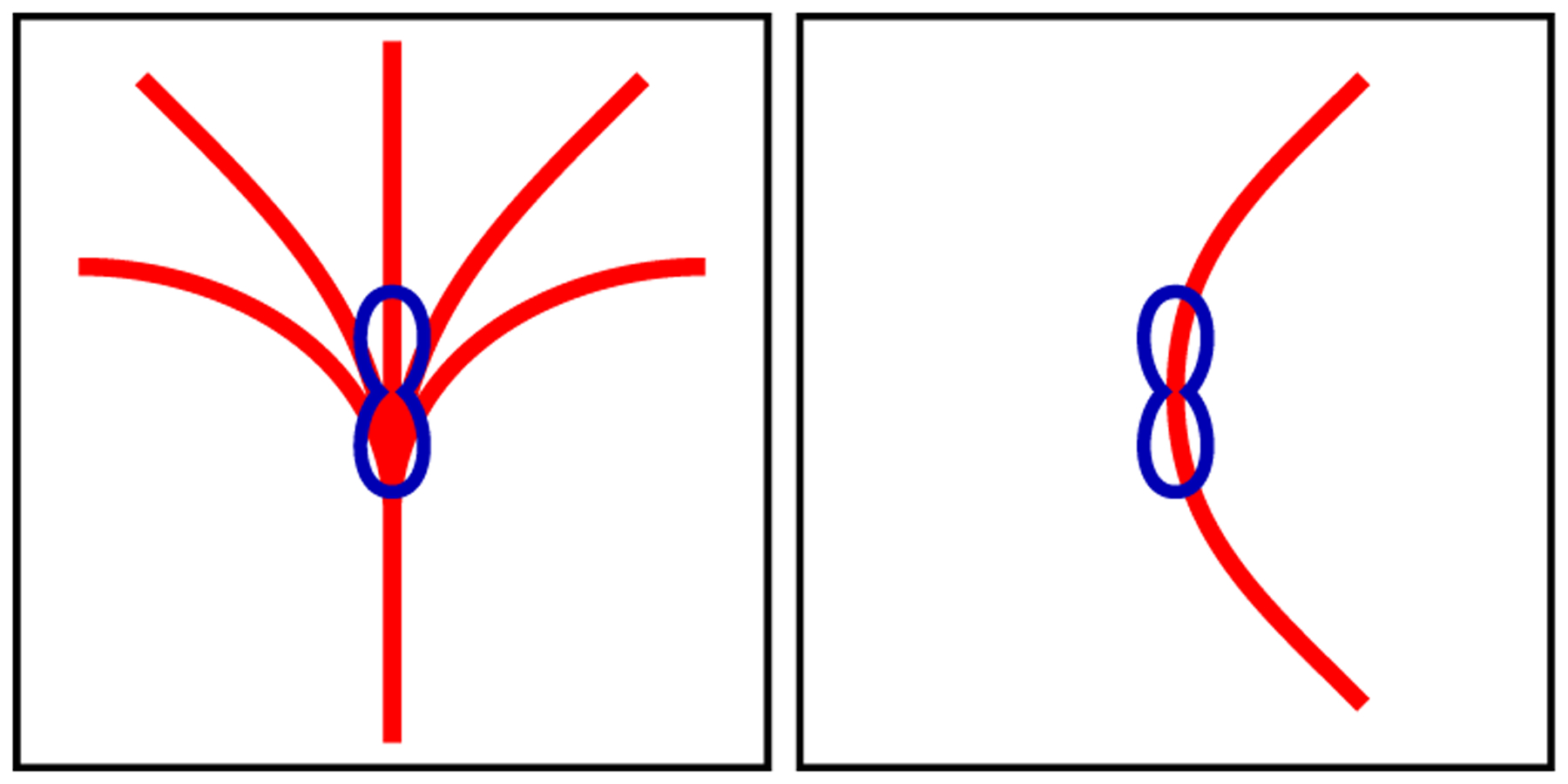
Solving these parameters is an ill-posed problem. For example, Fig. 1 illustrates that, due to the symmetrical nature of diffusion-weighted MR measurements, the resulting fiber orientation distribution functions (ODFs) are symmetric and do not distinguish between curving and fanning fiber configurations. Put differently, even though the fiber segments that form the fibers traversing this voxel are located and oriented in radically different configurations, the signal observed within this voxel cannot be used to disambiguate between the configurations, let alone be used to estimate the configurations of the fiber segments. One viable solution to this is to gather information from neighboring, anatomically connected voxels to regularize the problem. The continuous nature of the fiber trajectories provides subvoxel information that can help super-resolve the voxel. This provides a powerful mechanism that allows us to collapse measurements across multiple voxels to estimate micro-structural properties with spatial resolution that is finer than the voxel dimensions. We will show that the associated problem can be solved by using the Metropolis-Hastings algorithm [2, 5], a Markov chain Monte Carlo (MCMC) method that is well suited for solving high-dimensional problems.

Fig. 1. Ambiguity Due to Partial Volume Effect.

Radically different subvoxel fiber configurations (red) can result in similar fiber ODF shapes (blue).

2. Approach

We assume that the signal at each voxel is an agglomeration of signals from constituent fiber segments that reside within the voxel. Formally, denoting the signal at location x and gradient direction g as E(x, g) = S(x, g)/S₀(x), we define the generative model of this signal in the form of spatio-angular decomposition:

$$E(x,g)=\sum _{i}G\left(x,x_i\right)E_i(g)+\epsilon (x,g)\text{\hspace{1em}s.t.\hspace{1em}}\mathcal{M}.$$ (1)

Our task is to solve for the parameters of model $\mathcal{M}$ by minimizing error ε(x, g) and at the same time imposing some form of regularity on the solution, i.e,

$$\underset{\mathcal{M}}{\text{min}}[\Theta (\mathcal{M})]=\underset{\mathcal{M}}{\text{min}}\left\{\underset{{\Omega }_x\times {\Omega }_g}{\int }{|E(x,g)-\sum _{i}G\left(x,x_i\right)E_i(g)|}^{2}dxdg+\gamma \Phi (\mathcal{M})\right\}.$$ (2)

Here $G\left(x,x_i\right)=e^{-{|x-x_i|}^2/{\sigma }^2}$ models the smoothing effect owing to signal averaging and Φ(·) is a regularization term that enforces a certain degree of cross-voxel smoothness in the model $\mathcal{M}$, which encodes the fiber configuration. The predicted signal is generated via an ensemble of constituent signals {E_i(·)}, each assumed to be generated by the i-th fiber segment located at x_i. γ is a tuning parameter that balances the two terms. The L₂-norm is evaluated over all locations (denoted by set ${\Omega }_x\subset {ℝ}^3$) and gradient directions (denoted by set ${\Omega }_g={\mathbb{S}}^2$), i.e., the position-orientation space (POS). The goal here is to determine the parameters (i.e., locations and orientations) of the fiber segments that will result in a configuration that can best explain the observed signal E(x, g). Unlike approaches such as spherical deconvolution [10] that seek to decompose the signal at each voxel on the ${\mathbb{S}}^2$ domain; our framework seeks a ${ℝ}^3\times {\mathbb{S}}^2$ decomposition. The additional spatial component provides sub-voxel information that is important for resolution enhancement. Note that since we are in practice only concerned with white matter, the observed and predicted signals in (2) are first centralized by removing their means so that isotropic diffusion will not affect the outcome; a similar approach was used in [4, 7].

2.1. Signal Generating Fiber Segments

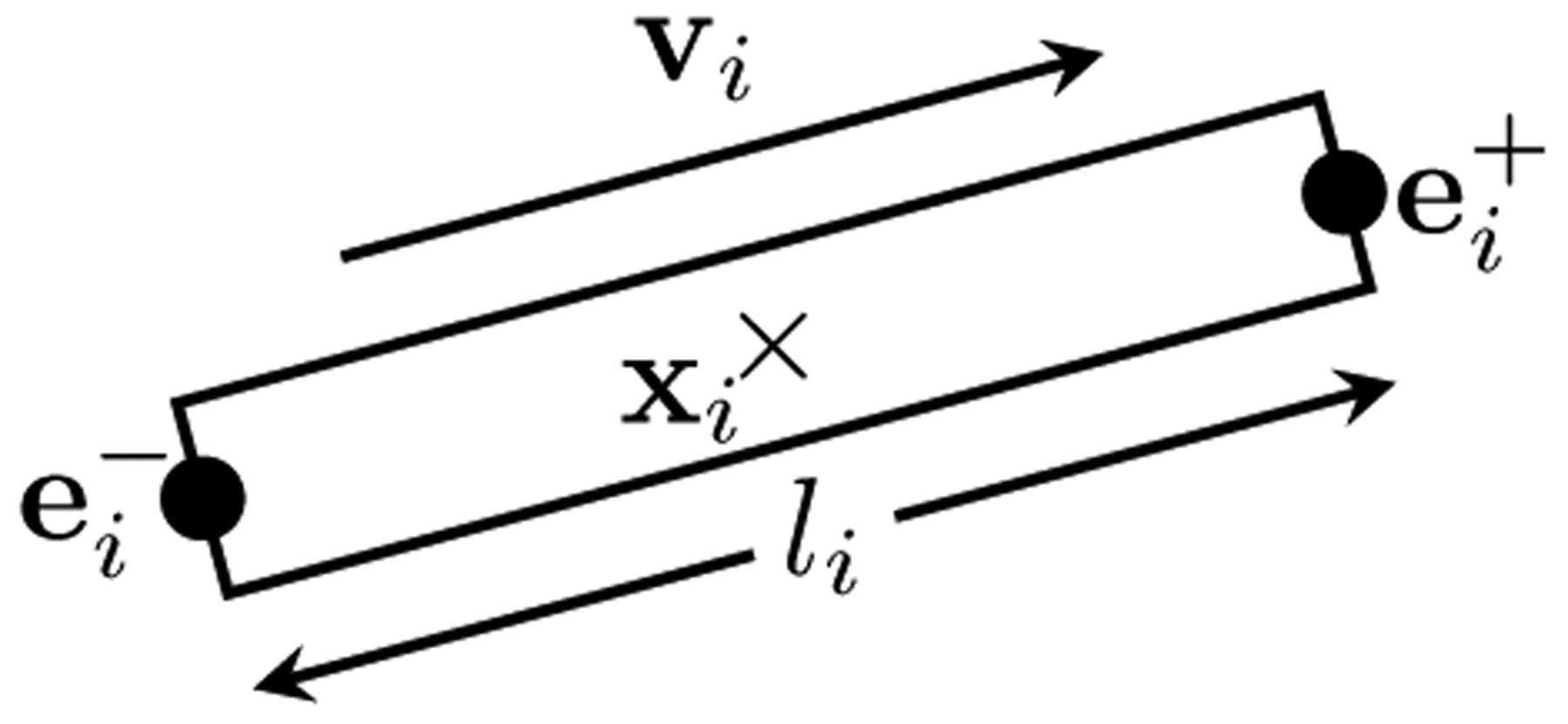
Our method assumes that an arbitrary number of fiber segments can reside within a voxel space. Each fiber segment is represented by a cylinder that contributes a signal typical of parallel fibers within the voxel it resides. Each cylinder (see Figure 2) is defined by the tuple h_i = (x_i, v_i, l_i, d_i). The three-dimensional vector x_i specifies the center of the cylinder, and v_i is a unit vector that defines its orientation. The length l_i and diameter d_i are predefined and are identical for all cylinders (i.e., l_i = l, d_i = d, ∀i). The two ends $e_i^{+}$ and $e_i^{-}$ of the cylinder h_i are determined by $e_i^{+}=x_i+\frac{l_i}{2}{v}_i$ and $e_i^{-}=x_i-\frac{l_i}{2}{v}_i$. The cylinders can be connected at the ends, e.g., $e_i^{+}=e_{i+1}^{-}$ and $e_i^{-}=e_{i-1}^{+}$. Each fiber segment i is assumed to generate signal based on a single-tensor model, i.e., $E_i(g)=w{e}^{-b{g}^{\text{T}}{\text{D}}_{i}g}$, where b is the diffusion weighting. $D_i={\lambda }_1{v}_i{v}_i^{\text{T}}+{\lambda }_{2}I$ denotes a diffusion tensor with diffusivities λ₁ and λ₂ and principal diffusion direction v_i, which is equivalent to the orientation of the fiber segment. Constant $w\in {ℝ}^{+}$ controls the amount of signal contribution from each fiber segment.

Fig. 2. A Fiber Segment.

The signal at each voxel is assumed to be an accumulation of signal generated by an ensemble of fiber segments.

2.2. Fiber Continuity as Regularization

The regularization term $\Phi (\mathcal{M})$ is important to ensure that the otherwise ill-posed minimization of $\Theta (\mathcal{M})$ in (2) is tractable. The model $\mathcal{M}$ here consists of a set of fiber segments $\mathcal{H}=\left\{h_i\right\}$ as well as their connections $\mathcal{E}=\left\{\left(e_i^{{\alpha }_i},e_j^{{\alpha }_j}\right)\right\}$ with α ∈ {+, −}. Smooth transition in both location and orientation is expected from fiber segments that are connected. Similar to [8], this is enforced by defining

$$\Phi (\mathcal{M})=\sum _{\left(e_i^{{\alpha }_i},e_j^{{\alpha }_j}\right)\in \mathcal{E}}\frac{1}{l^2}\left({\Vert e_i^{{\alpha }_i}-{\overline{x}}_{ij}\Vert }^2+{\Vert e_j^{{\alpha }_j}-{\overline{x}}_{ij}\Vert }^2\right)-L,$$ (3)

where ${\overline{x}}_{ij}=\frac{x_i+x_j}{2}$ is the midpoint of the line connecting the centers of the i-th and j-th fiber segments. Parameter L controls the likeliness of connections. A large L causes two segments to be connected with higher likeliness. The first two terms of the above equation encourages the fiber segments to be close to each other, but not closer than the length of the segments. The fiber segments are also encouraged to be aligned by penalizing the misalignment of v_i and v_j.

2.3. The Metropolis-Hastings Algorithm

We minimize $\Theta (\mathcal{M})$ in (2) by utilizing the Metropolis-Hastings algorithm [2, 5]. This is equivalent to maximizing the posterior distribution $P(\mathcal{M}|\mathcal{D})$. That is, we need to determine the most probable $\mathcal{M}$ given the observed data $\mathcal{D}$. The core idea of the Metropolis-Hastings algorithm is to update the model from $\mathcal{M}$ to ${\mathcal{M}}^{\prime }$ based on a proposal distribution $Q\left({\mathcal{M}}^{\prime }|\mathcal{M}\right)$ and accept the model update with probability min(1, R), where R is the so-called Green’s ratio

$$R={\left(\frac{P\left({\mathcal{M}}^{\prime }|\mathcal{D}\right)}{P(\mathcal{M}|\mathcal{D})}\right)}^{\frac{1}{T}}\frac{Q\left(\mathcal{M}|{\mathcal{M}}^{\prime }\right)}{Q\left({\mathcal{M}}^{\prime }|\mathcal{M}\right)}.$$ (4)

Temperature T is progressively lowered in a manner similar to simulated annealing so that the estimated posterior distribution can progressively become sharper and more defined. The algorithm works best if the proposal density $Q\left({\mathcal{M}}^{\prime }|\mathcal{M}\right)$ matches the shape of the target distribution $P\left({\mathcal{M}}^{\prime }|\mathcal{D}\right)$ from which direct sampling is difficult, that is $Q\left({\mathcal{M}}^{\prime }|\mathcal{M}\right)\approx P\left({\mathcal{M}}^{\prime }|\mathcal{D}\right)$. We follow the approach outlined in [8] to construct a proposal distribution. The model $\mathcal{M}$ is allowed to be modified by creation/deletion, connection/disconnection, and shifting of fiber segments. For more details, please refer to [8].

2.4. Generating High-Resolution Images

Once the optimal model ${\mathcal{M}}^{*}$ has been determined, high-resolution data can be sampled from the model using a grid with resolution (e.g., (1 mm)³) that is higher than the acquisition resolution. More formally, the sampled signal E′ (x, g) is obtained as

$$E^{\prime }(x,g)=\sum _i{G}^{\prime }\left(x,x_i\right)E_i(g)\text{\hspace{1em}s.t.\hspace{1em}}{\mathcal{M}}^{*},$$ (5)

where G′ (x, x_i) is the same function as G(x, x_i), but with the bandwidth σ reduced according to the up-sampling factor to reflect the reduced voxel size and the fact that the sampled signal should now come from a smaller neighborhood, in line with the actual MR acquisition mechanism. This in effect reduces the blurring effect associated with the larger voxel size and hence helps produce a super-resolved version of the data.

A scalar image indicating the anisotropy at each location can be generated with the help of (5). This can be achieved by considering the anisotropic energy of the fiber ODFs [10], i.e.,

$$A(x)={\int }_{{\Omega }_g}{E}^{\prime }(x,g)\otimes H(g)dg=\sum _i{G}^{\prime }\left(x,x_i\right){\int }_{{\Omega }_g}{E}_i(g)\otimes H(g)dg,$$ (6)

where ⊗ denotes the spherical deconvolution operator, and H(g) is the responseT function of a directionally coherent fiber bundle. If we let $H(g)=w{e}^{-b{g}^{\text{T}}Dg}$, where D = λ₁vv^T+λ₂I with an arbitrary v, then (6) gives A(x) ∝ ∑_i G′ (x, x_i). Essentially, this implies that the anisotropic energy A(x) at each location x can be evaluated by a weighted count of fiber segments in the vicinity of x. On the surface, this approach resembles track-density imaging (TDI), as reported in [1]; however, in TDI no signal model is attached to the fiber segments and an arbitrarily huge or tiny number of fibers are allowed to transverse each voxel. This makes interpretation of the fiber count based image contrast generated by TDI very difficult.

3. Experimental Results

We report here preliminary results from our evaluation of the proposed technique using two different in vivo datasets, one acquired at the common (2 mm)³ resolution, the other at (1 mm)³ resolution.

3.1. Materials

Diffusion-weighted images for an adult subject were acquired at the typical (2 mm)³ resolution using a Siemens 3T TIM Trio MR scanner. Diffusion gradients were applied in 120 non-collinear directions with diffusion weighting b = 2,000s/mm². An additional set of high-resolution (1 mm)³ diffusion-weighted images were acquired from a different adult subject using the same scanner with the acquisition technique reported in [6]. Diffusion gradients were applied in 42 non-collinear directions with diffusion weighting b = 1,000s/mm².

3.2. Parameters

Setting the parameters of our algorithm to the following values was found to yield reasonable results. Regularization tuning parameter: γ = 1; tensor model parameters: bλ₁ = 1, bλ₂ = 0; the weight of each fiber segment: w = 0.0018; the smoothing bandwidth: σ = d = 1 mm; the length of each fiber segment: l = 3 mm; the connection likelihood parameter: L = 10; and the initial temperature: T = 0.1, which was decreased to the final temperature T = 0.001 in 5 × 10⁷ iterations. More details on how to set these parameters can be found in [7, 8].

3.3. Results

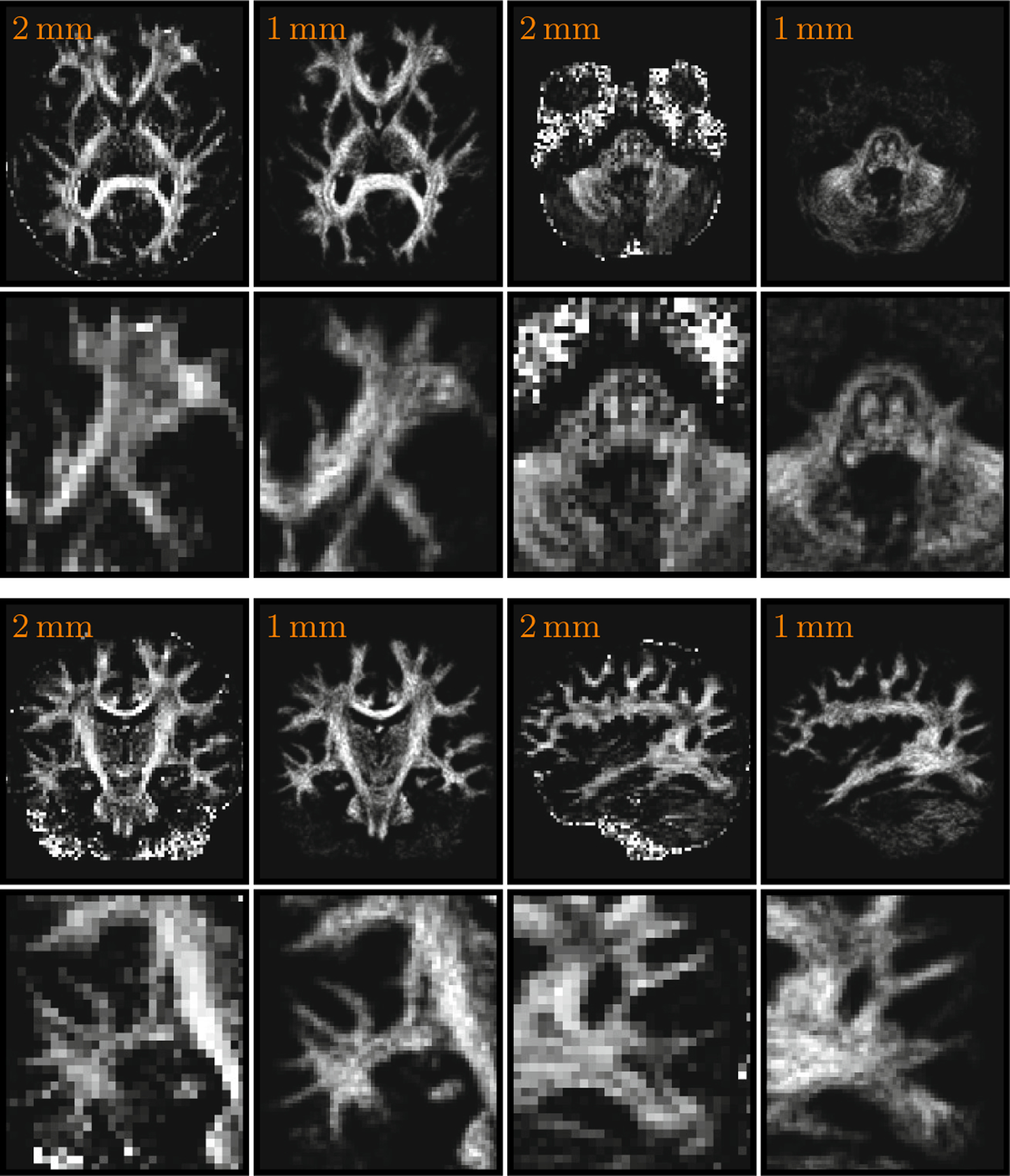
For preliminary evaluation, we applied our technique to the (2 mm)³ data and enhanced the resolution to (1 mm)³.The results, shown in Fig. 3, indicate that structural visibility can be significantly improved by using the proposed technique. Structures not visible in the low resolution becomes visible after enhancement.

Fig. 3. Results for (2 mm)³ Data.

Using our technique, the (2 mm)³ data are enhanced to (1 mm)³. The fractional anisotropy images are shown for the original data; the anisotropic energy images are shown for the enhanced data. The images in the second and fourth rows are closeup views of the images in first and third rows, respectively.

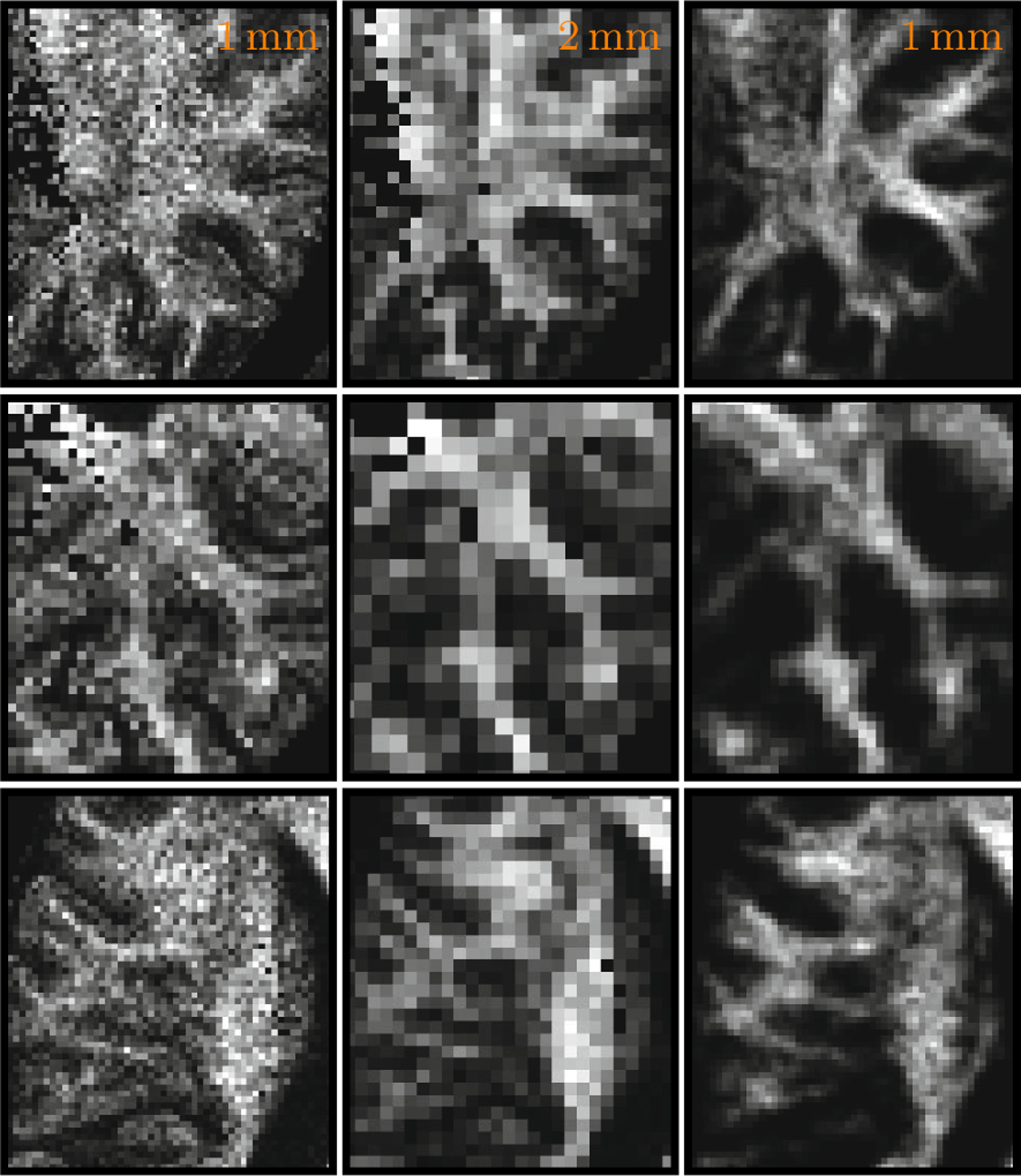
For better evaluation of the proposed technique, we down-sampled the (1 mm)³ data by averaging every 8 adjacent voxels to simulate a (2 mm)³ version of the data. This simulated low-resolution data were then enhanced using our technique to become (1 mm)³. The results, shown in Fig. 4, indicate that the resolution enhanced data retains most of the structures in the original high-resolution data. It can also be observed that the enhanced data are generally less noisy.

Fig. 4. Results for Simulated (2 mm)³ Data.

The high resolution (1 mm)³ data (left) were down-sampled by averaging every 8 adjacent voxels to simulate the (2mm)³ data (middle), which were then enhanced to the resolution of (1 mm)³ (right) by using our technique.

4. Conclusion

We have presented a method to learn a generative model for producing high-resolution DMRI data. The model consists of a set of fiber segments that are configured in a way that best explains the observed data. The high-resolution data are generated by sampling from this learned model using a grid with resolution that is higher than the acquisition resolution. Even though the results reported were preliminary, they do demonstrate that the proposed method is effective and produces reasonable results.

References

- 1.Calamante F, Tournier J, Jackson G, Connelly A: Track-density imaging(TDI): Super-resolution white matter imaging using whole-brain track-density mapping. Neuroimage 53(4), 1233–1243 (2010) [DOI] [PubMed] [Google Scholar]
- 2.Hastings WK: Monte Carlo sampling methods using Markov chains and their applications. Biometrika 57(1), 97–109 (1970) [Google Scholar]
- 3.Johansen-Berg H, Behrens TE (eds.): Diffusion MRI — From Quantitative Measurement to In vivo Neuroanatomy. Elsevier; (2009) [Google Scholar]
- 4.Kreher B, Mader I, Kiselev V: Gibbs tracking: A novel approach for the reconstruction of neuronal pathways. Magnetic Resonance in Medicine 60(4), 953–963 (2008) [DOI] [PubMed] [Google Scholar]
- 5.Metropolis N, Rosenbluth A, Rosenbluth M, Teller A, Teller E: Equations of state calculations by fast computing machines. Journal of Chemical Physics 21(6), 1087–1092 (1953) [Google Scholar]
- 6.Porter DA, Heidemann RM: High resolution diffusion-weighted imaging using readout-segmented echo-planar imaging, parallel imaging and a two-dimensional navigator-based reacquisition. Magnetic Resonance in Medicine 62(2), 468–475 (2009) [DOI] [PubMed] [Google Scholar]
- 7.Reisert M, Mader I, Anastasopoulos C, Weigel M, Schnell S, Kiselev V: Global fiber reconstruction becomes practical. NeuroImage 54(2), 955–962 (2011) [DOI] [PubMed] [Google Scholar]
- 8.Reisert M, Mader I, Kiselev V: Global reconstruction of neuronal fibres. In: Medical Image Computing and Computer Assisted Intervention (MICCAI), Diffusion Modelling Workshop (2009) [Google Scholar]
- 9.Scherrer B, Gholipour A, Warfield S: Super-resolution reconstruction to increase the spatial resolution of diffusion weighted images from orthogonal anisotropic acquisitions. Medical Image Analysis 16(7), 1465–1476 (2012) [DOI] [PMC free article] [PubMed] [Google Scholar]
- 10.Tournier JD, Calamante F, Gadian DG, Connelly A: Direct estimation of the fiber orientation density function from diffusion-weighted MRI data using spherical deconvolution. NeuroImage 23(3), 1176–1185 (2004) [DOI] [PubMed] [Google Scholar]
- 11.Yap P-T, Shen D: Resolution enhancement of diffusion-weighted images by local fiber profiling. In: Ayache N, Delingette H, Golland P, Mori K (eds.) MICCAI 2012, Part III. LNCS, vol. 7512, pp. 18–25. Springer, Heidelberg: (2012) [DOI] [PMC free article] [PubMed] [Google Scholar]