Quantifying the Bias due to Observed Individual Confounders in Causal Treatment Effect Estimates

Abstract

It is often of interest to use observational data to estimate the causal effect of a target exposure or treatment on an outcome. When estimating the treatment effect, it is essential to appropriately adjust for selection bias due to observed confounders using, for example, propensity score weighting. Selection bias due to confounders occurs when individuals who are treated are substantially different from those who are untreated with respect to covariates that are also associated with the outcome. A comparison of the unadjusted, naive treatment effect estimate with the propensity score adjusted treatment effect estimate provides an estimate of the selection bias due to these observed confounders. In this paper, we propose methods to identify the observed covariate that explains the largest proportion of the estimated selection bias. Identification of the most influential observed covariate or covariates is important in resource-sensitive settings where the number of covariates obtained from individuals needs to be minimized due to cost and/or patient burden and in settings where this covariate can provide actionable information to healthcare agencies, providers, and stakeholders. We propose straightforward parametric and nonparametric procedures to examine the role of observed covariates and quantify the proportion of the observed selection bias explained by each covariate. We demonstrate good finite sample performance of our proposed estimates using a simulation study and use our procedures to identify the most influential covariates that explain the observed selection bias in estimating the causal effect of alcohol use on progression of Huntington’s disease (HD), a rare neurological disease.

1 |. INTRODUCTION

It is often of interest to use observational data to estimate the causal effect of a target exposure or treatment on an outcome. However, given the nature of observational data (e.g, that researchers cannot control the assignment of individuals or units to levels of the target exposure or treatment), methods are needed to ensure groups being compared are well-balanced with respect to all potential pre-treatment (or pre-exposure) confounders. In the absence of balanced groups, it is likely that the estimated effect of the exposure or treatment will be biased.^1,2,3 This bias is often referred to as “selection bias” because it results from individuals or units “selecting” to receive certain exposures or treatments, although for many applications this is not necessarily a reflection of individual choice. Propensity scores are frequently used in practice to reduce or eliminate selection bias due to the observed confounders available in a data set by obtaining better comparability between the groups of interest, at least in terms of the observed covariates used in the propensity score model.^4,5,6 If all known pre-treatment confounders are included in the propensity score model, then a treatment effect estimate that adjusts for the propensity score has the potential ability to remove selection bias completely from the estimated treatment effect.^4,7,8

In most practical applications using propensity score adjustment, it is useful to examine how much the treatment effect estimate has shifted pre- versus post- propensity score adjustment to understand the influence of selection bias due to observed confounders in a study. The shift or difference between the naive treatment effect estimate and the propensity score adjusted treatment effect estimate provides an estimate of the selection bias that is due to the observed covariates. Quantifying the magnitude of this bias can be useful for understanding the impact that propensity score adjustment has on the estimated treatment effect. In some settings, researchers seek to understand how much of the selection bias due to observed confounders (e.g., referred to here as “observed selection bias”) is explained by a single confounder of interest or by a subset of confounders, particularly when identification of an important confounder can provide actionable information for agencies and stakeholders. For example, in health disparities studies comparing health outcomes between Hispanics and non-Hispanic Whites, estimation of the racial difference in health outcomes can be made more robust by using propensity score adjustment to balance Hispanics and non-Hispanics on observed potential confounders and, in the process, may identify specific variables (e.g., insurance status and receipt of preventative care early in life) as important observed confounders that explain the observed differences in health outcomes for these two populations.^9,10,11 Thus, adjustment for the observed selection bias due to these factors is critical when trying to estimate the size of racial disparities on health outcomes. Additionally, understanding what percentage of the observed selection bias is explained by a particular confounder or set of confounders may also provide actionable information for policymakers as it points to a need to further investigate the causes for the differences (e.g., in our example, the differences in insurance status and use of preventative care early in life may be a potential reflection of disparities within the healthcare system).^12,13,14 While race/ethnicity is not modifiable in the classic sense of an intervention or treatment (and thus causal effects cannot be estimated), propensity score methods and other causal inference methods can be utilized to ensure more robust estimation of health disparities that are an urgent and relevant public health concern.

Even if a particular confounder is not actionable, measurement cost or burden may also motivate researchers to understand how much influence a specific observed variable has on the shift in the estimated treatment effect. For example, in health care studies of chronic or terminal disease, there are often potential confounders that are costly, burdensome, or invasive to measure or obtain. In those settings, it is important to understand whether that covariate can be removed from the adjustment while still ensuring unbiased treatment effect estimation to efficiently utilize resources and not cause undue burden to patients. Additionally, in studies with smaller sample sizes like our application which focuses on a rare disease, it is often of interest to minimize the total number of variables being used in the propensity score model to avoid overfitting. However, in both of these cases, it is critical to robust inferences that research not discard true confounders. We aim to create methods that can quantify the proportion of the observed selection bias that is explained by each individual observed confounder in a study, such that this quantity can inform policy-related decisions and such that only necessary observed confounders can be used to estimate an unbiased treatment effect in a resource-sensitive setting.

While many studies of health outcomes and disparities would benefit from a better understanding of how much each observed confounder contributes to the shift in treatment effect estimates pre- and post- propensity score adjustment (i.e, the observed selection bias or selection bias due to observed confounders), there are no readily available methods to quantify the role of each observed covariate in explaining the observed selection bias. This paper aims to develop useful methods and tools for implementing such analyses. We propose two different ways to explore the problem. In the first, we develop quantities that can be used to understand the individual impact of each observed confounder by investigating how much the treatment effect would change if a study only controlled for one covariate. In the second, we develop quantities that can be used to understand the individual impact of each observed confounder when it is removed from the fully adjusted treatment effect estimate, thereby providing an understanding of its added value above and beyond all the other observed confounders used in the propensity score model.

In Section 2, we present notation, discuss assumptions, and describe our proposed methods. In Section 3, we present methods for estimating the relative impact of each observed confounder on explaining the observed selection bias in an analysis; we also discuss parametric and nonparametric methods for estimating the needed propensity score weights and the implications of balance assessment. In Section 4, we use a simulation study to demonstrate that our proposed methods perform well across a variety of settings. In Section 5, we apply our methods to observational data to examine the impact of alcohol use on Huntington’s disease (HD), a rare neurological disease.

2 |. NOTATION, DEFINITIONS, AND PROPOSED QUANTITIES

2.1 |. Notation and Definitions

Let $Y_i^{obs}$ denote the observed outcome of interest for individual i, T_i denote the binary treatment or intervention, where T_i = 0 or 1, and X_i = {X_1i, X_2i, …, X_ki} denotes the vector of available baseline/pre-treatment covariates. For example, in our HD application, Y is the severity level of the disease ranging in values from −3 to 3 with a standard deviation of 1 and such that higher values indicate greater severity of the disease; T is whether or not someone is an alcohol drinker at study initiation; and X_i includes the key confounders of interest including the CAG repeats an individual has (measured via blood work and for which higher values typically mean earlier onset and worse symptoms of the disease), the baseline severity of the patient at intake, age, education level, drug use, and antidepressant use.^15,16,17 In the case of binary treatments or exposures, each individual has two potential outcomes: the Y_i that would be observed if the individual was assigned to treatment group 1 and the Y_i that would be observed if the individual was assigned to treatment group 0, only one of which is observable for each individual. Let Y_1i and Y_0i denote the potential outcomes when T_i = 1 and T_i = 0, respectively. Then, $Y_i^{obs}=Y_{1i}$ if T_i = 1 and Y_0i if T_i = 0.

Using this notation, we want to estimate the average treatment effect on the population (ATE), denoted as Δ:

$$\Delta =E\left(Y_{1i}-Y_{0i}\right)=E\left(Y_{1i}\right)-E\left(Y_{0i}\right).$$

Let ${\widehat{\Delta }}^{\mathit{\text{naive}}}$ be the naive estimator of Δ where we simply take the difference in means between the two treatment groups (here, alcohol drinkers minus non-drinkers),

$${\widehat{\Delta }}^{\mathit{\text{naive}}}=\frac{1}{n_1}\sum _{i:T_i=1}{Y}_i^{obs}-\frac{1}{n_0}\sum _{i:T_i=0}{Y}_i^{obs}.$$

We know that if there is selection bias¹⁸ due to observed and unobserved confounders, this estimate will be a biased estimate of Δ. Since treatment is not randomized, we have to account for the pre-treatment differences between those with T_i = 0 and T_i = 1. If we assume that

$$T_i\perp Y_{1i},Y_{0i}\mid X_i,$$ (A1)

(e.g., the treatment is strongly ignorable (or has unconfoundedness) with respect to X_i and thus, there are no unobserved confounders) then we can estimate Δ through propensity score weighting where p_i = P(T_i = 1|X_i) and

$${\widehat{\Delta }}^{ps}=\frac{{\sum }_{i:T_i=1}{Y}_i^{obs}{W}_i}{{\sum }_{i:T_i=1}{W}_i}-\frac{{\sum }_{i:T_i=0}{Y}_i^{obs}{W}_i}{{\sum }_{i:T_i=0}{W}_i}$$

where

$$W_i=\left\{\begin{array}{ll}1/p_i\hfill & \text{ if }{T}_i=1\hfill \\ 1/\left(1-p_i\right)\hfill & \text{ if }{T}_i=0\hfill \end{array}\right.$$

Now let

$$\widehat{\lambda }={\widehat{\Delta }}^{\mathit{\text{naive}}}-{\widehat{\Delta }}^{ps}$$

such that $\widehat{\lambda }$ is an estimate of the the selection bias attributable to this set of observed confounders (referred to here as the observed selection bias), X_i. Importantly, the estimated $\widehat{\lambda }$ Will only be an estimate of the selection bias and may in truth reflect a combination of both selection bias and model misspecification, depending on the use of any models to estimate ${\widehat{\Delta }}^{ps}$. If there is no selection bias due to the observed confounders used in our analysis (and no unobserved confounders), then λ = 0. However, in most practical applications selection bias due to observed confounders will exist and thus, λ ≠ 0. If both treatment effect estimates are in the same direction, then $\widehat{\lambda }>0$ implies that the naive treatment effect underestimates the true treatment effect and $\widehat{\lambda }<0$ implies that it overestimates the true treatment effect. Thus, $\widehat{\lambda }$ provides us with an estimate of the selection bias attributable to the observed pre-treatment confounders included in the propensity score model. Our aim is to determine how much of the observed selection bias is explained by each observed confounder included in X_i. Thus, for our HD example, it is of interest to understand how much of the observed selection bias in the naive estimate of alcohol’s impact on HD severity is driven by each observed confounder included in X_i (i.e., CAG repeats, baseline HD severity, age, education, drug use, and antidepressant use). In Sections 2.3 and 2.4, we present two straightforward ways to quantify the amount of the observed selection bias accounted for by each observed confounder.

2.2 |. Assumptions

There are four common assumptions that are required for robust inference when utilizing propensity scores to estimate treatment effects: consistency, unconfoundedness, positivity, and no interference. Consistency requires that a subject’s potential outcome under the treatment received (here, their observed treatment) equals the subject’s observed outcome. Unconfoundesness (or strong ignorability)¹⁹ requires that there are no unobserved confounders that have not been included in the covariates used to estimate weights and is equivalent to (A1) defined earlier. Thus, assumption (A1) assumes that all confounders are captured in X and that therefore, there are no unmeasured confounders. Positivity assumes that each individual has a positive probability of receiving the treatment i.e., that no individual (in the analysis) has probability equal to 1 or 0 of receiving the treatment/being in the treatment group. This is also commonly referred to as having overlap or positivity between the treatment and control groups on all pre-treatment confounders and can be written as

$$0<p_i<1\forall i.$$ (A2)

Finally, no interference assumes that outcomes for individuals are not dependent on one another. Under these assumptions, ${\widehat{\Delta }}^{ps}$ will be a consistent estimate of Δ.⁴

2.3 |. Single confounder removal

In our first approach, referred to here as our single confounder removal approach, the goal is to estimate the bias that would result in the adjusted treatment effect if one were to remove the confounder of interest (in essence assuming that the full adjusted estimate is unbiased). Thus, in the HD example, we wish to understand the impact on the propensity score weighted effect estimate for alcohol use on HD severity if one excludes key confounders such as CAG from their analysis. A priori, one would expect removal of CAG to have a big impact due to the fact that it is one of the strongest available predictors of HD disease onset and progression.²⁰ We define this adjusted treatment effect that excludes the confounder X_j as:

$${\widehat{\Delta }}^{ps}\left(-X_j\right)=\frac{{\sum }_{i:T_i=1}{Y}_i^{obs}{W}_i\left(-X_j\right)}{{\sum }_{i:T_i=1}{W}_i\left(-X_j\right)}-\frac{{\sum }_{i:T_i=0}{Y}_i^{obs}{W}_i\left(-X_j\right)}{{\sum }_{i:T_i=0}{W}_i\left(-X_j\right)}$$

where p_i(−X_j) = P(T_i = 1|X_i\{X_ji}), X_i\{X_ji} denotes the vector X_i with the element X_ji removed, and

$$W_i\left(-X_j\right)=\left\{\begin{array}{ll}1/p_i\left(-X_j\right)\hfill & \text{ if }{T}_i=1\hfill \\ 1/\left(1-p_i\left(-X_j\right)\right)\hfill & \text{ if }{T}_i=0.\hfill \end{array}\right.$$

We then define

$$\widehat{\lambda }\left(-X_j\right)={\widehat{\Delta }}^{ps}-{\widehat{\Delta }}^{ps}\left(-X_j\right)$$

such that $\widehat{\lambda }\left(-X_j\right)$ estimates the shift captured by the removed confounder X_j away from the fully adjusted treatment effect estimate. Therefore, the proportion of the observed selection bias explained by the removed confounder X_j can be represented by

$$R\left(-X_j\right)=\frac{\widehat{\lambda }\left(-X_j\right)}{\widehat{\lambda }}.$$

Unfortunately, this approach would only be useful if the bias explained by each confounder is additive, independent, and in the same direction. An alternative way to summarize the proportion explained so that it can accommodate more complex situations would be to define the total bias due to removal of the included observed covariates, β^R as

$${\beta }^R=\sum _{j=1}^k\left|\widehat{\lambda }\left(-X_j\right)\right|$$

and the proportion of the observed selection bias explained by confounder X_j as

$$\widehat{B}\left(-X_j\right)=\frac{\left|\widehat{\lambda }\left(-X_j\right)\right|}{{\beta }^R}.$$

Certainly, it will not necessarily be the case that β^R will be equal to $\widehat{\lambda }$, but is used as a tool to understand the contribution of each confounder to the estimated selection bias. This notation can easily be extended to handle the removal of more than one confounder, if desired. For example, one can define and estimate ${\widehat{\Delta }}^{ps}\left(-\left\{X_j,X_m,X_n\right\}\right)$ to examine the bias captured by the removed confounders X_j, X_m, X_n.

2.4 |. Single confounder inclusion

In our second approach, referred to as single confounder inclusion, we aim to estimate the bias removed from the naive treatment effect if one were to use a propensity score weighted treatment effect that only adjusted for a single observed pre-treatment covariate (e.g, say CAG repeats for HD). In this case, we define the propensity score weighted treatment effect that only adjusts for one covariate at a time as follows:

$${\widehat{\Delta }}^{ps}\left(X_j\right)=\frac{{\sum }_{i:T_i=1}{Y}_i^{obs}{W}_i\left(X_j\right)}{{\sum }_{i:T_i=1}{W}_i\left(X_j\right)}-\frac{{\sum }_{i:T_i=0}{Y}_i^{obs}{W}_i\left(X_j\right)}{{\sum }_{i:T_i=0}{W}_i\left(X_j\right)}$$

where p_i(X_j) = P(T_i = 1|X_ji)

$$W_i\left(X_j\right)=\left\{\begin{array}{ll}1/p_i\left(X_j\right)\hfill & \text{ if }{T}_i=1\hfill \\ 1/\left(1-p_i\left(X_j\right)\right)\hfill & \text{ if }{T}_i=0.\hfill \end{array}\right.$$

We then define

$$\widehat{\lambda }\left(X_j\right)={\widehat{\Delta }}^{\mathit{\text{naive}}}-{\widehat{\Delta }}^{ps}\left(X_j\right)$$

such that $\widehat{\lambda }\left(X_j\right)$ estimates the shift in the naive estimate captured by the observed confounder X_j. Similar to the above, we define the total bias due to inclusion of a single observed covariate, β^I as

$${\beta }^I=\sum _{j=1}^k\left|\widehat{\lambda }\left(X_j\right)\right|$$

and the proportion of this total bias explained by confounder X_j as

$$\widehat{B}\left(X_j\right)=\frac{\left|\widehat{\lambda }\left(X_j\right)\right|}{{\beta }^I}.$$

2.5 |. Choosing an approach

These two proposed approaches lead to different measures that quantify the influence of a particular variable, except in the case where all observed variables included in the propensity score model are independent and have an additive effect, which is not likely in practice. The selected approach will often depend on the substantive question of interest. If one is interested in a variable that is costly or invasive to measure, the confounder removal approach is likely preferred since the substantive question is whether a treatment effect can be robustly estimated without use of this variable so that future studies can avoid obtaining the measurement. If one is interested in identifying a variable that may be actionable i.e., to inform policy-relevant decisions, then the confounder inclusion approach is likely preferred. Here, the substantive question is - does this variable explain a substantial proportion of the observed selection bias? In our numerical studies we illustrate and discuss the different results obtained by these two approaches.

3 |. ESTIMATION

3.1 |. Estimation of Proposed Quantities

To estimate $\widehat{\lambda }\left(-X_j\right)$, $\widehat{\lambda }\left(X_j\right)$, $\widehat{B}\left(-X_j\right)$ and $\widehat{B}\left(X_j\right)$, one may consider a variety of approaches to estimate the propensity score weights. Here, we describe a nonparamatric approach and a parametric approach to estimate the needed propensity score weights for each of our ${\widehat{\Delta }}^{ps}\left(X_j\right)$, ${\widehat{\Delta }}^{ps}\left(-X_j\right)$, and ${\widehat{\Delta }}^{ps}$ quantities.

Considering a nonparametric approach, we propose using a kernel density estimator when p_i is to be estimated with only a single confounder, and a generalized boosted model (GBM) when p_i is to be estimated using more than one confounder. Specifically, when p_i is to be estimated with only a single continuous confounder, X_j, we propose to use the Nadaraya-Watson estimator of the conditional mean,²¹

$${\tilde{p}}_i\left(X_j\right)=\frac{{\sum }_{l=1}^n{K}_h\left(X_{lj}-X_{ij}\right)T_l}{{\sum }_{l=1}^n{K}_h\left(X_{lj}-X_{ij}\right)}$$

where K(·) is a smooth symmetric density function with finite support, K_h(·) = K(·/h)/h and h is a specified bandwidth. In our numerical examples, we use a normal density for K(·) and use the rule-of-thumb suggested by Scott²² for the bandwidth h such that h = 1.06 min(σ, IQR/1.34) * n⁻² where σ and IQR are the standard deviation and interquartile range of X_j, respectively. This estimate, ${\tilde{p}}_i\left(X_j\right)$ can then be used to obtain all subsequent quantities. When the confounder X_j is discrete, one can simply estimate p_i(X_j) as the average T_i within each category of X_j.

When p_i is to be estimated with more than one confounder, we propose to use GBM which is a nonparametric approach to model outcomes (binary, discrete, or continuous) that allows for interactions among covariates and flexible functional forms for the regression surface.²³ GBM approximates the regression surface through a piecewise constant model, in which the regression surface is constant over regions of the covariate space. The fitting algorithm involves partitioning the covariate space and assigning values to constant functions in the selected regions. Model building is automated through an iterative algorithm that adds terms to maximize the likelihood conditional on the model chosen through the previous iterations. GBM has been shown to have less bias than traditional regression approaches due to how it adaptively captures the functional form of the relationship between the covariates and treatment.^24,6,25 For more details on GBM for propensity score estimation, see McCaffrey et al.⁶ and Burgette et al..²⁶ We implement GBM here using the twang package in R to obtain ${\tilde{p}}_i\left(\left\{X_j,X_m\dots ,X_n\right\}\right)$ which estimates p_i({X_j, X_m…, X_n}) = P(T_i = 1|{X_ij, X_im…, X_in}) where {X_ij, X_im…, X_in} is any subset of X_i with size greater than 1.²⁷

Such a nonparametric approach can be an attractive choice because it allows us to avoid any reliance on correct model specification, though this comes at a cost if we are in a setting in which a parametric model is correctly specificied and it can be used to estimate the quantities of interest. A straightforward parametric estimation approach to estimate our quantities would be to use simple logistic regressions to estimate all propensity scores p_i, p_i(−X_j) and p_i(X_j). That is, to estimate p_i, we assume that the specified logistic model holds and use the resulting predicted probability that Y_i = 1 as an estimate, ${\widehat{p}}_i$, of p_i. A similar process can be used to obtain estimates of p_i(−X_j) and p_i(X_j), denoted as ${\widehat{p}}_i\left(-X_j\right)$ and ${\widehat{p}}_i\left(X_j\right)$. It is also possible to expand the logistic model to include interaction and nonlinear terms, if desired. We recommend expanding the model on an as needed basis if balance after propensity score weighting is not optimal (see Section 3.3) in order to obtain better quality weights.

3.2 |. Asymptotic Properties and Variance Estimation

Under the assumptions stated in Section 2.2, and assuming the specified model used within the estimation approach (if using parametric estimation) is correct, ${\widehat{\Delta }}^{ps}$ is a consistent estimate of Δ.^28,29 However, the estimates, ${\widehat{\Delta }}^{ps}\left(-X_j\right)$ and ${\widehat{\Delta }}^{ps}\left(X_j\right)$, are in general not converging in probability to quantities that are themselves of interest and are in fact, erred versions of Δ. Under correct model specification (unless using nonparametric estimation) these estimates are consistent with respect to these erred values, and thus allow us to obtain consistent estimates of functions of these quantities, namely $\widehat{B}\left(-X_j\right)$ and $\widehat{B}\left(-X_j\right)$. Our use of the absolute value to create the denominator of $\widehat{B}\left(-X_j\right)$ and $\widehat{B}\left(-X_j\right)$, function which is, of course, not continuous at 0, makes the asymptotic distribution of these estimates nonstandard. Thus, to obtain variance estimates for $\widehat{B}\left(-X_j\right)$ and $\widehat{B}\left(-X_j\right)$ we use boostrapping³⁰ and show in our simulation study that the resulting estimates approximate the empirical variance very well.

3.3 |. Balance Assessment

A critical piece to all propensity score weighted analyses is to check the quality of the propensity score weights produced. One does this by checking the comparability (or balance) of the groups after applying the propensity score weights. Extensive details on balance assessment can be found elsewhere.^31,27 In general, it is recommended to assess balance over multiple criteria. For simplicity, we focus here on computing and reporting for each covariate used in the propensity score calculation, the differences between the treatment and control group in terms of the effect size (ES) difference. Thus, for the fully adjusted treatment effect estimate $\left({\widehat{\Delta }}^{ps}\right)$, one would compute and examine these ES differences for all covariates included in X_i. For single confounder removal, with estimated treatment effects ${\widehat{\Delta }}^{ps}\left(-X_j\right)$, one would compute ES differences for all covariates in X_i except for the removed covariate X_j since balance should not be expected on this removed confounder. For single confounder inclusion, with estimated treatment effects ${\widehat{\Delta }}^{ps}\left(X_j\right)$, one would only compute the ES difference for the single covariate, X_j. In our analyses, we consider propensity score weights to be adequate when the ES differences between the two groups are all less than 0.1.

4 |. SIMULATION STUDY

4.1 |. Simulation Goals

The goals of our simulation study were to assess (1) the performance of our proposed estimation procedures in terms of estimating the proportion of bias explained by individual confounders in various settings, (2) whether our proposed approaches can correctly identify the most and least important confounder(s) with respect to explaining selection bias, (3) whether the removal and inclusion approaches are equivalent when the covariates are additive and independent, (4) the impact of correlated confounders on substantive conclusions, and lastly, (5) the impact of a situation in which one does not start with an unbiased treatment effect estimate i.e., if ${\widehat{\Delta }}^{ps}$ is a biased estimate of Δ.

4.2 |. Simulation Setup

Our simulation study setup mirrors the setup used by Setodji et al. and others.^32,33,24 All simulations include 5 covariates, use a sample size of 2000, use bootstrapping to obtain standard error estimates, and summarize results over 1000 replications. In simulation setting 1, covariates X₁ and X₃ were generated from a standard normal distribution and then dichotomized using the mean as the threshold; covariates X₂, X₄, and X₅ were generated from a standard normal distribution. Treatment assignment T was generated such that T ~ Bernoulli(p) with p = 1/[1+exp{−f(X)}] where in setting 1: f(X) = 0.8X₁ + 0.25X₂ + 0.6X₃ + 0.4X₄ + 0.1X₅. The outcome Y was generated as

$$Y=-3.85+0.73X_1+0.36X_2+0.5X_3+0.2X_4+0.1X_5+\tau T$$

with τ = 0 i.e. there is no true treatment effect. Note that in this setting, the covariates are independent and additive in an effort to explore goal #3 described above.

In simulation setting 2, we purposefully aim to produce a setting in which there are two confounders moderately associated with treatment but very weakly associated with the outcome. In this setting, the five covariates and the treatment are generated as is described in setting 1, but the outcome is generated as

$$Y=-3.85+0.73X_1+0.01X_2+0.5X_3+0.01X_4+0.1X_5+\tau T$$

with τ = 0, such that X₂ and X₄ are weakly associated with the outcome.

In setting 3, we introduce correlation between covariates and a more complex relationship with the treatment: covariates X₁ and X₂ were generated from a standard normal distribution and then dichotomized using the mean as the threshold; covariate X₃ was generated from a standard normal distribution; covariate X₄ and X₅ were generated such that they were correlated with X₁ and X₂ (correlation = 0.2), respectively. Treatment assignment was generated as in setting 1 but with $f(X)=0.8X_1+0.25X_4+0.6X_2+0.4X_3^2+0.1X_5+0.3X_2{X}_4+0.2X_3{X}_4+0.4X_1{X}_2$. The outcome Y was generated as Y = −3.85 + 0.73X₁ + 0.36X₄ + 0.5X₂ + 0.2X₃ + 0.1X₅ + τT with τ = 0. Given the correlation between covariates, we expect our results to reflect the non-identifiability of B(X_j) and B(−X_j) in such a case, and we aim to examine the effect on resulting conclusions about the most important confounder.

In simulation setting 4, we purposefully aim to produce a setting in which there is an unmeasured confounder so that the fully adjusted treatment effect estimate is expected to be biased from the start. In this setting, the five covariates are generated as described in setting 1 but an additional covariate X₆ from a standard normal distribution is also generated. Treatment assignment was generated using f(X) = 0.8X₁ + 0.25X₂ + 0.6X₃ + 0.4X₄ + 0.1X₅ + 0.2X₆ and the outcome was generated as Y = −3.85 + 0.73X₁ + 0.36X₂ + 0.5X₃ + 0.2X₄ + 0.1X₅ + 0.2X₆ +τT. Covariate X₆ is assumed unmeasured and thus, not included in any propensity score models. The proportion of individuals in the treatment group in settings 1, 2, 3, and 4 is 0.65, 0.73, 0.65, and 0.65, respectively.

4.3 |. Simulation Results

Simulation results described here are from the parametric estimation approach; results from the nonparametric approach are provided in the Appendix. Simulation results using the single confounder removal approach are shown in Table 1 and the top panel of Figure 1. The “truth” for all quantities was calculated via a large sample estimate, using a sample size of 100,000. For all settings, the true treatment effect was 0, while the naive treatment effect ranged from 0.22–0.41 across settings (using the large sample truth). For all settings, variable 1 is correctly identified as the variable that explains the highest proportion of the selection bias, with estimates of B(−X_j) ranging from 0.36–0.61 across settings. In settings 1 and 2, the bias in our estimation approach is marginal, all less than 0.005, and confounders that explain a small proportion of the selection bias (e.g. 0.01–0.05) are correctly identified as the least important confounders. In settings 3 and 4, where we have purposefully created complexities in the data generation to examine the impact on estimation - setting 3 has correlation between variables and setting 4 has an unmeasured confounder which causes bias from the start - we see some bias as would be expected, but the bias is relatively small with 0.06 being the highest bias observed. In addition, for these two settings, even with this small amount of bias, the overall substantive conclusions would be correct i.e., that variable 1 explains the highest proportion of the selection bias. For all settings and all variables, the standard error estimates obtained using bootstrapping approximate the empirical standard errors well. Results for estimation of λ(X_j) and λ(−X_j) across all settings are provided in the Appendix.

TABLE 1.

Single Confounder Removal: simulation results for B(−X_j) using parametric estimation with n = 2000;

Variable	1	2	3	4	5
Setting 1
Truth	0.3610	0.2300	0.1880	0.1950	0.0260
Estimate	0.3640	0.2260	0.1870	0.1980	0.0250
Bias	−0.0030	0.0040	0.0000	−0.0030	0.0010
ESE	0.0360	0.0380	0.0290	0.0270	0.0130
ASE	0.0364	0.0381	0.0292	0.0265	0.0124
Setting 2
Truth	0.6090	0.0110	0.3170	0.0180	0.0460
Estimate	0.6100	0.0130	0.3140	0.0200	0.0420
Bias	−0.0020	−0.0030	0.0030	−0.0030	0.0040
ESE	0.0450	0.0100	0.0430	0.0140	0.0210
ASE	0.0463	0.0104	0.0430	0.0149	0.0194
Setting 3
Truth	0.3910	0.1920	0.0440	0.3010	0.0710
Estimate	0.4440	0.1810	0.0170	0.3300	0.0280
Bias	−0.0530	0.0110	0.0270	−0.0290	0.0440
ESE	0.0410	0.0320	0.0130	0.0430	0.0160
ASE	0.0420	0.0310	0.0141	0.0426	0.0152
Setting 4
Truth	0.3100	0.2150	0.1940	0.1970	0.0840
Estimate	0.3650	0.2270	0.1870	0.1960	0.0250
Bias	−0.0540	−0.0110	0.0060	0.0000	0.0590
ESE	0.0370	0.0390	0.0290	0.0270	0.0130
ASE	0.0370	0.0386	0.0297	0.0270	0.0127

ESE = empirical standard error (standard deviation of estimates across the 1,000 replications); ASE = average standard error (average of standard error estimates across the 1,000 replications obtained using bootstrapping)

FIGURE 1.

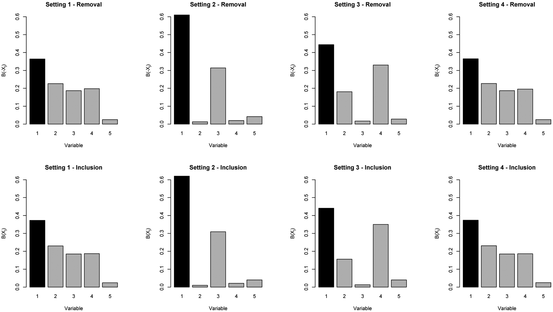
Illustrates the mean estimated B(−X_j) and B(X_j), across all variables in all settings using parametric estimation; shows Variable 1 is generally identified as the most influential variable using either approach

Simulation results using the single confounder inclusion approach are shown in Table 2 and the bottom panel of Figure 1. Similar to the single confounder removal approach, in all settings, variable 1 is correctly identified as the variable that explains the highest proportion of the selection bias, with estimates of B(−X_j) ranging from 0.37–0.62 across settings. In addition, confounders that explain a very small proportion of the selection bias, which change depending on the setting but generally have B(−X_j) values ranging from 0.01–0.04, are correctly identified as the least important confounders. For all settings and variables, the bias in our estimation approach is marginal, ranging from 0–0.01. Note that the correlation between variables in setting 3, and the unmeasured confounders in setting 4 do not have as large of an impact on bias using this approach compared to the single confounder removal. This is expected for setting 4, as the definition of B(X_j) does not rely on the fully adjusted estimate ${\widehat{\Delta }}^{ps}$.

TABLE 2.

Single Confounder Inclusion: simulation results for B(X_j) using parametric estimation with n = 2000;

Variable	1	2	3	4	5
Setting 1
Truth	0.3740	0.2360	0.1840	0.1840	0.0230
Estimate	0.3730	0.2300	0.1850	0.1870	0.0240
Bias	0.0000	0.0060	−0.0010	−0.0040	−0.0010
ESE	0.0400	0.0410	0.0310	0.0280	0.0140
ASE	0.0397	0.0408	0.0311	0.0281	0.0124
Setting 2
Truth	0.6240	0.0030	0.3120	0.0200	0.0410
Estimate	0.6200	0.0100	0.3090	0.0210	0.0400
Bias	0.0040	−0.0070	0.0040	−0.0010	0.0010
ESE	0.0490	0.0080	0.0470	0.0150	0.0220
ASE	0.0486	0.0101	0.0457	0.0165	0.0194
Setting 3
Truth	0.4510	0.1530	0.0100	0.3490	0.0360
Estimate	0.4410	0.1560	0.0130	0.3500	0.0400
Bias	0.0100	−0.0030	−0.0030	−0.0010	−0.0030
ESE	0.0340	0.0270	0.0100	0.0360	0.0150
ASE	0.0347	0.0259	0.0110	0.0356	0.0151
Setting 4
Truth	0.3780	0.2300	0.1870	0.1820	0.0240
Estimate	0.3740	0.2310	0.1850	0.1860	0.0250
Bias	0.0040	−0.0010	0.0020	−0.0040	−0.0010
ESE	0.0400	0.0410	0.0310	0.0280	0.0140
ASE	0.0403	0.0413	0.0315	0.0286	0.0126

ESE = empirical standard error (standard deviation of estimates across the 1,000 replications); ASE = average standard error (average of standard error estimates across the 1,000 replications obtained using bootstrapping)

Comparing the results and conclusions one would draw from the single confounder removal versus single confounder inclusion approach, these results show that in setting 1 where all variables are independent and additive, both approaches are essentially equivalent. Both suggest that the importance of the confounders as measured by the proportion of selection bias explained is X₁ (explains the most), X₂, X₃/X₄, and X₅ (explains the least). For settings 2–4, the numeric results differ depending on the approach but the results and conclusions are very similar as can be seen in Figure 1.

As is described in Section 3.3, the assessment of balance is always an important step when estimating a treatment effect using propensity scores. Figure 2 shows the average ES difference across all covariates in the propensity score model when all covariates are included (first boxplot) and when each covariate is removed, across the 1000 simulations in setting 1. This figure shows that balance is good using the initial full set of covariates, and we continue to have good balance even when a covariate is removed from the model.

FIGURE 2.

Assessing balance in setting 1 across 1,000 simulations: average absolute effect size among remaining variables using the single confounder removal approach

Results from the nonparametric approach are provided in the Appendix. Given the data generation, it is not unexpected that we would see more bias using the nonparametric estimation approach compared to when logistic regression is used. Generally, results and conclusions are similar, with variable 1 identified as most important and bias in estimates being relatively small ranging from 0.001 to 0.10 (setting 4). In addition, in the Appendix, we provide and discuss additional simulation settings and results with (a) smaller sample sizes of n = 500 and n = 1000, and (b) alternative settings including a setting where all regression coefficients are equal, a setting with a change in the prevalence of X₁, and settings with more complex generation schemes for the outcome and treatment.

5 |. HUNTINGTON’S DISEASE APPLICATION

Huntington’s disease (HD) is a rare genetically inherited neurological disorder, but it remains unclear how non-genetic factors such as environment and behavior contribute to its progression. Recent work by Griffin et al (under review) used propensity score weighting in a large (n=2,914) longitudinal dataset (Enroll-HD) to investigate the effects of non-genetic factors on HD progression. Notably, the study showed that there were meaningful shifts in the estimated effects of alcohol use on HD progression before and after propensity score weighting. This was due to the observed selection bias that resulted from the group differences between alcohol users and non-users at intake into the study. In particular, the non-users tended to have more severe HD at baseline than the alcohol users and had much later stages of HD. In the fully adjusted propensity score model, the study controlled for several important potential confounders (including CAG, intake HD severity, and age) to ensure that the groups were well balanced at baseline on observed confounders. However, the study did not explore the potential role of each observed confounder in explaining the shift in the estimated effect of alcohol. Here, we examine the role of each individual confounder in explaining the observed selection bias in the estimated effect of alcohol use on HD progression.

Given that HD is a rare disease, HD studies for new therapies or interventions often have small sample sizes and therefore it is of interest for HD researchers to understand covariates are most important to obtain and control for in estimating causal effects on HD progression. It is often not feasible for studies to obtain and control for all 19 confounders considered in the propensity score model from the Griffin et al (under review) study.^34,35,36,37

5.1 |. Data

Our analyses utilized data from Enroll-HD, a registry-based study of HD gene expansion carriers at over 160 clinical sites worldwide.²⁰ Enroll-HD provides a comprehensive repository of prospective data (demographics, medications, medical history, clinical features, family history and genetic characteristics) on a population of 16,000 participants. The dataset used here comes from the third version of Enroll-HD’s public use data set, released in December 2016, which merged together data for subjects who enrolled in both Enroll-HD and the former REGISTRY study.³⁸ Participants are assessed annually. We included adult individuals with the HD gene (e.g., those with CAG > 35 and age > 17 with late premanifest or stage 1 or 2 manifest HD at intake into the study).

The key exposure of interest was a binary indicator of any alcohol use as measured via self-reported units per week. The primary outcome was a previously developed composite outcome reflecting HD severity; the composite summarizes across seven common measures of HD severity that capture motor, functioning and cognition symptoms of HD. The composite ranges from approximately −3 to 3 and is normally distributed with a mean of 0 and a standard deviation of 1. Higher values of the composite indicate higher severity of the disease. The confounders used in this analysis include age, CAG, the outcome at baseline (e.g., baseline HD severity), education, drug use, and antidepressant use. Missingness of the data was low and handled via single imputation.

5.2 |. Results

Table 3 shows the baseline characteristics for our sample of alcohol using and non-using individuals on the observed confounders used in the propensity score model. Alcohol users tended to have lower mean CAG repeats (43.22 vs 43.68; ES difference = −0.14) and lower levels of baseline HD severity (−0.42 vs −0.04; effect size difference = −0.44) compared to non-users. They also had slightly higher rates of drug use, lower rates of antidepressant use, and higher levels of education.

TABLE 3.

Huntington’s Disease Application: Baseline Characteristics for Alcohol Users versus Non-Users;

	Alcohol Users	Non-Alcohol Users	ES Difference
Age, Years (Mean)	52.43	51.98	0.04
CAG repeats (Mean)	43.22	43.68	−0.14
Baseline HD Severity Level (Mean)	−0.42	−0.04	−0.44
Education (International Coding; %)
Primary	0.03	0.04	−0.08
Lower Secondary	0.19	0.23	−0.11
Upper Secondary/High School	0.26	0.33	−0.17
Post-secondary non-tertiary education	0.19	0.13	0.15
University Plus	0.33	0.26	0.15
Drug Use (%)	0.03	0.01	0.11
Antidepressant Use (%)	0.38	0.49	−0.22

CAG = cytosineadenine-guanine; and effect size (ES) <0.1 considered to denote small differences

Examining the effect of alcohol use on HD severity, the naive estimated impact of alcohol use on the HD composite outcome was ${\widehat{\Delta }}^{\mathit{\text{naive}}}=-0.46(p<0.001)$; the propensity score weighted estimate, using the nonparametric approach, was ${\widehat{\Delta }}^{ps}=-0.09(p=0.10)$. Thus, the estimated selection bias due to the observed covariates was $\widehat{\lambda }=-0.38$. This is a very large difference in the estimated treatment effect whereby the naive effect reflects a large protective effect of alcohol, but the fully adjusted effect estimate shows a null finding of no effect of alcohol use for HD severity after adjusting for the confounders.

Table 4 shows the results from our analysis, applying the proposed methods using nonparametric estimation. We use the nonparametric estimation approach in this example since it is highly unlikely that a simple logistic regression would be appropriate for this setting. First, let’s consider the single confounder inclusion results which allow us to directly assess the impact of adjusting for a single observed confounder on the naive treatment effect. As shown, the key confounder in this analysis that is driving the bias in the naive treatment effect is the baseline measure of HD severity. In the propensity score model that only includes this covariate, we obtain an adjusted ${\widehat{\Delta }}^{ps}\left(X_j\right)$ that equals −0.05, very different from the naive estimator $\left({\widehat{\Delta }}^{\mathit{\text{naive}}}=-0.46\right)$. Baseline HD severity explains 74% of the estimated selection bias using this approach. Examining the other confounders, both drug use and age contribute very little to shifting the bias in the naive treatment effect (< 1 %) while education, CAG, and antidepressant use shift the biased naive treatment effect only very marginally (5 − 11 %).

TABLE 4.

Huntington’s Disease Application: Results from Examining Individual Observed Confounders;

Single Confounder Inclusion
	Δps (Xj)	λ(Xj) [SE]	B(Xj) [SE]
Age	−0.47	0.01 [0.01]	0.01 [0.01]
CAG	−0.42	−0.04 [0.01]	0.08 [0.02]
Baseline HD Severity	−0.05	−0.41 [0.04]	0.74 [0.03]
Education	−0.40	−0.06 [0.01]	0.11 [0.02]
Drug Use	−0.46	0.00 [0.00]	0.00 [0.00]
Antidepressant use	−0.43	−0.03 [0.01]	0.05 [0.02]
Single Confounder Removal
	Δps (Xj)	λ(Xj) [SE]	B(Xj) [SE]
Age	−0.07	−0.02 [0.01]	0.08 [0.03]
CAG	−0.08	−0.01 [0.01]	0.04 [0.02]
Baseline HD Severity	−0.31	0.22 [0.03]	0.84 [0.04]
Education	−0.08	−0.01 [0.01]	0.03 [0.02]
Drug Use	−0.09	0.00 [0.00]	0.00 [0.01]
Antidepressant use	−0.09	0.00 [0.00]	0.01 [0.01]

SE = standard error

In terms of single confounder removal, we see a similar story, though now we are examining the impact of removing an observed covariate from the fully adjusted propensity score model. As shown, removing HD severity again has the greatest impact, whereby the differences in the fully adjusted propensity score weighted treatment effect and the propensity score weighted model that excludes baseline HD severity results in a total shift of $\widehat{\lambda }\left(-X_j\right)=0.22$. Using this approach, HD severity accounts for 84% of the estimated selection bias while all the other confounders each explain less than 8%.

As noted in Section 2, it is important to assess balance for each of the propensity score models used in our approach. In this application, the average ES difference calculated across all confounders included in the propensity score model was less than 0.10, for each examined model (confounder inclusion and removal).

The applied implications of these analyses are useful for the field of HD research as baseline severity or baseline measures of the outcome are often not controlled for in HD studies.^{36,37,39,40,41,42,43,44,45} The prior tradition in the field has been to control for age and CAG as the most important confounders of treatment and HD progression. It is clear from our analyses that controlling for HD severity at intake is critically important in order to reduce the selection bias in the estimated treatment/exposure effect.

6 |. DISCUSSION

We proposed two approaches to quantify the role of each observed covariate in explaining the estimated selection bias, a confounder inclusion approach and a confounder removal approach. These approaches lead to different measures that quantify the influence of a particular observed confounder in the analysis and the selected approach will often depend on the substantive question of interest. These methods are straightforward, intuitive, and easy to implement; code to implement these procedures is available in the R package SBdecomp available on Github at https://github.com/laylaparast/SBdecomp. Additionally, our HD application highlights an important applied finding for HD research whereby baseline severity of the disease proves to be the primary confounder driving the selection bias in our case study. This implies that controlling for baseline HD severity will likely remove the large majority of observed selection bias in effect estimates for non-genetic factors like alcohol use. This is notable for the field since analyses using observational studies often have overlooked the importance of balancing groups on baseline severity of the disease, traditionally assuming that age and CAG repeats together would suffice to capture the level of disease severity in individuals with HD.

Our methods provide an estimate of the selection bias in the naive treatment effect due to the observed covariates used in a particular analysis. It is important that users of the proposed methods understand that care is needed to ensure the observed variables used represent an exhaustive set of key confounders for a treatment effect. It is important to note that we are not suggesting that these methods be used for variable selection; for recent work related to variable selection in propensity score estimation, see Vanderweele (2019)⁴⁶, Patorno et al. (2014)⁴⁷, and Patrick et al. (2011)⁴⁸. While our method provides useful information about the percentage of the observed selection bias explained by each observed confounder, it is not recommended to use the findings to prune which variables are to be used in a propensity score weighted analysis. Rather, findings from these methods shed light on the role and relative importance of each variable with respect to the observed selection bias. This information can, in turn, be used to inform future policy decisions or decisions regarding future study design. It is critical to include all potential observed confounders in the estimated propensity scores and associated treatment effect estimate or one will have a biased treatment effect.^49,50,51 Anything that is a true confounder must be included to ensure robust causal treatment effect estimates. Furthermore, while we focus on bias in this paper, the removal or inclusion of a covariate can also impact the variability of the resulting treatment effect estimate and should also be considered in practice. Additionally, we assume there are no unobserved confounders that have been left out of the analysis; this is a typical assumption made when using propensity score methods but it is not something one can ever directly test and it is quite possible that an unobserved confounder exists in most applications. Future work should aim to address how these methods can be extended to address unobserved confounding. Lastly, care should be taken to understand whether the estimated percentage explained by a given covariate may be different when transferred to a different population, as we explored in our additional simulations in the Appendix. Future work could explore the use of generalizability weights^52,53 to help ensure findings from a given study are representative of a new target population.

The concepts behind these quantities are similar to, though distinct from, the Blinder-Oaxaca decomposition,^54,55 often used in economics literature. The Blinder-Oaxaca decomposition is a method that decomposes the difference in the means of an outcome variable between two groups into the portion that is attributable to differences in the mean values of a single independent variable versus an unexplained portion, similar to the concepts of a direct effect and indirect effect in an effect mediation analysis. A number of limitations have been documented with this method including its reliance on correct parametric specification, inability to handle binary outcomes, identifiability concerns, and exclusion of other independent variables, though a number of more recent methodological advances have begun to address these issues.^56,57,58 In the Blinder-Oaxaca decomposition, there is an underlying implicit assumption that the true treatment effect is 0 and there is generally no consideration of other available covariates (or when there is, the effects are assumed to be additive). That is, our single confounder inclusion approach would closely mirror this decomposition if we focused instead on ${\widehat{\Delta }}^{ps}\left(X_j\right)/{\widehat{\Delta }}^{\mathit{\text{naive}}}$. In contrast, our approach does not assume additivity in the bias explained and does not assume that the entirety of the naive treatment effect can be (or should be) explained by confounders. Our focus is specifically on the selection bias and the quantification of the proportion of the selection bias that is explained by a specific covariate.

To our knowledge, prior to this work, there were no readily available methods to quantify the role of individual covariates in explaining the selection bias. Though one may consider an approach whereby the covariates are standardized and the regression coefficients resulting from the fitted propensity score model and outcome model are examined, conclusions from these two models may identify different covariates as being important and does not offer a direct way to combine the results; see the Appendix for an example. In contrast, our approach provides a way to intuitively combine information about the relationship between the covariates and the treatment, as well as the covariates and the outcome, to obtain a single quantity for each covariate quantifying its importance within this framework.

It is important to note that our proposed methods rely on the assumptions described in Section 2.2, though these assumptions are not unique to our methods but rather necessary in this area of work. With respect to assumption (A1), helpful methods have been previously proposed to investigate this assumption through simulations.^59,60,61 With respect to assumption (A2), testing for overlap in the treatment and control groups can be challenging in practice, but some basic examination of the means, counts, minimums, and maximums of available variables can be a helpful way to identify potential areas for overlap concerns. With these assumptions, it is theoretically possible to obtain an unbiased estimate of the treatment effect. However, in practice, the method used to obtain the fully adjusted treatment effect, ${\widehat{\Delta }}^{ps}$, must be investigated to ensure adequate balance in confounders is achieved, as we discussed in Section 3.3. If this is not found in a given application, other propensity score weight estimators should be consider. It is critical to have good balance on the confounders in a propensity score model to ensure the propensity score adjusted treatment effect completely removes the bias due to the included pre-treatment covariates.

Lastly, though we have proposed these methods and the estimation procedures using propensity score weighting, this framework can be extended to use alternative definitions for the treatment effect, adjustment methods, and/or estimation approaches. For example, for the adjustment method and corresponding estimation approach, one could instead consider super learner methods,^62,63 the covariate balancing propensity score method,⁶⁴ and/or a double robust approach whereby covariates are included in an outcome model as well as in the propensity score model.^29,24 Alternative treatment effect estimands that may be of interest, depending on the setting, may be the average treatment effect in the treated (ATT), the odds ratio in the case of a binary outcome, the difference in restricted mean survival time in a time-to-event outcome setting, or stratified treatment differences in a setting with known treatment effect heterogeneity. Further work is needed to explore the properties and performance of our method when interest lies in estimating the odd ratios or other alternative estimators, or in investigating confounders in the presence of treatment effect heterogeneity. Such work is beyond the scope of the current paper. It is possible, and quite reasonable, that the use of alternative estimands, adjustment methods, or estimation approaches could result in different conclusions regarding the importance of each confounder. Furthermore, the estimation of propensity score weights as we have proposed here may result in extreme weights, particularly in cases where the overlap between groups with respect to the available covariates is poor and/or the model used to estimate the propensity score is misspecified.^65,66,31 Extreme weights are of serious concern as they can unduly influence our resulting estimates and produce estimates with a high variance.^65,67 Extreme weights resulting from model misspecification further highlight the benefit of considering more robust (e.g. nonparametric and/or double robust) approaches including GBM (as described here), augmented inverse probability weighting,⁶⁸ and targeted maximum likelihood estimation.^69,70,24 Notably, the framework proposed here can generally only accommodate settings with a small to moderate number of covariates, relative to the sample size. Extensions of our work to develop methods to quantify the selection bias due to individual confounders in a high-dimensional setting i.e., where the number of confounders is much larger than the sample size, would be useful.

APPENDIX

ADDITIONAL SIMULATION RESULTS

This section provides additional simulation results. Tables A1 and A2 provide results from estimating λ(−X_j) and λ(X_j) using parametric estimation in settings 1, 2, 3, and 4. Tables A3 through A6 provide results from estimating B(−X_j), B(X_j), λ(−X_j) and λ(X_j) using nonparametric estimation in settings 1, 2, 3, and 4. Tables A7 through A10 provide results from estimating B(−X_j) and B(X_j) using parametric estimation at different sample sizes with n = 500 and n = 1000 respectively, noting that the main text shows results with n = 2000. These results show good performance across these sample sizes, with higher standard error for smaller sample sizes as expected. In addition, conclusions regarding variable importance at these smaller sample sizes is the same as those made at the larger sample size in the main text of n = 2000.

Tables A11 and A12 provide results from estimating B(−X_j) and B(X_j) using parametric estimation under various alternative settings. In setting 5, covariates X₁ through X₅ were generated as in setting 1, but the regression coefficients for all covariates were equal in both the treatment assignment generation model and the outcome model i.e., T was generated such that T ~ Bernoulli(p) with p = 1/[1 + exp{−f(X)}] where f(X) = 0.4X₁ + 0.4X₂ + 0.4X₃ + 0.4X₄ + 0.4X₅ and Y was generated as Y = −3.85 + 0.4X₁ + 0.4X₂ + 0.4X₃ + 0.4X₄ + 0.4X₅ + τT with τ = 0. Note that even though all regression coefficients are equal, we would not necessarily expect all B values to be equal because B also will depend on the distribution of the covariates. Results show that because of the differences in distribution, the binary covariates X₁ and X₃ are identified as explaining very little of the estimated selection bias, while the remaining covariates which have equal distributions are identified as explaining equal amounts of the estimated selection bias. Results here are related to the example provided in the next section which demonstrate that the regression coefficients alone do not necessarily identify the covariates which explain the most/least of the estimation selection bias. In setting 6, the covariates, treatment, and outcome are generated as in setting 1 with the exception that the distribution of X₁ was changed such that instead of being dichotomized using the mean as the threshold, dichotomization was done at the 10th percentile. The purpose of this setting was to illustrate that the proportion of the estimated selection bias explained by a covariate depends on the distribution/prevalence of that covariate in the population. Setting 6 results show that this change to the prevalence of X₁ changes the percentage of the estimated selection bias explained by X₁ such that it is now only explains 20% rather than 36% observed in setting 1, where the prevalence of X₁ was higher. This is expected and highlights the importance of the assumption of transportability across studies, if results obtained from this analysis will inform design or analysis decisions about another study. If the population in the second study is different from the one in which this analysis was done, it is possible that conclusions regarding the importance of confounders will not necessarily carry over. Settings 7 and 8 reflect more complex data generation scenarios; in setting 7, the covariates and treatment are generated as in setting 1 but the outcome is generated with non-linear, exponential interaction and additive terms as Y = −3.85+exp(0.73X₁+0.36X₂+0.5X₃)+exp(0.2X₄)+0.1X₅+τT with τ = 0. In setting 8, the covariates are generated as in setting 1, the outcome is generated as in setting 7, but the treatment is generated with non-linear and interaction terms as $f(X)=0.8X_1{X}_3+0.25X_2^2+0.4X_4{X}_5$. The results shown in Tables A11 and A12 show that our approach performs well in setting 7; in setting 8, the parametric estimation approach produces a bit more biased estimates which is expected since the simple logistic model does not hold. When the nonparametric estimation approach is used in setting 8, the observed bias is much smaller in magnitude, ranging from 0.015 to 0.033 for single confounder removal and 0.006 to 0.024 for single confounder inclusion. The proportion of individuals in the treatment group in settings 5, 6, 7, and 8 is 0.59, 0.72, 0.65, 0.60, respectively.

TABLE A1.

Single Confounder Removal: simulation results for λ(−X_j) using parametric estimation with n = 2000;

Variable	1	2	3	4	5
Setting 1
Truth	−0.1440	−0.0920	−0.0750	−0.0780	−0.0110
Estimate	−0.1430	−0.0890	−0.0740	−0.0780	−0.0100
Bias	0.0000	−0.0020	−0.0010	0.0000	−0.0010
ESE	0.0180	0.0190	0.0130	0.0120	0.0060
ASE	0.0183	0.0184	0.0132	0.0122	0.0055
Setting 2
Truth	−0.1460	−0.0030	−0.0760	−0.0040	−0.0110
Estimate	−0.1430	−0.0030	−0.0740	−0.0040	−0.0100
Bias	−0.0030	0.0000	−0.0020	0.0000	−0.0010
ESE	0.0170	0.0030	0.0120	0.0040	0.0050
ASE	0.0175	0.0031	0.0124	0.0046	0.0052
Setting 3
Truth	−0.1860	−0.0910	−0.0210	−0.1430	−0.0340
Estimate	−0.1540	−0.0630	0.0040	−0.1150	−0.0090
Bias	−0.0320	−0.0290	−0.0250	−0.0290	−0.0240
ESE	0.0190	0.0120	0.0060	0.0200	0.0060
ASE	0.0188	0.0122	0.0065	0.0193	0.0060
Setting 4
Truth	−0.1820	−0.1270	−0.1140	−0.1160	−0.0490
Estimate	−0.1410	−0.0880	−0.0720	−0.0760	−0.0100
Bias	−0.0410	−0.0390	−0.0410	−0.0400	−0.0400
ESE	0.0180	0.0180	0.0120	0.0120	0.0050
ASE	0.0183	0.0183	0.0131	0.0122	0.0055

ESE = empirical standard error (standard deviation of estimates across the 1,000 replications); ASE = average standard error (average of standard error estimates across the 1,000 replications obtained using bootstrapping)

TABLE A2.

Single Confounder Inclusion: simulation results for λ(X_j) using parametric estimation with n = 2000;

Variable	1	2	3	4	5
Setting 1
Truth	0.1270	0.0800	0.0620	0.0620	0.0080
Estimate	0.1270	0.0790	0.0630	0.0640	0.0080
Bias	0.0000	0.0020	−0.0010	−0.0010	0.0000
ESE	0.0170	0.0170	0.0110	0.0100	0.0050
ASE	0.0166	0.0165	0.0115	0.0100	0.0047
Setting 2
Truth	0.1340	−0.0010	0.0670	−0.0040	0.0090
Estimate	0.1320	0.0000	0.0660	−0.0030	0.0090
Bias	0.0020	0.0000	0.0020	−0.0010	0.0000
ESE	0.0170	0.0030	0.0110	0.0050	0.0050
ASE	0.0166	0.0028	0.0115	0.0045	0.0047
Setting 3
Truth	0.1930	0.0650	−0.0040	0.1500	0.0160
Estimate	0.1860	0.0660	−0.0030	0.1480	0.0170
Bias	0.0070	0.0000	−0.0010	0.0010	−0.0010
ES2	0.0200	0.0120	0.0060	0.0200	0.0070
ASE	0.0200	0.0117	0.0061	0.0203	0.0068
Setting 4
Truth	0.1270	0.0770	0.0630	0.0610	0.0080
Estimate	0.1250	0.0780	0.0620	0.0620	0.0080
Bias	0.0020	0.0000	0.0010	−0.0010	0.0000
ESE	0.0160	0.0160	0.0110	0.0100	0.0050
ASE	0.0165	0.0164	0.0114	0.0101	0.0047

ESE = empirical standard error (standard deviation of estimates across the 1,000 replications); ASE = average standard error (average of standard error estimates across the 1,000 replications obtained using bootstrapping)

TABLE A3.

Single Confounder Removal: simulation results for B(−X_j) using nonparametric estimation with n = 2000;

Variable	1	2	3	4	5
Setting 1
Truth	0.347	0.225	0.187	0.196	0.044
Estimate	0.401	0.215	0.189	0.174	0.022
Bias	−0.054	0.011	−0.001	0.022	0.022
ESE	0.044	0.045	0.035	0.032	0.016
Setting 2
Truth	0.580	0.026	0.305	0.030	0.059
Estimate	0.608	0.037	0.293	0.042	0.020
Bias	−0.029	−0.010	0.011	−0.012	0.040
ESE	0.052	0.018	0.048	0.021	0.016
Setting 3
Truth	0.389	0.219	0.031	0.296	0.065
Estimate	0.436	0.184	0.072	0.286	0.022
Bias	−0.046	0.035	−0.041	0.010	0.042
ESE	0.050	0.036	0.035	0.047	0.018
Setting 4
Truth	0.298	0.211	0.198	0.195	0.098
Estimate	0.400	0.216	0.189	0.173	0.022
Bias	−0.102	−0.005	0.009	0.021	0.076
ESE	0.046	0.047	0.037	0.032	0.017

ESE = empirical standard error (standard deviation of estimates across the 1,000 replications)

TABLE A4.

Single Confounder Inclusion: simulation results for B(X_j) using nonparametric estimation with n = 2000;

Variable	1	2	3	4	5
Setting 1
Truth	0.374	0.233	0.182	0.184	0.026
Estimate	0.386	0.220	0.192	0.177	0.024
Bias	−0.012	0.013	−0.010	0.007	0.002
ESE	0.040	0.040	0.031	0.027	0.013
Setting 2
Truth	0.629	0.001	0.309	0.018	0.043
Estimate	0.615	0.016	0.309	0.022	0.037
Bias	0.013	−0.015	0.000	−0.005	0.006
ESE	0.047	0.012	0.044	0.016	0.023
Setting 3
Truth	0.444	0.154	0.029	0.334	0.039
Estimate	0.458	0.162	0.030	0.315	0.036
Bias	−0.013	−0.008	−0.001	0.020	0.002
ESE	0.037	0.026	0.020	0.035	0.019
Setting 4
Truth	0.377	0.224	0.192	0.185	0.022
Estimate	0.391	0.217	0.193	0.173	0.026
Bias	−0.013	0.007	−0.001	0.012	−0.004
ESE	0.042	0.041	0.033	0.029	0.016

ESE = empirical standard error (standard deviation of estimates across the 1,000 replications)

TABLE A5.

Single Confounder Removal: simulation results for λ(−X_j) using nonparametric estimation with n = 2000;

Variable	1	2	3	4	5
Setting 1
Truth	−0.149	−0.097	−0.081	−0.084	−0.019
Estimate	−0.106	−0.057	−0.050	−0.046	0.004
Bias	−0.043	−0.040	−0.030	−0.038	−0.023
ESE	0.015	0.014	0.010	0.009	0.006
Setting 2
Truth	−0.145	−0.007	−0.076	−0.007	−0.015
Estimate	−0.109	0.007	−0.053	0.007	−0.001
Bias	−0.036	−0.013	−0.024	−0.015	−0.014
ESE	0.015	0.003	0.010	0.004	0.004
Setting 3
Truth	−0.187	−0.105	−0.015	−0.142	−0.031
Estimate	−0.122	−0.052	0.020	−0.080	0.003
Bias	−0.065	−0.053	−0.035	−0.062	−0.034
ESE	0.016	0.011	0.010	0.016	0.007
Setting 4
Truth	−0.188	−0.134	−0.125	−0.123	−0.062
Estimate	−0.105	−0.057	−0.049	−0.045	0.004
Bias	−0.084	−0.077	−0.076	−0.078	−0.066
ESE	0.015	0.014	0.010	0.009	0.006

ESE = empirical standard error (standard deviation of estimates across the 1,000 replications)

TABLE A6.

Single Confounder Inclusion: simulation results for λ(X_j) using nonparametric estimation with n = 2000;

Variable	1	2	3	4	5
Setting 1
Truth	0.128	0.080	0.062	0.063	0.009
Estimate	0.127	0.073	0.063	0.058	0.008
Bias	0.001	0.007	−0.001	0.005	0.001
ESE	0.016	0.016	0.011	0.009	0.005
Setting 2
Truth	0.133	0.000	0.065	−0.004	0.009
Estimate	0.131	0.000	0.066	−0.003	0.008
Bias	0.001	0.000	−0.001	−0.001	0.001
ESE	0.016	0.004	0.011	0.005	0.005
Setting 3
Truth	0.189	0.065	−0.012	0.142	0.016
Estimate	0.187	0.066	−0.010	0.129	0.015
Bias	0.001	−0.001	−0.002	0.013	0.002
ESE	0.019	0.011	0.011	0.018	0.008
Setting 4
Truth	0.124	0.073	0.063	0.061	0.007
Estimate	0.125	0.070	0.062	0.056	0.008
Bias	−0.002	0.004	0.001	0.005	0.000
ESE	0.016	0.016	0.011	0.010	0.006

ESE = empirical standard error (standard deviation of estimates across the 1,000 replications)

TABLE A7.

Single Confounder Removal: simulation results for B(−X_j) with n = 500 using parametric estimation;

Variable	1	2	3	4	5
Setting 1
Truth	0.3610	0.2300	0.1880	0.1950	0.0260
Estimate	0.3650	0.2220	0.1880	0.1970	0.0290
Bias	−0.0040	0.0080	0.0000	−0.0020	−0.0020
ESE	0.0760	0.0770	0.0600	0.0560	0.0240
ASE	0.0758	0.0750	0.0596	0.0547	0.0247
Setting 2
Truth	0.6090	0.0110	0.3170	0.0180	0.0460
Estimate	0.5940	0.0220	0.3060	0.0320	0.0470
Bias	0.0150	−0.0110	0.0110	−0.0140	−0.0010
ESE	0.0930	0.0190	0.0870	0.0260	0.0360
ASE	0.0955	0.0226	0.0877	0.0298	0.0365
Setting 3
Truth	0.3910	0.1920	0.0440	0.3010	0.0710
Estimate	0.4390	0.1780	0.0300	0.3210	0.0320
Bias	−0.0480	0.0150	0.0140	−0.0200	0.0390
ESE	0.0790	0.0610	0.0250	0.0870	0.0270
ASE	0.0852	0.0621	0.0297	0.0858	0.0299
Setting 4
Truth	0.3100	0.2150	0.1940	0.1970	0.0840
Estimate	0.3640	0.2250	0.1860	0.1960	0.0280
Bias	−0.0540	−0.0090	0.0080	0.0010	0.0550
ESE	0.0750	0.0770	0.0600	0.0570	0.0240
ASE	0.0769	0.0762	0.0604	0.0559	0.0251

ESE = empirical standard error (standard deviation of estimates across the 1,000 replications); ASE = average standard error (average of standard error estimates across the 1,000 replications obtained using bootstrapping)

TABLE A8.

Single Confounder Inclusion: simulation results for B(X_j) with n = 500 using parametric estimation;

Variable	1	2	3	4	5
Setting 1
Truth	0.3740	0.2360	0.1840	0.1840	0.0230
Estimate	0.3730	0.2260	0.1860	0.1860	0.0290
Bias	0.0000	0.0100	−0.0020	−0.0020	−0.0060
ESE	0.0810	0.0830	0.0620	0.0590	0.0240
ASE	0.0808	0.0787	0.0625	0.0575	0.0250
Setting 2
Truth	0.6240	0.0030	0.3120	0.0200	0.0410
Estimate	0.5980	0.0210	0.3000	0.0350	0.0460
Bias	0.0250	−0.0180	0.0130	−0.0150	−0.0050
ESE	0.0980	0.0200	0.0910	0.0290	0.0360
ASE	0.0988	0.0242	0.0907	0.0348	0.0366
Setting 3
Truth	0.4510	0.1530	0.0100	0.3490	0.0360
Estimate	0.4370	0.1550	0.0240	0.3440	0.0390
Bias	0.0140	−0.0020	−0.0140	0.0050	−0.0030
ESE	0.0670	0.0540	0.0200	0.0740	0.0270
ASE	0.0703	0.0524	0.0230	0.0718	0.0280
Setting 4
Truth	0.3780	0.2300	0.1870	0.1820	0.0240
Estimate	0.3720	0.2290	0.1850	0.1860	0.0290
Bias	0.0060	0.0010	0.0020	−0.0040	−0.0050
ESE	0.0800	0.0840	0.0640	0.0600	0.0240
ASE	0.0819	0.0797	0.0631	0.0586	0.0254

ESE = empirical standard error (standard deviation of estimates across the 1,000 replications); ASE = average standard error (average of standard error estimates across the 1,000 replications obtained using bootstrapping)

TABLE A9.

Single Confounder Removal: simulation results for B(−X_j) with n = 1000 using parametric estimation;

Variable	1	2	3	4	5
Setting 1
Truth	0.3610	0.2300	0.1880	0.1950	0.0260
Estimate	0.3640	0.2240	0.1890	0.1960	0.0280
Bias	−0.0020	0.0060	−0.0010	−0.0010	−0.0010
ESE	0.0500	0.0540	0.0440	0.0390	0.0180
ASE	0.0524	0.0544	0.0420	0.0380	0.0175
Setting 2
Truth	0.6090	0.0110	0.3170	0.0180	0.0460
Estimate	0.6010	0.0160	0.3120	0.0240	0.0460
Bias	0.0070	−0.0060	0.0040	−0.0060	0.0010
ESE	0.0660	0.0130	0.0630	0.0180	0.0280
ASE	0.0662	0.0148	0.0616	0.0205	0.0265
Setting 3
Truth	0.3910	0.1920	0.0440	0.3010	0.0710
Estimate	0.4390	0.1800	0.0230	0.3290	0.0290
Bias	−0.0480	0.0130	0.0210	−0.0280	0.0420
ESE	0.0600	0.0450	0.0160	0.0590	0.0210
ASE	0.0596	0.0439	0.0202	0.0606	0.0209
Setting 4
Truth	0.3100	0.2150	0.1940	0.1970	0.0840
Estimate	0.3640	0.2250	0.1900	0.1940	0.0270
Bias	−0.0540	−0.0100	0.0040	0.0030	0.0560
ESE	0.0510	0.0540	0.0440	0.0400	0.0180
ASE	0.0534	0.0553	0.0428	0.0387	0.0179

ESE = empirical standard error (standard deviation of estimates across the 1,000 replications); ASE = average standard error (average of standard error estimates across the 1,000 replications obtained using bootstrapping)

TABLE A10.

Single Confounder Inclusion: simulation results for B(X_j) with n = 1000 using parametric estimation;

Variable	1	2	3	4	5
Setting 1
Truth	0.3740	0.2360	0.1840	0.1840	0.0230
Estimate	0.3710	0.2280	0.1860	0.1870	0.0270
Bias	0.0020	0.0080	−0.0030	−0.0030	−0.0040
ESE	0.0540	0.0590	0.0450	0.0430	0.0180
ASE	0.0568	0.0578	0.0445	0.0402	0.0176
Setting 2
Truth	0.6240	0.0030	0.3120	0.0200	0.0410
Estimate	0.6090	0.0140	0.3060	0.0260	0.0440
Bias	0.0150	−0.0110	0.0060	−0.0070	−0.0030
ESE	0.0700	0.0120	0.0670	0.0200	0.0280
ASE	0.0694	0.0151	0.0649	0.0233	0.0267
Setting 3
Truth	0.4510	0.1530	0.0100	0.3490	0.0360
Estimate	0.4380	0.1550	0.0180	0.3490	0.0400
Bias	0.0130	−0.0020	−0.0080	0.0000	−0.0030
ESE	0.0510	0.0380	0.0130	0.0500	0.0210
ASE	0.0492	0.0370	0.0158	0.0506	0.0204
Setting 4
Truth	0.3780	0.2300	0.1870	0.1820	0.0240
Estimate	0.3710	0.2290	0.1870	0.1850	0.0270
Bias	0.0060	0.0010	0.0000	−0.0040	−0.0030
ESE	0.0550	0.0590	0.0460	0.0430	0.0180
ASE	0.0578	0.0586	0.0452	0.0408	0.0180

ESE = empirical standard error (standard deviation of estimates across the 1,000 replications); ASE = average standard error (average of standard error estimates across the 1,000 replications obtained using bootstrapping)

TABLE A11.

Single Confounder Removal: simulation results for B(−X_j) using parametric estimation with n = 2000 under alternative settings;

Variable	1	2	3	4	5
Setting 5
Truth	0.0040	0.3000	0.0830	0.3040	0.3090
Estimate	0.0070	0.3060	0.0780	0.3050	0.3050
Bias	−0.0020	−0.0060	0.0050	0.0000	0.0040
ESE	0.0060	0.0300	0.0190	0.0310	0.0300
ASE	0.0067	0.0313	0.0193	0.0313	0.0312
Setting 6
Truth	0.1950	0.2810	0.2360	0.2580	0.0300
Estimate	0.1890	0.2850	0.2410	0.2520	0.0330
Bias	0.0050	−0.0040	−0.0040	0.0060	−0.0030
ESE	0.0360	0.0480	0.0390	0.0350	0.0170
ASE	0.0384	0.0487	0.0383	0.0356	0.0166
Setting 7
Truth	0.3960	0.2490	0.2180	0.1110	0.0270
Estimate	0.4050	0.2570	0.2150	0.1080	0.0140
Bias	−0.0090	−0.0080	0.0020	0.0020	0.0130
ESE	0.0410	0.0430	0.0330	0.0260	0.0100
ASE	0.0412	0.0426	0.0333	0.0253	0.0095
Setting 8
Truth	0.4300	0.1310	0.3430	0.0490	0.0480
Estimate	0.5130	0.0950	0.3500	0.0290	0.0130
Bias	−0.0830	0.0360	−0.0070	0.0190	0.0350
ESE	0.0910	0.0660	0.0840	0.0210	0.0110
ASE	0.0938	0.0764	0.0823	0.0269	0.0127

ESE = empirical standard error (standard deviation of estimates across the 1,000 replications); ASE = average standard error (average of standard error estimates across the 1,000 replications obtained using bootstrapping)

TABLE A12.

Single Confounder Inclusion: simulation results for B(X_j) using parametric estimation with n = 2000 under alternative settings;

Variable	1	2	3	4	5
Setting 5
Truth	0.0080	0.3050	0.0770	0.2990	0.3110
Estimate	0.0090	0.3060	0.0750	0.3050	0.3050
Bias	−0.0010	−0.0010	0.0020	−0.0050	0.0060
ESE	0.0070	0.0330	0.0190	0.0340	0.0330
ASE	0.0065	0.0339	0.0194	0.0339	0.0339
Setting 6
Truth	0.1930	0.2870	0.2370	0.2500	0.0340
Estimate	0.1860	0.2920	0.2420	0.2470	0.0330
Bias	0.0070	−0.0060	−0.0050	0.0040	0.0010
ESE	0.0380	0.0520	0.0420	0.0380	0.0170
ASE	0.0400	0.0518	0.0410	0.0385	0.0169
Setting 7
Truth	0.4250	0.2550	0.2140	0.0900	0.0160
Estimate	0.4200	0.2610	0.2120	0.0940	0.0130
Bias	0.0050	−0.0070	0.0020	−0.0040	0.0020
ESE	0.0440	0.0460	0.0350	0.0220	0.0080
ASE	0.0452	0.0462	0.0357	0.0221	0.0081
Setting 8
Truth	0.4930	0.1580	0.3450	0.0030	0.0010
Estimate	0.5140	0.0970	0.3470	0.0300	0.0130
Bias	−0.0210	0.0610	−0.0020	−0.0260	−0.0120
ESE	0.0930	0.0670	0.0850	0.0220	0.0110
ASE	0.0957	0.0777	0.0838	0.0277	0.0138

ESE = empirical standard error (standard deviation of estimates across the 1,000 replications); ASE = average standard error (average of standard error estimates across the 1,000 replications obtained using bootstrapping)

MODELS WITH STANDARDIZED COVARIATES

Here, we examine a variant of simulation setting 1 where covariates X₁ and X₃ were generated from a standard normal distribution and then dichotomized using the mean as the threshold; covariates X₂, X₄, and X₅ were generated from a standard normal distribution. Treatment assignment T was generated such that T ~ Bernoulli(p) with p = 1/[1 + exp{−f(X)}] where f(X) = 0.8X₁ + 0.25X₂ + 0.6X₃ + 0.4X₄ + 0.1X₅. The outcome Y was generated as

$$Y=-3.85+0.73X_1+0.36X_2+0.8X_3+0.2X_4+0.1X_5+\tau T$$

with τ = 0 i.e. there is no true treatment effect. Note that the largest regression coefficient within the treatment assignment model is for X₁ while the largest regression coefficient within the outcome model is for X₃. Using our proposed methods with parametric estimation, the results across 1,000 replications are shown in Table A13. Both approaches identify X₁ as the most important covariate, followed by X₃. In contrast, regression results across 1,000 replications using standardized versions of the covariates are shown in Table A14 and demonstrate that while the propensity score model identifies X₁/X₄ as the covariate with the largest magnitude coefficient, the outcome model identified X₃ as the covariate with the largest magnitude coefficient.

TABLE A13.

Simulation results for B(−X_j) and B(X_j) using parametric estimation;

Variable	1	2	3	4	5
Single confounder removal
Truth	0.420	0.003	0.349	0.227	0.001
Estimate	0.416	0.012	0.341	0.226	0.005
Bias	0.004	−0.009	0.008	0.001	−0.004
ESE	0.041	0.009	0.043	0.031	0.005
Single confounder inclusion
Truth	0.424	0.015	0.349	0.210	0.002
Estimate	0.421	0.016	0.344	0.214	0.004
Bias	0.003	−0.001	0.004	−0.004	−0.002
ESE	0.045	0.011	0.047	0.032	0.004

ESE = empirical standard error (standard deviation of estimates across the 1,000 replications)

TABLE A14.

Regression coefficient results from the propensity score model and the outcome model □

Variable	1	2	3	4	5
Propensity score model
Regression Coefficient	0.4018	0.2528	0.2977	0.3999	0.0992
Outcome model
Regression Coefficient	0.3648	0.0007	0.4002	0.1994	0.0002

References

- 1.Rosenbaum PR. Overt bias in observational studies. In: Springer. 2002. (pp. 71–104). [Google Scholar]
- 2.Grimes DA, Schulz KF. Bias and causal associations in observational research. The lancet 2002; 359(9302): 248–252. [DOI] [PubMed] [Google Scholar]
- 3.Ellenberg JH. Selection bias in observational and experimental studies. Statistics in medicine 1994; 13(5–7): 557–567. [DOI] [PubMed] [Google Scholar]
- 4.Rosenbaum PR, Rubin DB. The central role of the propensity score in observational studies for causal effects. Biometrika 1983; 70(1): 41–55. [Google Scholar]
- 5.Hirano K, Imbens GW. Estimation of causal effects using propensity score weighting: An application to data on right heart catheterization. Health Services and Outcomes research methodology 2001; 2(3–4): 259–278. [Google Scholar]
- 6.McCaffrey DF, Ridgeway G, Morral AR. Propensity score estimation with boosted regression for evaluating causal effects in observational studies.. Psychological methods 2004; 9(4): 403. [DOI] [PubMed] [Google Scholar]
- 7.Austin PC. An introduction to propensity score methods for reducing the effects of confounding in observational studies. Multivariate behavioral research 2011; 46(3): 399–424. [DOI] [PMC free article] [PubMed] [Google Scholar]
- 8.d’Agostino RB. Propensity score methods for bias reduction in the comparison of a treatment to a non-randomized control group. Statistics in medicine 1998; 17(19): 2265–2281. [DOI] [PubMed] [Google Scholar]
- 9.Dressler WW, Oths KS, Gravlee CC. Race and ethnicity in public health research: models to explain health disparities. Annu. Rev. Anthropol 2005; 34: 231–252. [Google Scholar]
- 10.Guarnizo-Herreño CC, Wehby GL. Explaining racial/ethnic disparities in children?s dental health: a decomposition analysis. American journal of public health 2012; 102(5): 859–866. [DOI] [PMC free article] [PubMed] [Google Scholar]
- 11.Zuvekas SH, Taliaferro GS. Pathways to access: health insurance, the health care delivery system, and racial/ethnic disparities, 1996–1999. Health affairs 2003; 22(2): 139–153. [DOI] [PubMed] [Google Scholar]
- 12.Morris AM, Rhoads KF, Stain SC, Birkmeyer JD. Understanding racial disparities in cancer treatment and outcomes. Journal of the American College of Surgeons 2010; 211(1): 105–113. [DOI] [PubMed] [Google Scholar]
- 13.Oddone EZ, Petersen LA, Weinberger M, Freedman J, Kressin NR. Contribution of the Veterans Health Administration in understanding racial disparities in access and utilization of health care: a spirit of inquiry. Medical Care 2002; 40(1): I3–I13. [DOI] [PubMed] [Google Scholar]
- 14.Manze M, Rose AJ, Orner MB, Berlowitz DR, Kressin NR. Understanding racial disparities in treatment intensification for hypertension management. Journal of general internal medicine 2010; 25(8): 819–825. [DOI] [PMC free article] [PubMed] [Google Scholar]
- 15.Andrew SE, Goldberg YP, Kremer B, et al. The relationship between trinucleotide (CAG) repeat length and clinical features of Huntington’s disease. Nature genetics 1993; 4(4): 398. [DOI] [PubMed] [Google Scholar]
- 16.Duyao M, Ambrose C, Myers R, et al. Trinucleotide repeat length instability and age of onset in Huntington’s disease. Nature genetics 1993; 4(4): 387. [DOI] [PubMed] [Google Scholar]
- 17.Stine OC, Pleasant N, Franz ML, Abbott MH, Folstein SE, Ross CA. Correlation between the onset age of Huntington’s disease and length of the trinucleotide repeat in IT-15. Human molecular genetics 1993; 2(10): 1547–1549. [DOI] [PubMed] [Google Scholar]
- 18.Heckman JJ. Sample selection bias as a specification error. Econometrica: Journal of the econometric society 1979: 153–161. [Google Scholar]
- 19.Pearl J Causality: models, reasoning, and inference. Cambridge University Press; . 2000. [Google Scholar]
- 20.Langbehn DR, Hayden MR, Paulsen JS, Huntington Study Group o. tPHI. CAG-repeat length and the age of onset in Huntington disease (HD): a review and validation study of statistical approaches. American Journal of Medical Genetics Part B: Neuropsychiatric Genetics 2010; 153(2): 397–408. [DOI] [PMC free article] [PubMed] [Google Scholar]
- 21.Nadaraya EA. On estimating regression. Theory of Probability & Its Applications 1964; 9(1): 141–142. [Google Scholar]
- 22.Scott D Multivariate density estimation. John Wiley & Sons; . 1992. [Google Scholar]
- 23.Ridgeway G The state of boosting. Computing Science and Statistics 1999: 172–181. [Google Scholar]
- 24.Lee BK, Lessler J, Stuart EA. Improving propensity score weighting using machine learning. Statistics in medicine 2010; 29(3): 337–346. [DOI] [PMC free article] [PubMed] [Google Scholar]
- 25.Harder VS, Stuart EA, Anthony JC. Propensity score techniques and the assessment of measured covariate balance to test causal associations in psychological research.. Psychological methods 2010; 15(3): 234. [DOI] [PMC free article] [PubMed] [Google Scholar]
- 26.Burgette L, McCaffrey DF, Griffin BA. Propensity Score Estimation with Boosted Regression. In: Pan W, ed. Propensity score analysis: Fundamentals and developments Guilford Publications. 2015. [Google Scholar]
- 27.Ridgeway G, McCaffrey D, Morral A, Burgette L, Griffin BA. Toolkit for Weighting and Analysis of Nonequivalent Groups: A tutorial for the twang package. Santa Monica, CA: RAND Corporation; 2017. [Google Scholar]
- 28.Imbens GW. The role of the propensity score in estimating dose-response functions. Biometrika 2000; 87(3): 706–710. [Google Scholar]
- 29.Lunceford JK, Davidian M. Stratification and weighting via the propensity score in estimation of causal treatment effects: a comparative study. Statistics in medicine 2004; 23(19): 2937–2960. [DOI] [PubMed] [Google Scholar]
- 30.Efron B, Tibshirani RJ. An introduction to the bootstrap. CRC press; . 1994. [Google Scholar]
- 31.Austin PC, Stuart EA. Moving towards best practice when using inverse probability of treatment weighting (IPTW) using the propensity score to estimate causal treatment effects in observational studies. Statistics in medicine 2015; 34(28): 3661–3679. [DOI] [PMC free article] [PubMed] [Google Scholar]
- 32.Setodji CM, McCaffrey DF, Burgette LF, Almirall D, Griffin BA. The Right Tool for the Job: Choosing Between Covariate-balancing and Generalized Boosted Model Propensity Scores.. Epidemiology (Cambridge, Mass.) 2017; 28(6): 802–811. [DOI] [PMC free article] [PubMed] [Google Scholar]
- 33.Wyss R, Ellis AR, Brookhart MA, et al. The role of prediction modeling in propensity score estimation: an evaluation of logistic regression, bCART, and the covariate-balancing propensity score. American journal of epidemiology 2014; 180(6): 645–655. [DOI] [PMC free article] [PubMed] [Google Scholar]
- 34.Profant O, Roth J, Bureš Z, et al. Auditory dysfunction in patients with Huntington’s disease. Clinical Neurophysiology 2017; 128(10): 1946–1953. [DOI] [PubMed] [Google Scholar]
- 35.Augustine EF, Adams HR, Mink JW. Clinical trials in rare disease: challenges and opportunities. Journal of child neurology 2013; 28(9): 1142–1150. [DOI] [PMC free article] [PubMed] [Google Scholar]
- 36.Simonin C, Duru C, Salleron J, et al. Association between caffeine intake and age at onset in Huntington’s disease. Neurobiology of disease 2013; 58: 179–182. [DOI] [PubMed] [Google Scholar]
- 37.Buruma O, Kamp V. dW, Barendswaard E, Roos R, Kromhout D, Velde V. dE. Which factors influence age at onset and rate of progression in Huntington’s disease?. Journal of the neurological sciences 1987; 80(2–3): 299–306. [DOI] [PubMed] [Google Scholar]
- 38.Enroll-HD: Access Data, Biosamples and Clinical Rater Training. https://www.enroll-hd.org/for-researchers/access-data/;. Accessed: 2019-08-29.
- 39.Marder K, Gu Y, Eberly S, et al. Relationship of Mediterranean diet and caloric intake to phenoconversion in Huntington disease. JAMA neurology 2013; 70(11): 1382–1388. [DOI] [PMC free article] [PubMed] [Google Scholar]
- 40.Tanner C, Marder K, Eberly S, et al. Selected health and lifestyle factors, cytosine-adenine-guanine status, and phenoconversion in Huntington’s disease. Movement Disorders 2018; 33(3): 472–478. [DOI] [PMC free article] [PubMed] [Google Scholar]
- 41.López-Sendón JL, Royuela A, Trigo P, et al. What is the impact of education on Huntington’s disease?. Movement Disorders 2011; 26(8): 1489–1495. [DOI] [PubMed] [Google Scholar]
- 42.Trembath MK, Horton ZA, Tippett L, et al. A retrospective study of the impact of lifestyle on age at onset of Huntington disease. Movement Disorders 2010; 25(10): 1444–1450. [DOI] [PubMed] [Google Scholar]
- 43.Myers RH, Sax DS, Koroshetz WJ, et al. Factors associated with slow progression in Huntington’s disease. Archives of neurology 1991; 48(8): 800–804. [DOI] [PubMed] [Google Scholar]
- 44.Byars JA, Beglinger LJ, Moser DJ, Gonzalez-Alegre P, Nopoulos P. Substance abuse may be a risk factor for earlier onset of Huntington disease. Journal of neurology 2012; 259(9): 1824–1831. [DOI] [PubMed] [Google Scholar]
- 45.Schultz JL, Kamholz JA, Moser DJ, Feely SM, Paulsen JS, Nopoulos PC. Substance abuse may hasten motor onset of Huntington disease: Evaluating the Enroll-HD database. Neurology 2017; 88(9): 909–915. [DOI] [PMC free article] [PubMed] [Google Scholar]
- 46.VanderWeele TJ. Principles of confounder selection. European journal of epidemiology 2019; 34(3): 211–219. [DOI] [PMC free article] [PubMed] [Google Scholar]
- 47.Patorno E, Glynn RJ, Hernández-Díaz S, Liu J, Schneeweiss S. Studies with many covariates and few outcomes: selecting covariates and implementing propensity-score–based confounding adjustments. Epidemiology 2014: 268–278. [DOI] [PubMed] [Google Scholar]
- 48.Patrick AR, Schneeweiss S, Brookhart MA, et al. The implications of propensity score variable selection strategies in pharmacoepidemiology: an empirical illustration. Pharmacoepidemiology and drug safety 2011; 20(6): 551–559. [DOI] [PMC free article] [PubMed] [Google Scholar]
- 49.Rubin DB. The design versus the analysis of observational studies for causal effects: parallels with the design of randomized trials. Statistics in medicine 2007; 26(1): 20–36. [DOI] [PubMed] [Google Scholar]
- 50.Rubin DB, others . For objective causal inference, design trumps analysis. The Annals of Applied Statistics 2008; 2(3): 808–840. [Google Scholar]
- 51.Imbens GW, Rubin DB. Causal inference in statistics, social, and biomedical sciences. Cambridge University Press; . 2015. [Google Scholar]
- 52.Stuart EA, Ackerman B, Westreich D. Generalizability of randomized trial results to target populations: Design and analysis possibilities. Research on social work practice 2018; 28(5): 532–537. [DOI] [PMC free article] [PubMed] [Google Scholar]
- 53.Stuart EA, Cole SR, Bradshaw CP, Leaf PJ. The use of propensity scores to assess the generalizability of results from randomized trials. Journal of the Royal Statistical Society: Series A (Statistics in Society) 2011; 174(2): 369–386. [DOI] [PMC free article] [PubMed] [Google Scholar]
- 54.Blinder AS. Wage discrimination: reduced form and structural estimates. Journal of Human resources 1973: 436–455. [Google Scholar]
- 55.Oaxaca R Male-female wage differentials in urban labor markets. International economic review 1973: 693–709. [Google Scholar]
- 56.Barsky R, Bound J, Charles KK, Lupton JP. Accounting for the black–white wealth gap: a nonparametric approach. Journal of the American statistical Association 2002; 97(459): 663–673. [Google Scholar]
- 57.Buis ML. Direct and indirect effects in a logit model. The Stata Journal 2010; 10(1): 11–29. [PMC free article] [PubMed] [Google Scholar]
- 58.Huber M Causal pitfalls in the decomposition of wage gaps. Journal of Business & Economic Statistics 2015; 33(2): 179–191. [Google Scholar]
- 59.VanderWeele TJ, Arah OA. Bias formulas for sensitivity analysis of unmeasured confounding for general outcomes, treatments, and confounders.. Epidemiology (Cambridge, Mass.) 2011; 22(1): 42–52. [DOI] [PMC free article] [PubMed] [Google Scholar]
- 60.Lin DY, Psaty BM, Kronmal RA. Assessing the sensitivity of regression results to unmeasured confounders in observational studies. Biometrics 1998: 948–963. [PubMed] [Google Scholar]
- 61.Greenland S Basic methods for sensitivity analysis of biases. International journal of epidemiology 1996; 25(6): 1107–1116. [PubMed] [Google Scholar]
- 62.Pirracchio R, Petersen ML, Laan v. dM. Improving propensity score estimators’ robustness to model misspecification using super learner. American journal of epidemiology 2014; 181(2): 108–119. [DOI] [PMC free article] [PubMed] [Google Scholar]
- 63.Wyss R, Schneeweiss S, Laan v. dM, Lendle SD, Ju C, Franklin JM. Using super learner prediction modeling to improve high-dimensional propensity score estimation. Epidemiology 2018; 29(1): 96–106. [DOI] [PubMed] [Google Scholar]
- 64.Imai K, Ratkovic M. Covariate balancing propensity score. Journal of the Royal Statistical Society: Series B (Statistical Methodology) 2014; 76(1): 243–263. [Google Scholar]
- 65.Lee BK, Lessler J, Stuart EA. Weight trimming and propensity score weighting. PloS one 2011; 6(3): e18174. [DOI] [PMC free article] [PubMed] [Google Scholar]
- 66.Kang JD, Schafer JL, others . Demystifying double robustness: A comparison of alternative strategies for estimating a population mean from incomplete data. Statistical science 2007; 22(4): 523–539. [DOI] [PMC free article] [PubMed] [Google Scholar]
- 67.Austin PC, Stuart EA. The performance of inverse probability of treatment weighting and full matching on the propensity score in the presence of model misspecification when estimating the effect of treatment on survival outcomes. Statistical methods in medical research 2017; 26(4): 1654–1670. [DOI] [PMC free article] [PubMed] [Google Scholar]
- 68.Glynn AN, Quinn KM. An introduction to the augmented inverse propensity weighted estimator. Political analysis 2010; 18(1): 36–56. [Google Scholar]
- 69.Kreif N, Gruber S, Radice R, Grieve R, Sekhon JS. Evaluating treatment effectiveness under model misspecification: a comparison of targeted maximum likelihood estimation with bias-corrected matching. Statistical methods in medical research 2016; 25(5): 2315–2336. [DOI] [PMC free article] [PubMed] [Google Scholar]
- 70.Laan v. dMJ. Targeted maximum likelihood based causal inference: Part I. The International Journal of Biostatistics 2010; 6(2). [DOI] [PMC free article] [PubMed] [Google Scholar]